
Millimeter Wave Attenuation Due to Wind and Heavy Rain in a Tropical Region

 , ,
, ,  and
and
Abstract
:1. Introduction
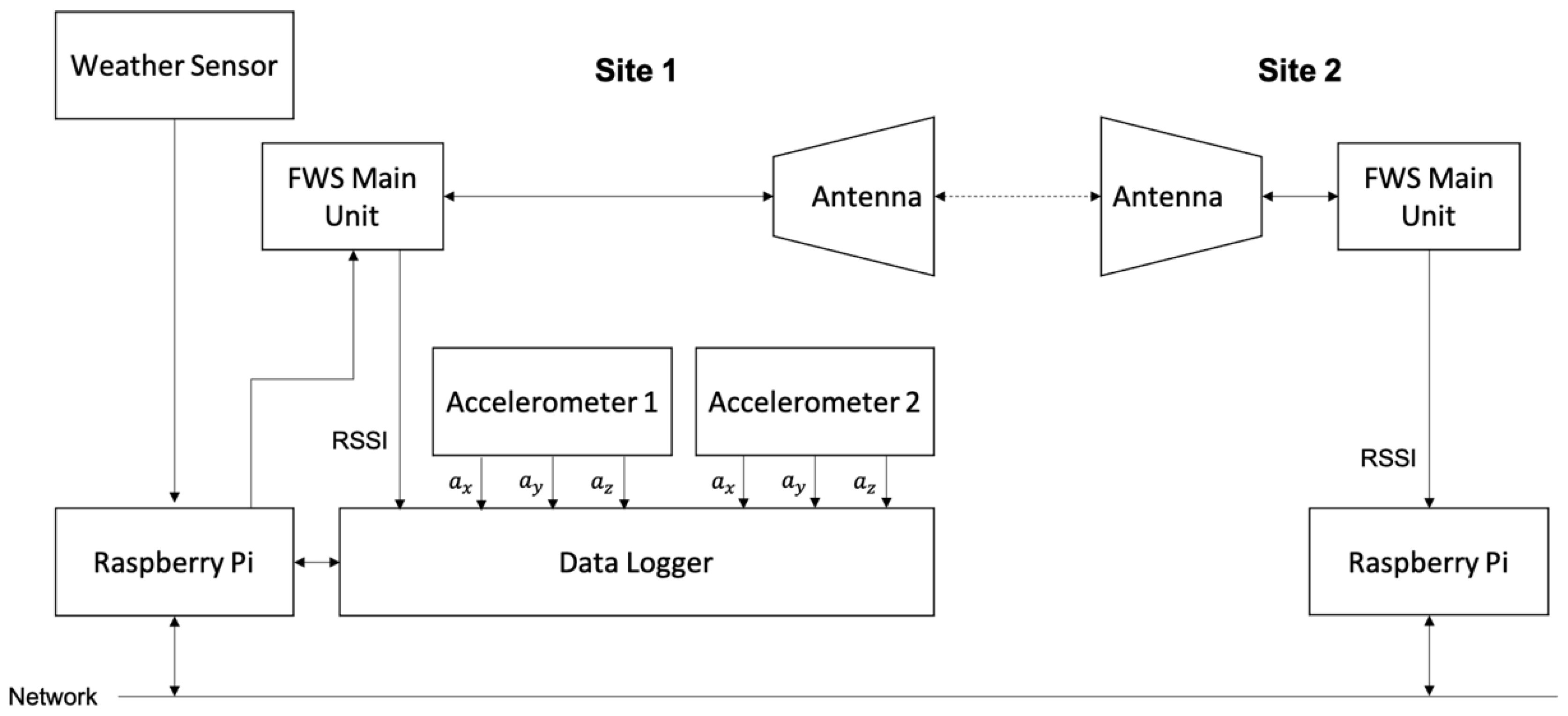
2. Experimental Setup
3. Theory and Algorithms
3.1. FWS Link Budget
3.2. Rain Attenuation
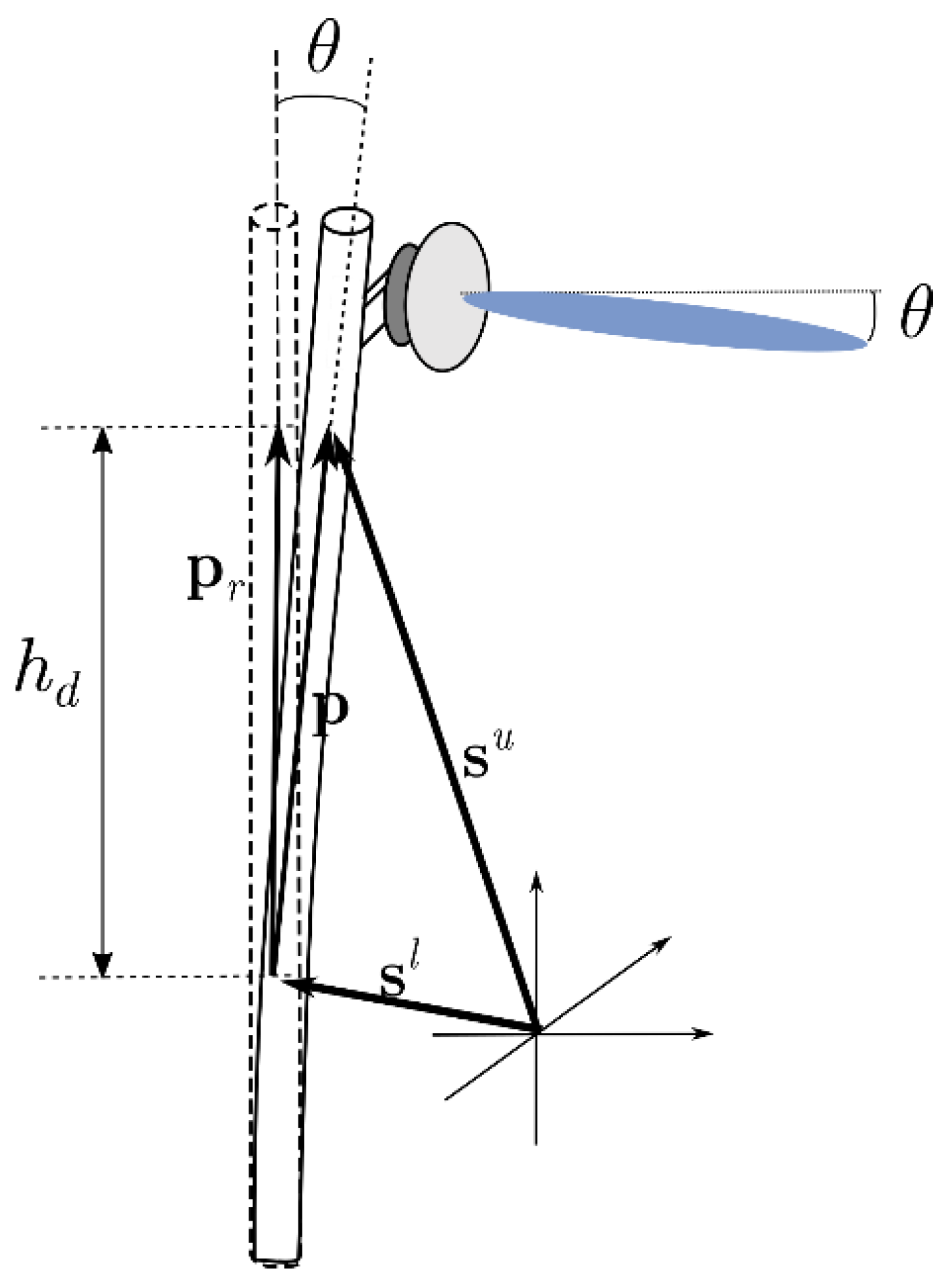
3.3. Inclination Attenuation Due to Wind
3.3.1. Dynamic Pole Angle Estimation via Wind-Induced Mechanical Vibration
3.3.2. Direct Dynamic Pole Angle Measurements via Accelerometer
4. Results and Analysis
4.1. The Distribution of Rain Rate and Wind Speed
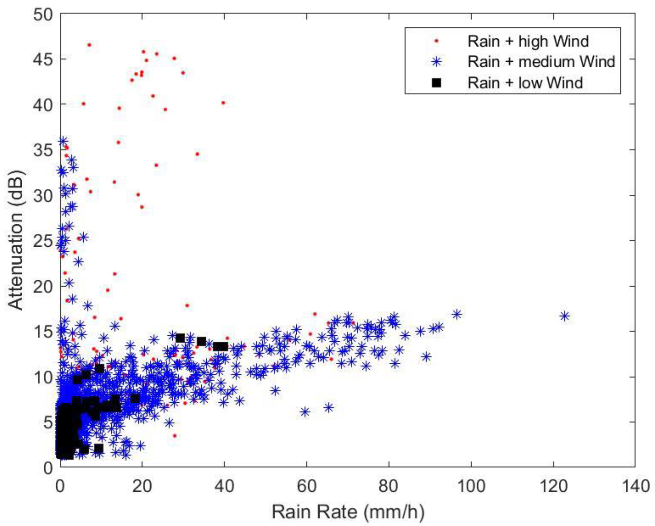
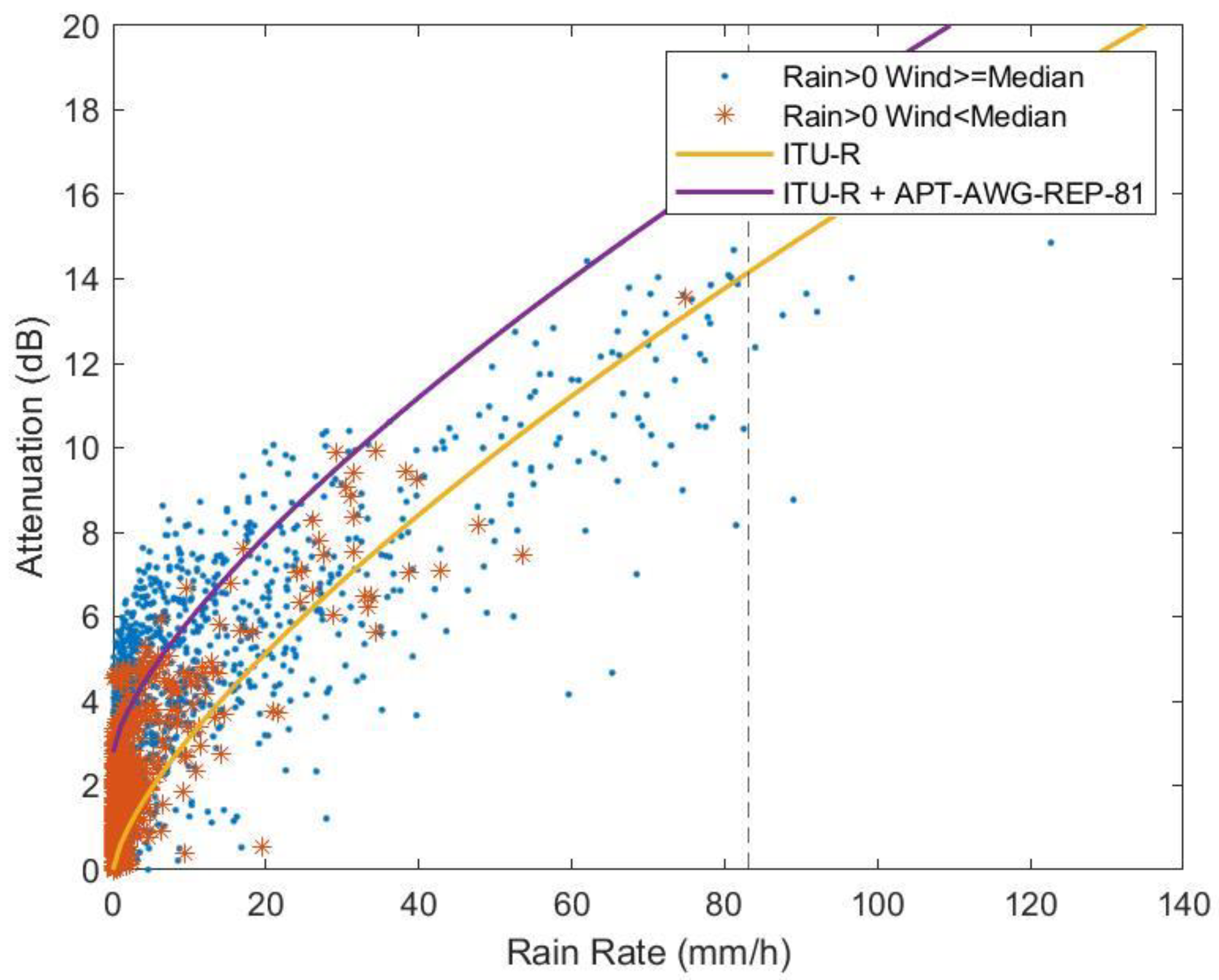
4.2. Rain Attenuation and Combined Rain-Wind Attenuation
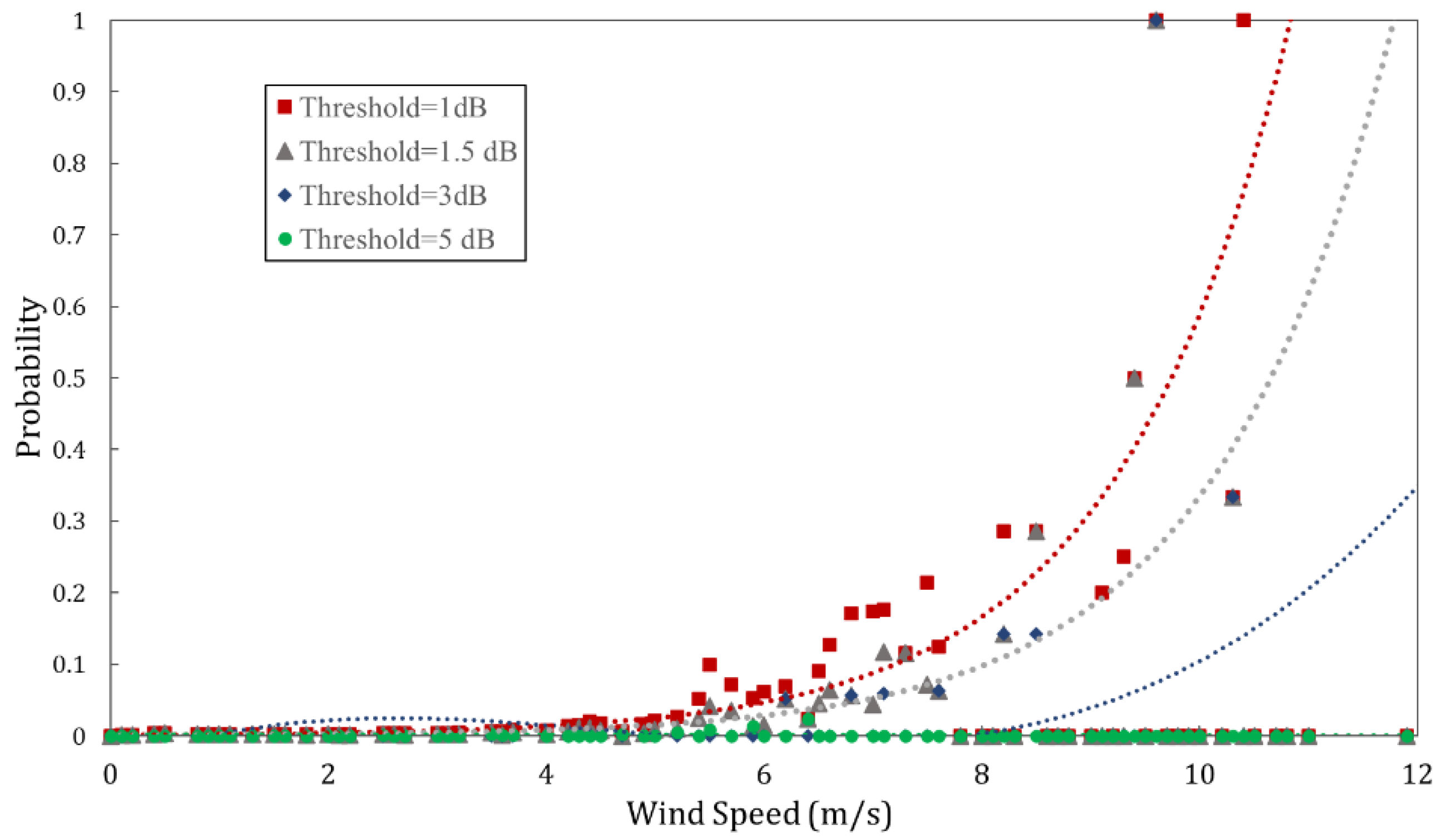
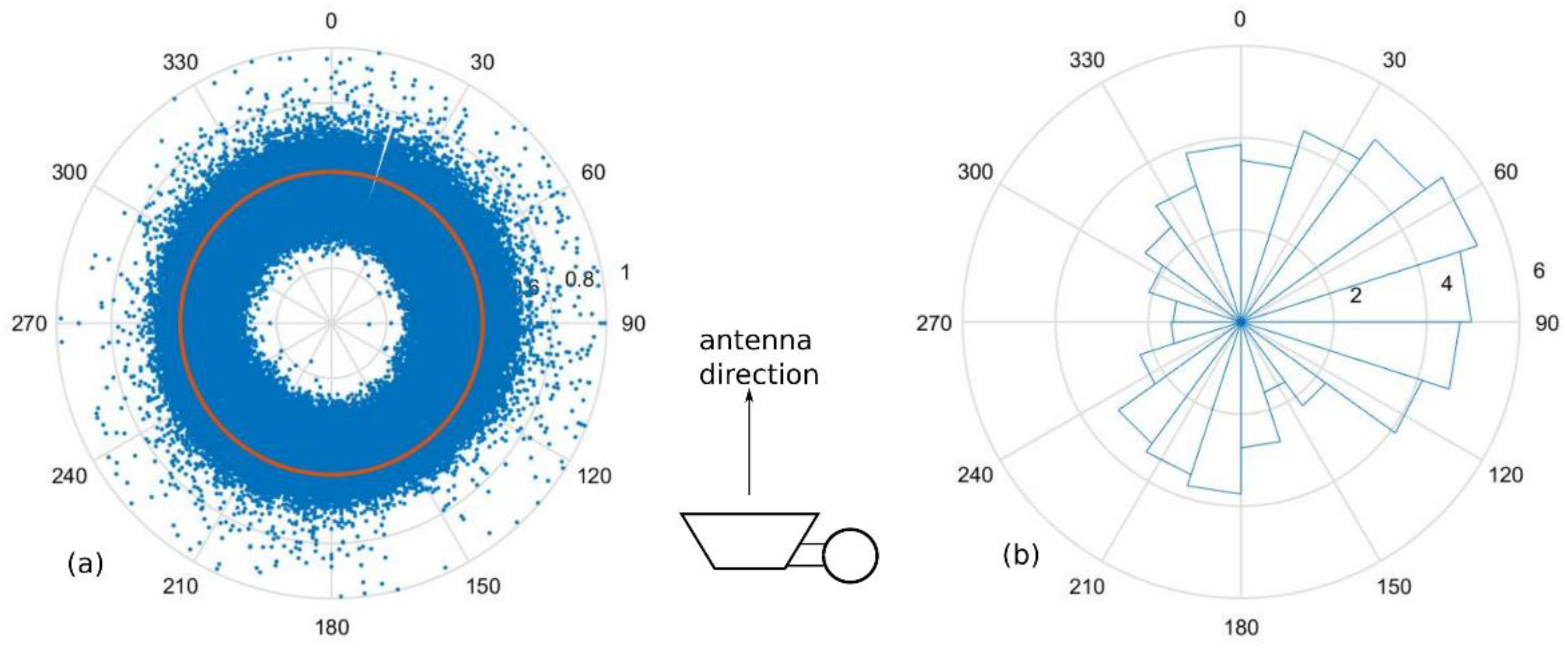
4.3. Wind-Induced Attenuation Using Direct Inclination Angle Measurement
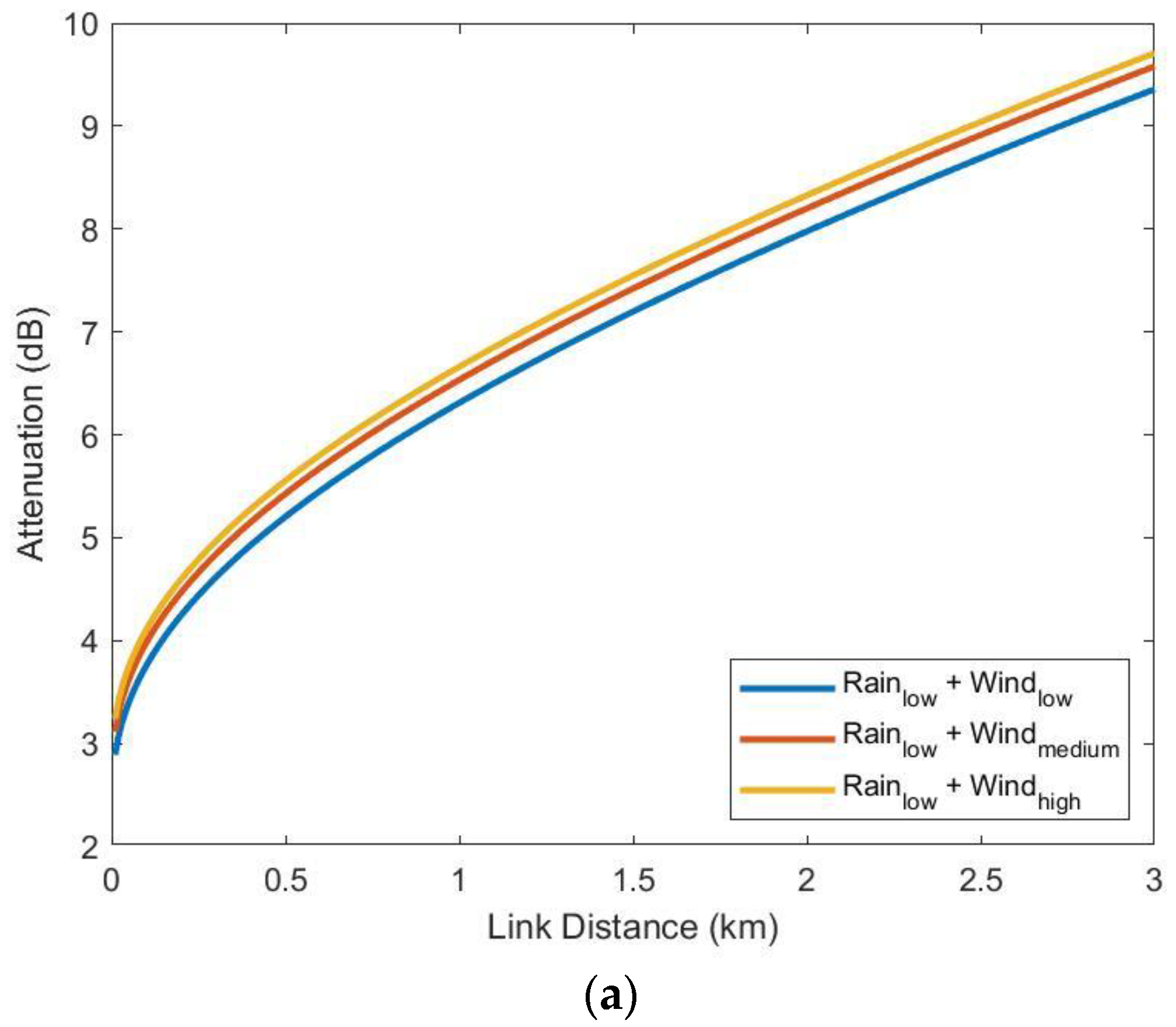
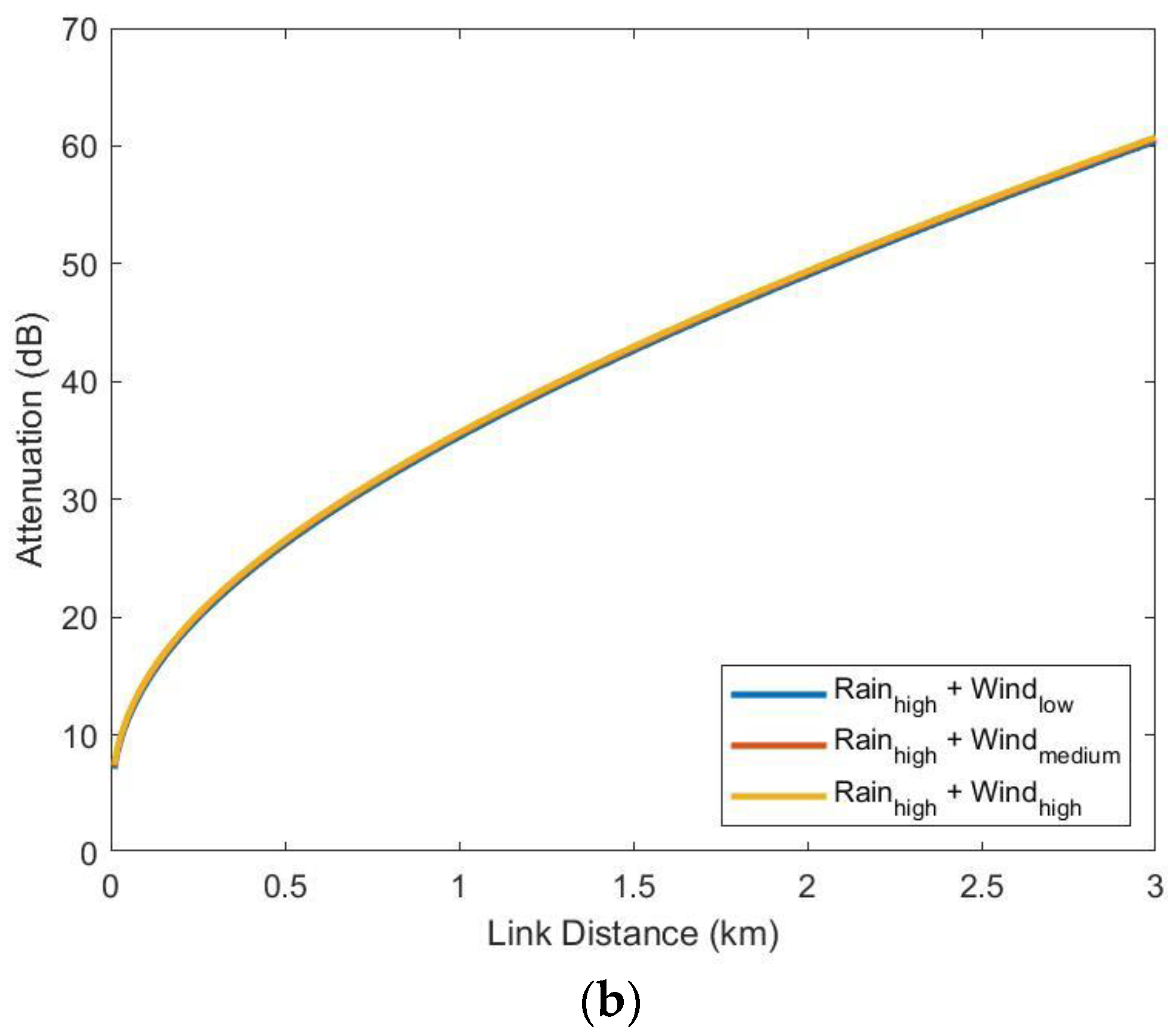
4.4. Dependence on the Polarization and the Link Distance
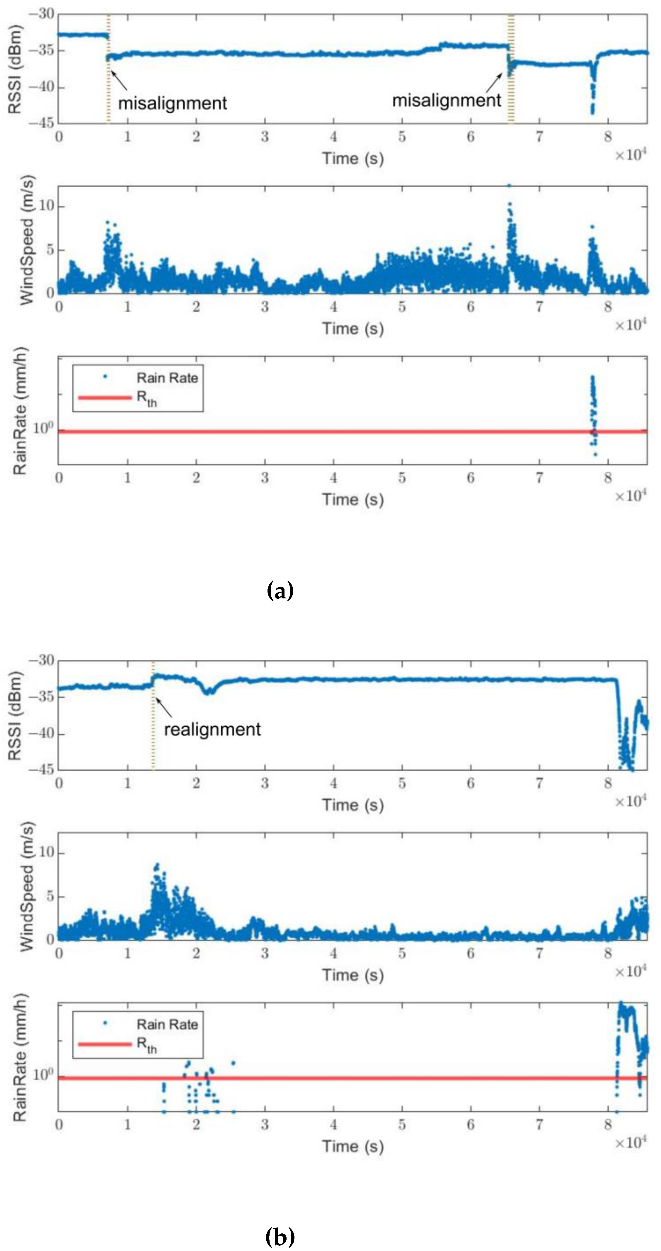
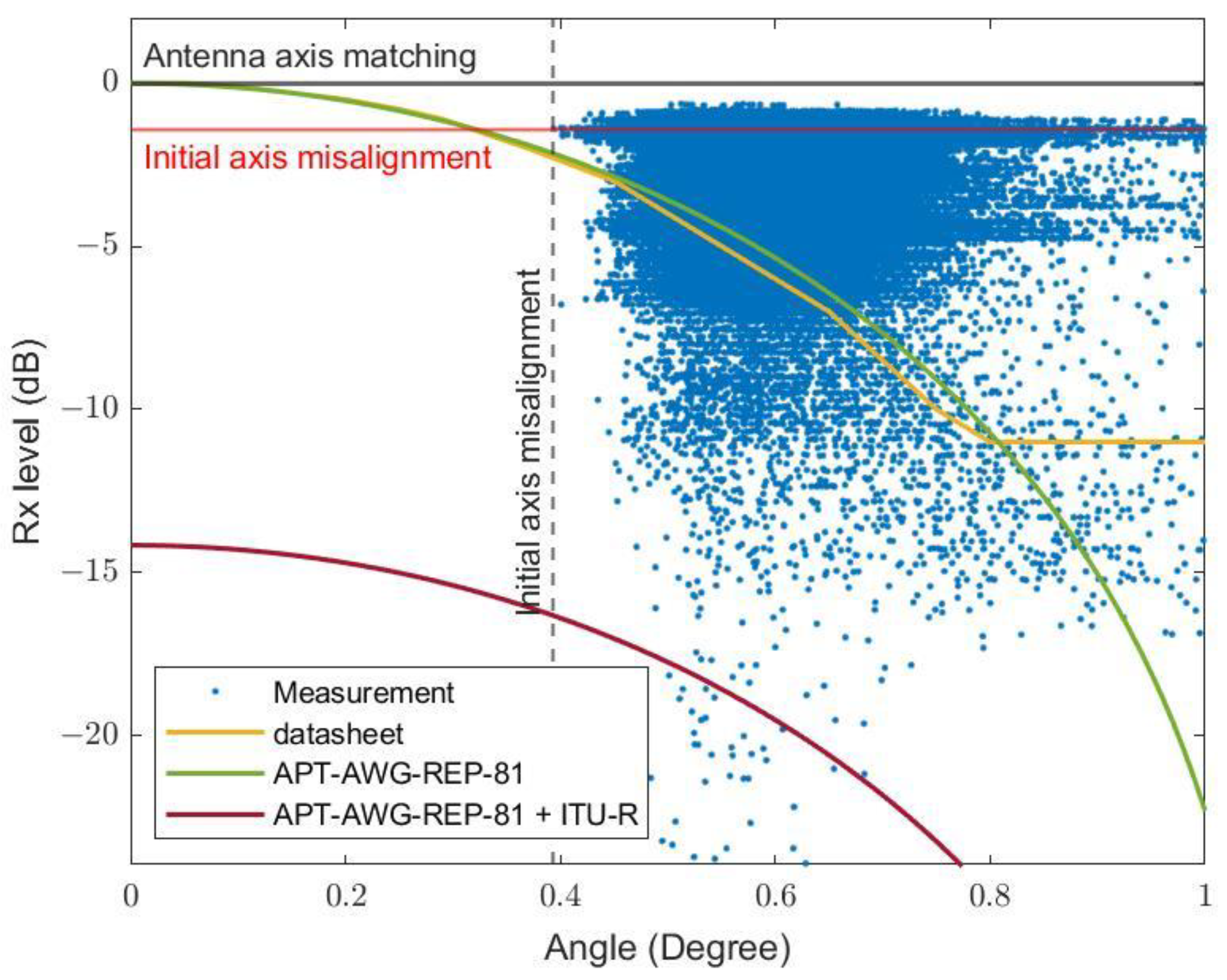
4.5. Antenna Misalignment and Realignment Due to Gust Events
5. Conclusions
Supplementary Materials
Author Contributions
Funding
Institutional Review Board Statement
Informed Consent Statement
Data Availability Statement
Acknowledgments
Conflicts of Interest
References
- Rappaport, T.S.; Xing, Y.; Kanhere, O.; Ju, S.; Madanayake, A.; Mandal, S.; Alkhateeb, A.; Trichopoulos, G.C. Wireless Communications and Applications Above 100 GHz: Opportunities and Challenges for 6G and Beyond. IEEE Access 2019, 7, 78729–78757. [Google Scholar] [CrossRef]
- Aldubaikhy, K.; Wu, W.; Zhang, N.; Cheng, N.; Shen, X. mmWave IEEE 802.11ay for 5G Fixed Wireless Access. IEEE Wirel. Commun. 2020, 27, 88–95. [Google Scholar] [CrossRef]
- Jung, B.K.; Dreyer, N.; Eckhard, J.M.; Kürner, T. Simulation and Automatic Planning of 300 GHz Backhaul Links. In Proceedings of the 2019 44th International Conference on Infrared, Millimeter, and Terahertz Waves (IRMMW-THz), Paris, France, 1–6 September 2019; pp. 1–3. [Google Scholar]
- Okumura, R.; Hirata, A. Automatic Planning of 300-GHz-Band Wireless Backhaul Link Deployment in Metropolitan Area. In Proceedings of the 2020 International Symposium on Antennas and Propagation (ISAP), Osaka, Japan, 25–28 January 2021; pp. 541–542. [Google Scholar]
- Jung, B.K.; Kürner, T. Automatic Planning Algorithm of 300 GHz Backhaul Links Using Ring Topology. In Proceedings of the 2021 15th European Conference on Antennas and Propagation (EuCAP), Düsseldorf, Germany, 22–26 March 2021; pp. 1–5. [Google Scholar]
- APT-AWG-REP-81, APT Report on FWS Link Performance under Severe Weather Conditions. Available online: https://www.apt.int/AWG-REPTS (accessed on 15 November 2022).
- Han, C.; Bi, Y.; Duan, S.; Lu, G. Rain Rate Retrieval Test from 25-GHz, 28-GHz, and 38-GHz Millimeter-Wave Link Measurement in Beijing. IEEE J. Sel. Top. Appl. Earth Obs. Remote Sens. 2019, 12, 2835–2847. [Google Scholar] [CrossRef]
- Messer, H.; Zinevich, A.; Alpert, P. Environmental sensor networks using existing wireless communication systems for rainfall and wind velocity measurements. IEEE Instrum. Meas. Mag. 2012, 15, 32–38. [Google Scholar] [CrossRef]
- Zheng, S.; Han, C.; Huo, J.; Cai, W.; Zhang, Y.; Li, P.; Zhang, G.; Ji, B.; Zhou, J. Research on Rainfall Monitoring Based on E-Band Millimeter Wave Link in East China. Sensors 2021, 21, 1670. [Google Scholar] [CrossRef] [PubMed]
- Lian, B.; Wei, Z.; Sun, X.; Li, Z.; Zhao, J. A Review on Rainfall Measurement Based on Commercial Microwave Links in Wireless Cellular Networks. Sensors 2022, 22, 4395. [Google Scholar] [CrossRef]
- Jin, W.; Kim, H.; Lee, H. A Novel Machine Learning Scheme for mmWave Path Loss Modeling for 5G Communications in Dense Urban Scenarios. Electronics 2022, 11, 1809. [Google Scholar] [CrossRef]
- Mao, K.; Zhu, Q.; Song, M.; Li, H.; Ning, B.; Pedersen, G.F.; Fan, W. Machine-Learning-Based 3-D Channel Modeling for U2V mmWave Communications. IEEE Internet Things J. 2022, 9, 17592–17607. [Google Scholar] [CrossRef]
- ITU-R. P.838-3; Specific Attenuation Model for Rain for Use in Prediction Methods. ITU-R: Geneva, Switzerland, 2005.
- ITU-R. P.530-18; Propagation Data and Prediction Methods Required for the Design of Terrestrial Line-of-Sight Systems. ITU-R: Geneva, Switzerland, 2021.
- Pontes, M.S.; Mello, L.D.S.; Souza, R.S.L.D.; Miranda, E.C.B. Review of Rain Attenuation Studies in Tropical and Equatorial Regions in Brazil. In Proceedings of the 2005 5th International Conference on Information Communications & Signal Processing, Bangkok, Thailand, 6–9 December 2005; pp. 1097–1101. [Google Scholar]
- Ulaganathen, K.; Rahman, T.A.; Rahim, S.K.A.; Islam, R.M. Review of Rain Attenuation Studies in Tropical and Equatorial Regions in Malaysia: An Overview. IEEE Antennas Propag. Mag. 2013, 55, 103–113. [Google Scholar] [CrossRef]
- Semire, F.A.; Mohd-Mokhtar, R.; Akanbi, I.A. Validation of New ITU-R Rain Attenuation Prediction Model over Malaysia Equatorial Region. MAPAN 2019, 34, 71–77. [Google Scholar] [CrossRef]
- Shayea, I.; Rahman, T.A.; Azmi, M.H.; Islam, M.R. Real Measurement Study for Rain Rate and Rain Attenuation Conducted Over 26 GHz Microwave 5G Link System in Malaysia. IEEE Access 2018, 6, 19044–19064. [Google Scholar] [CrossRef]
- Al-Saman, A.M.; Cheffena, M.; Mohamed, M.; Azmi, M.H.; Ai, Y. Statistical Analysis of Rain at Millimeter Waves in Tropical Area. IEEE Access 2020, 8, 51044–51061. [Google Scholar] [CrossRef]
- Al-Saman, A.; Mohamed, M.; Cheffena, M.; Azmi, M.H.; Rahman, T.A. Performance of Full-Duplex Wireless Back-Haul Link under Rain Effects Using E-Band 73 GHz and 83 GHz in Tropical Area. Appl. Sci. 2020, 10, 6138. [Google Scholar] [CrossRef]
- Al-Samman, A.M.; Mohamed, M.; Ai, Y.; Cheffena, M.; Azmi, M.H.; Rahman, T.A. Rain Attenuation Measurements and Analysis at 73 GHz E-Band Link in Tropical Region. IEEE Commun. Lett. 2020, 24, 1368–1372. [Google Scholar] [CrossRef]
- Zahid, O.; Salous, S. Long-Term Rain Attenuation Measurement for Short-Range mmWave Fixed Link Using DSD and ITU-R Prediction Models. Radio Sci. 2022, 57, e2021RS007307. [Google Scholar] [CrossRef]
- Huang, J.; Cao, Y.; Raimundo, X.; Cheema, A.; Salous, S. Rain Statistics Investigation and Rain Attenuation Modeling for Millimeter Wave Short-Range Fixed Links. IEEE Access 2019, 7, 156110–156120. [Google Scholar] [CrossRef]
- Hirata, A.; Yamaguchi, R.; Takahashi, H.; Kosugi, T.; Murata, K.; Kukutsu, N.; Kado, Y. Effect of Rain Attenuation for a 10-Gb/s 120-GHz-Band Millimeter-Wave Wireless Link. IEEE Trans. Microw. Theory Tech. 2009, 57, 3099–3105. [Google Scholar] [CrossRef]
- Norouzian, F.; Marchetti, E.; Gashinova, M.; Hoare, E.; Constantinou, C.; Gardner, P.; Cherniakov, M. Rain Attenuation at Millimeter Wave and Low-THz Frequencies. IEEE Trans. Antennas Propag. 2020, 68, 421–431. [Google Scholar] [CrossRef]
- Jung, B.K.; Kürner, T. Performance analysis of 300 GHz backhaul links using historic weather data. Adv. Radio Sci. 2021, 19, 153–163. [Google Scholar] [CrossRef]
- Weng, Z.K.; Kanno, A.; Dat, P.T.; Inagaki, K.; Tanabe, K.; Sasaki, E.; Kürner, T.; Jung, B.K.; Kawanishi, T. Millimeter-Wave and Terahertz Fixed Wireless Link Budget Evaluation for Extreme Weather Conditions. IEEE Access 2021, 9, 163476–163491. [Google Scholar] [CrossRef]
- Available online: https://www.commscope.com/globalassets/digizuite/46906-7287a-3-29-19-pdf.pdf (accessed on 12 November 2022).
- ITU-R. P.676-13; Attenuation by Atmospheric Gases and Related Effects. ITU-R: Geneva, Switzerland, 2022.
- ITU-R. P.835-6; Reference Standard Atmospheres. ITU-R: Geneva, Switzerland, 2017.
- ITU-R. P.837-6; Characteristics of Precipitation for Propagation Modelling. ITU-R: Geneva, Switzerland, 2017.
- Budalal, A.A.H.; Islam, M.R.; Abdullah, K.; Rahman, T.A. Modification of Distance Factor in Rain Attenuation Prediction for Short-Range Millimeter-Wave Links. IEEE Antennas Wirel. Propag. Lett. 2020, 19, 1027–1031. [Google Scholar] [CrossRef]
- Manabe, T.; Ihara, T.; Furuhama, Y. Inference of raindrop size distribution from attenuation and rain rate measurements. IEEE Trans. Antennas Propag. 1984, 32, 474–478. [Google Scholar] [CrossRef]
- Heddleson, C.F.; Brown, D.L.; Cliffe, R.T. Summary of Drag Coefficients of Various Shaped Cylinders; General Electric: Cincinnati, OH, USA, 1957. [Google Scholar]
- Beer, F.P.; Johnston, E.R.; Mazurek, D.F.; Cornwell, P.J.; Self, B.P. Vector Mechanics for Engineers: Statics and Dynamics; McGraw-Hill Education: New York, NY, USA, 2018. [Google Scholar]


| Parameters | Values | Calculation Method/Reference |
|---|---|---|
| −5 dBm | User setting | |
| 43 dB | Datasheet | |
| Free-space loss () | 113.4 dB | at f = 74.625 GHz and r0 = 150 m |
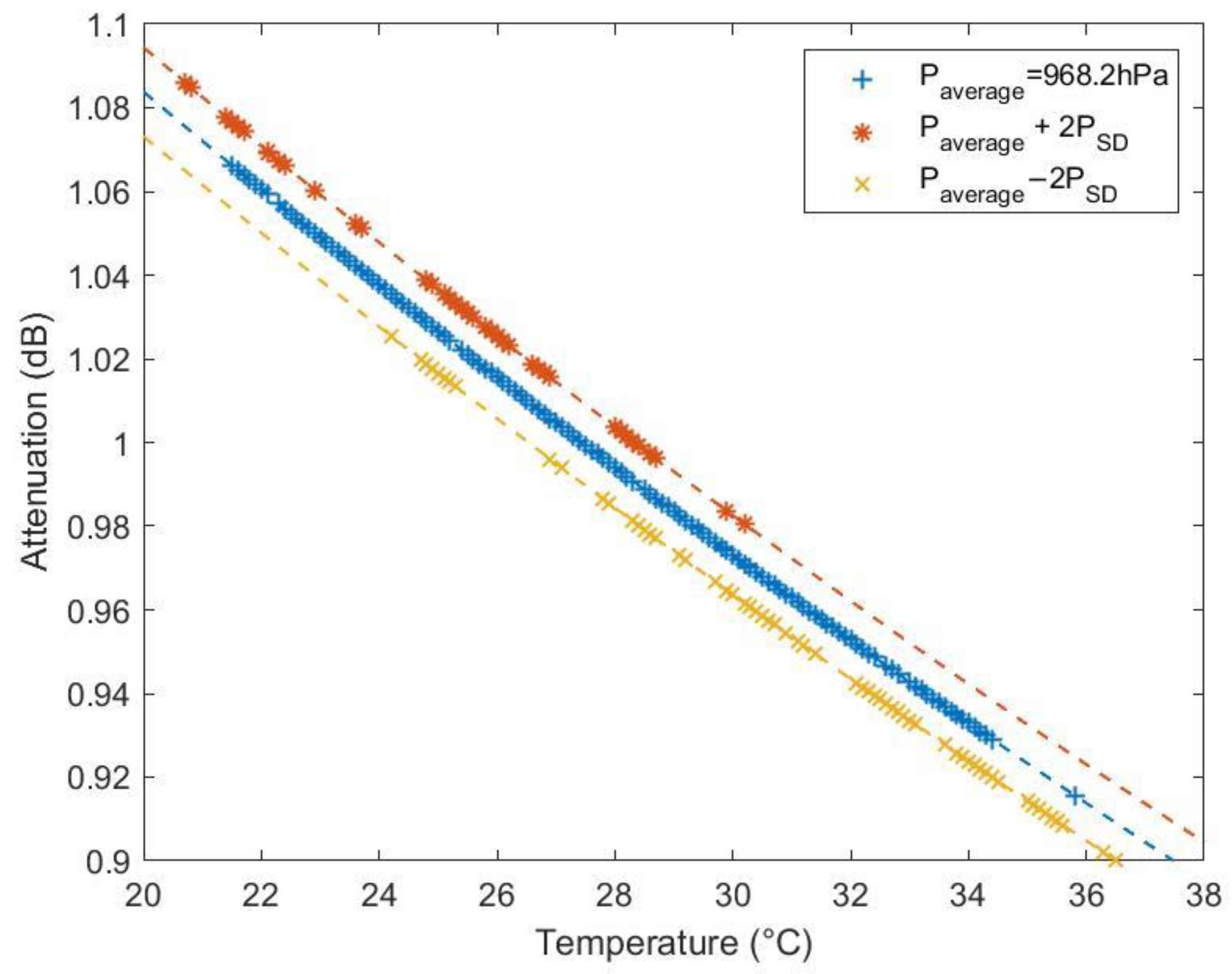
| 0.899–1.087 dB | ITU-R P.676 [29] |
| Symbol | Quantity | Value | Unit |
|---|---|---|---|
| Drag coefficient of the pole | 0.98 | - | |
| Wind receiving area of the pole | 0.36 | m2 | |
| Drag coefficient of the antenna | 1.42 | - | |
| Wind receiving area of the antenna | 0.118 | m2 | |
| Air density | 1.124 | kg/m3 | |
| Pole length | 4 | m | |
| Pole diameter | 101.6 (4) | mm (inch) | |
| Antenna diameter | 0.3 (1) | m (ft) | |
| Young’s modulus | 200 × 109 | Pa | |
| Second moment of area | 1.8 × 10⁻⁶ | m4 |
Disclaimer/Publisher’s Note: The statements, opinions and data contained in all publications are solely those of the individual author(s) and contributor(s) and not of MDPI and/or the editor(s). MDPI and/or the editor(s) disclaim responsibility for any injury to people or property resulting from any ideas, methods, instructions or products referred to in the content. |
© 2023 by the authors. Licensee MDPI, Basel, Switzerland. This article is an open access article distributed under the terms and conditions of the Creative Commons Attribution (CC BY) license (https://creativecommons.org/licenses/by/4.0/).
Share and Cite
Mankong, U.; Chamsuk, P.; Nakprasert, S.; Potha, S.; Weng, Z.-K.; Dat, P.T.; Kanno, A.; Kawanishi, T. Millimeter Wave Attenuation Due to Wind and Heavy Rain in a Tropical Region. Sensors 2023, 23, 2532. https://doi.org/10.3390/s23052532
Mankong U, Chamsuk P, Nakprasert S, Potha S, Weng Z-K, Dat PT, Kanno A, Kawanishi T. Millimeter Wave Attenuation Due to Wind and Heavy Rain in a Tropical Region. Sensors. 2023; 23(5):2532. https://doi.org/10.3390/s23052532
Chicago/Turabian StyleMankong, Ukrit, Pakawat Chamsuk, Sitthichok Nakprasert, Sangdaun Potha, Zu-Kai Weng, Pham Tien Dat, Atsushi Kanno, and Tetsuya Kawanishi. 2023. "Millimeter Wave Attenuation Due to Wind and Heavy Rain in a Tropical Region" Sensors 23, no. 5: 2532. https://doi.org/10.3390/s23052532
APA StyleMankong, U., Chamsuk, P., Nakprasert, S., Potha, S., Weng, Z.-K., Dat, P. T., Kanno, A., & Kawanishi, T. (2023). Millimeter Wave Attenuation Due to Wind and Heavy Rain in a Tropical Region. Sensors, 23(5), 2532. https://doi.org/10.3390/s23052532