Author Contributions
Conceptualization, T.H., H.K. and K.K.; methodology, T.H.; software, T.H.; writing—original draft preparation, T.H.; writing—review and editing, H.K. and K.K.; supervision, K.K.; project administration, K.K.; funding acquisition, K.K. All authors have read and agreed to the final version of the manuscript.
Figure 1.
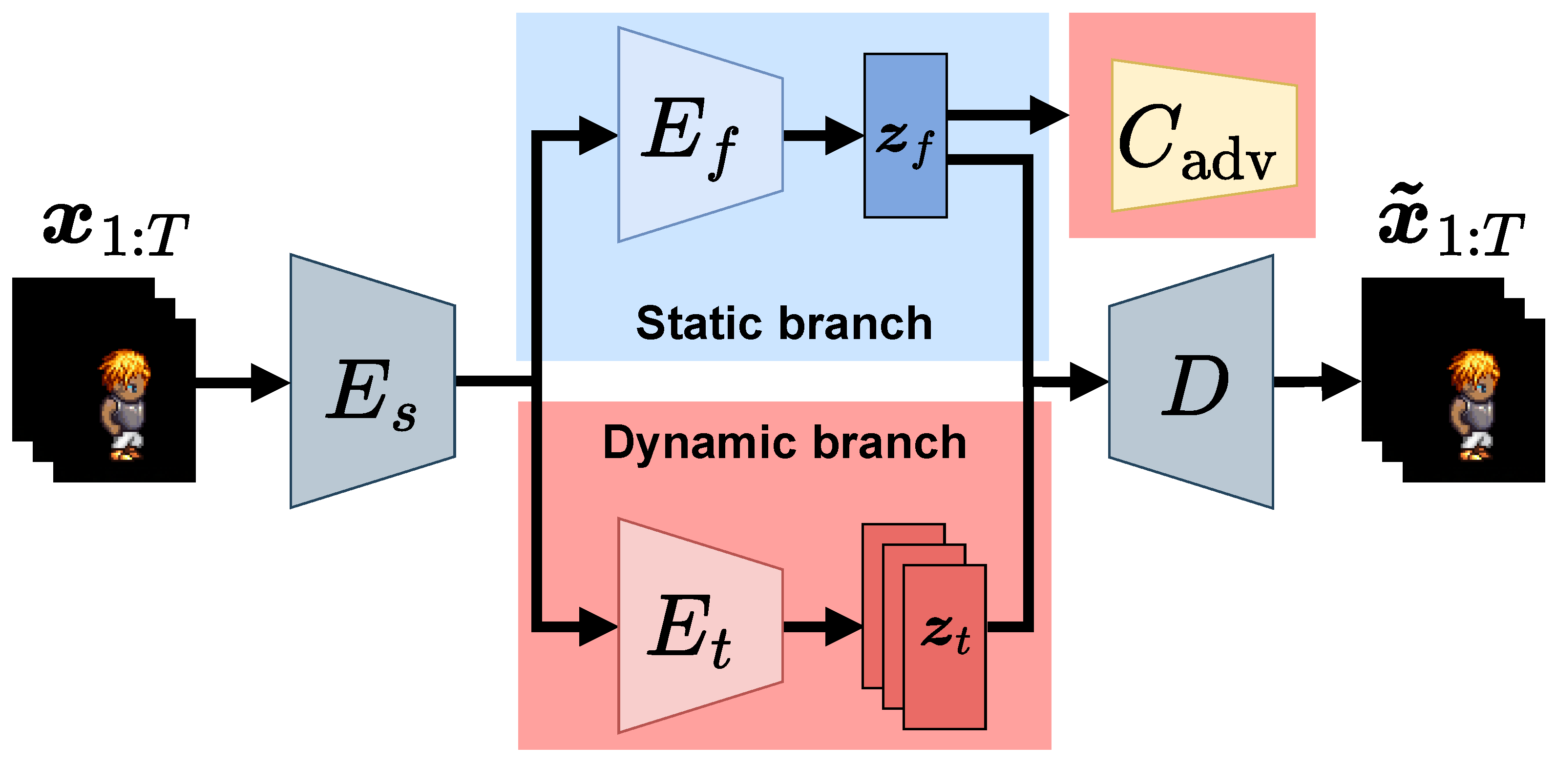
Overview of proposed model. The model consists of an auxiliary adversarial classifier , a decoder D, a shared encoder , a static encoder , and a dynamic encoder . and denote input and reconstructed videos, respectively, and and indicate static and dynamic latent variables, respectively.
Figure 1.
Overview of proposed model. The model consists of an auxiliary adversarial classifier , a decoder D, a shared encoder , a static encoder , and a dynamic encoder . and denote input and reconstructed videos, respectively, and and indicate static and dynamic latent variables, respectively.
Figure 4.
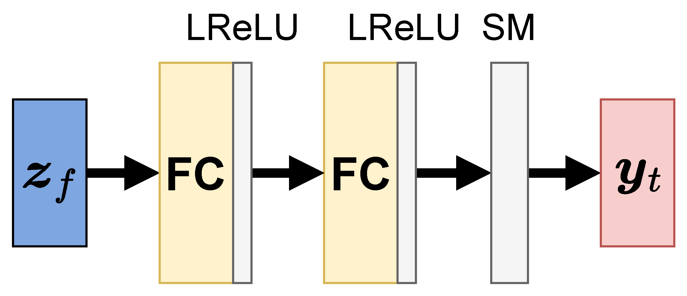
Overview of the auxiliary adversarial classifier . The classifier consists of MLP with two fully connected (FC) layers and leaky ReLU (LReLU) and a softmax (SM) layer. The output is the predicted distribution of class labels for dynamic features.
Figure 4.
Overview of the auxiliary adversarial classifier . The classifier consists of MLP with two fully connected (FC) layers and leaky ReLU (LReLU) and a softmax (SM) layer. The output is the predicted distribution of class labels for dynamic features.
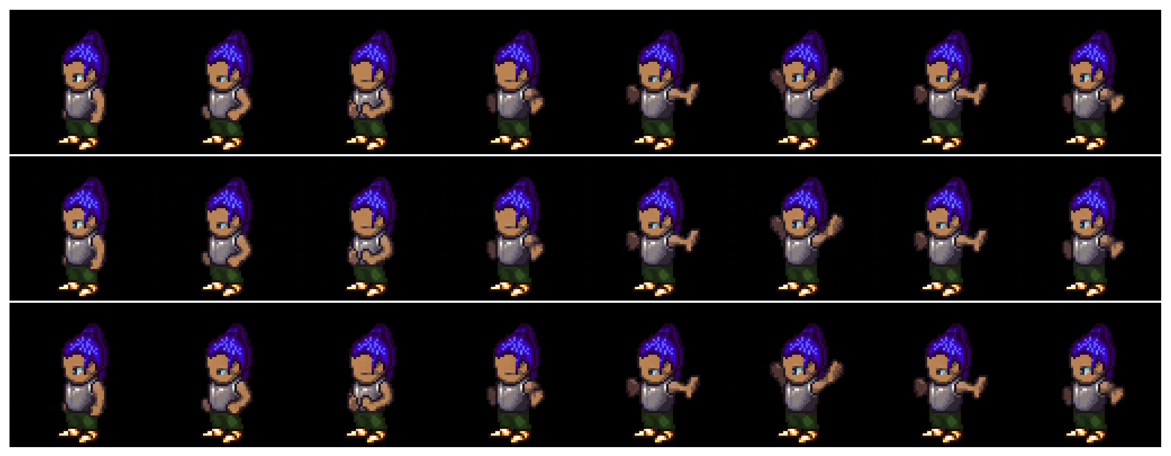
Figure 5.
Example of reconstruction on the Sprites dataset. The top, middle, and bottom rows denote the input video and results using the DSVAE and proposed methods, respectively.
Figure 5.
Example of reconstruction on the Sprites dataset. The top, middle, and bottom rows denote the input video and results using the DSVAE and proposed methods, respectively.
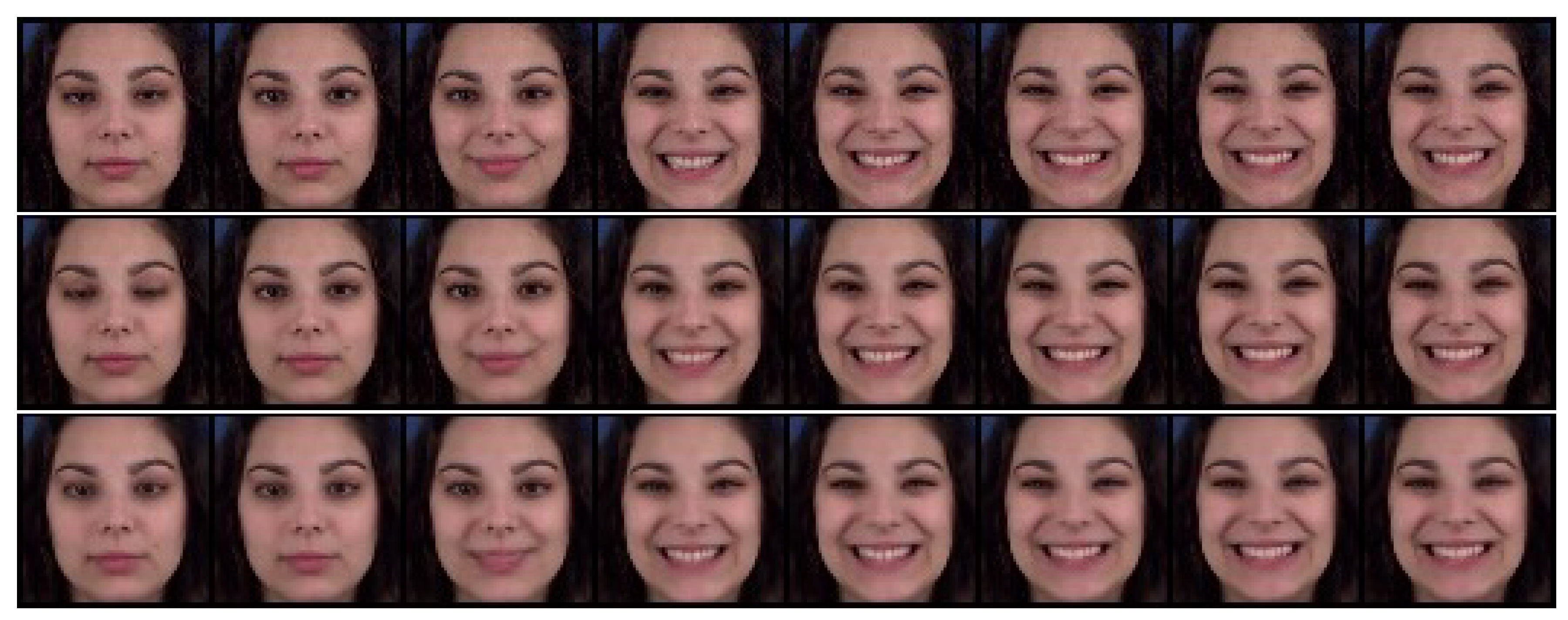
Figure 6.
Example of reconstruction on the MUG dataset. The top, middle, and bottom rows denote the input video and the results using DSVAE and the proposed method, respectively.
Figure 6.
Example of reconstruction on the MUG dataset. The top, middle, and bottom rows denote the input video and the results using DSVAE and the proposed method, respectively.
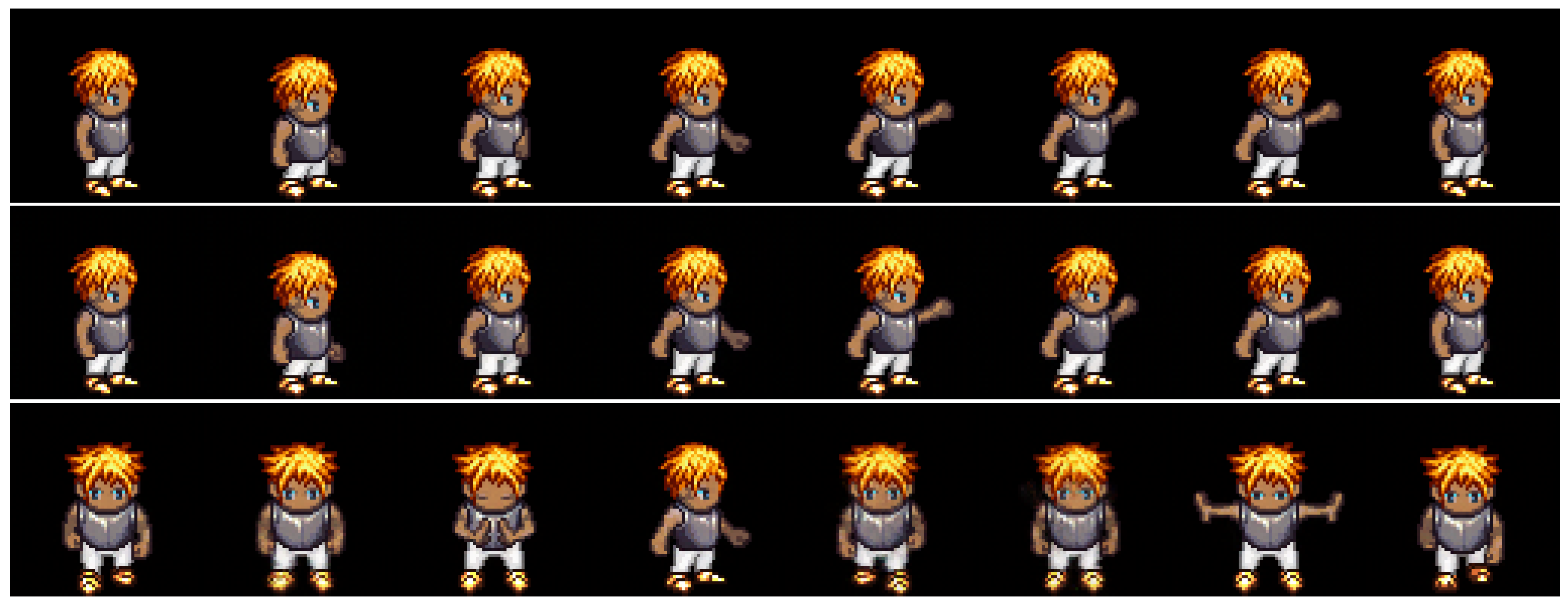
Figure 7.
Example of zero-replaced generation on the Sprites dataset. We fixed the dynamic variables and replaced the static variable with zero. The top, middle, and bottom rows denote the input video and the results using DSVAE and the proposed method, respectively.
Figure 7.
Example of zero-replaced generation on the Sprites dataset. We fixed the dynamic variables and replaced the static variable with zero. The top, middle, and bottom rows denote the input video and the results using DSVAE and the proposed method, respectively.
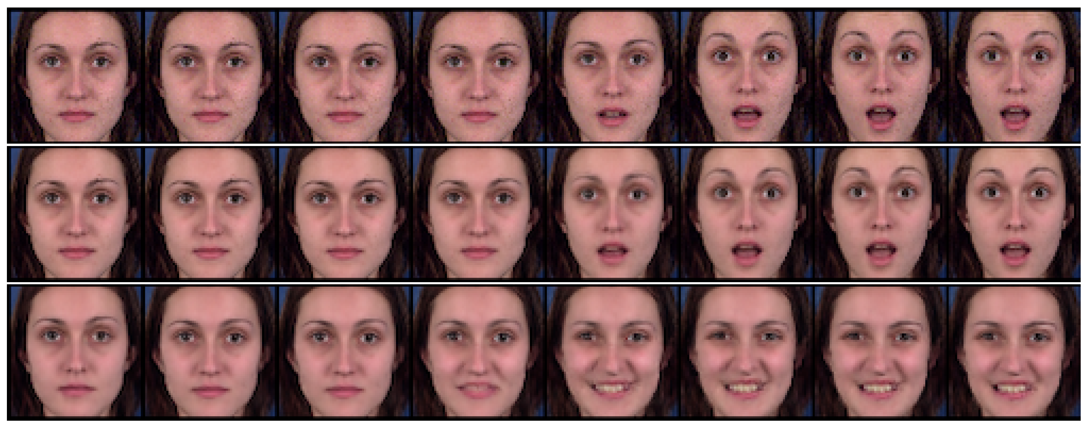
Figure 8.
Example of zero-replaced generation on the MUG dataset. We fixed the dynamic variables and replaced the static variable with zero. The top, middle, and bottom rows denote the input video and the results using DSVAE and the proposed method, respectively.
Figure 8.
Example of zero-replaced generation on the MUG dataset. We fixed the dynamic variables and replaced the static variable with zero. The top, middle, and bottom rows denote the input video and the results using DSVAE and the proposed method, respectively.
Figure 9.
Example of randomly sampled generation on the Sprites dataset. We fixed the static variable and randomly sampled the dynamic variables. The top, middle, and bottom rows denote the input video and the results using DSVAE and the proposed method, respectively.
Figure 9.
Example of randomly sampled generation on the Sprites dataset. We fixed the static variable and randomly sampled the dynamic variables. The top, middle, and bottom rows denote the input video and the results using DSVAE and the proposed method, respectively.
Figure 10.
Example of randomly sampled generation on the MUG dataset. We fixed the static variable and randomly sampled the dynamic variables. The top, middle, and bottom rows denote the input video and the results using DSVAE and the proposed method, respectively.
Figure 10.
Example of randomly sampled generation on the MUG dataset. We fixed the static variable and randomly sampled the dynamic variables. The top, middle, and bottom rows denote the input video and the results using DSVAE and the proposed method, respectively.
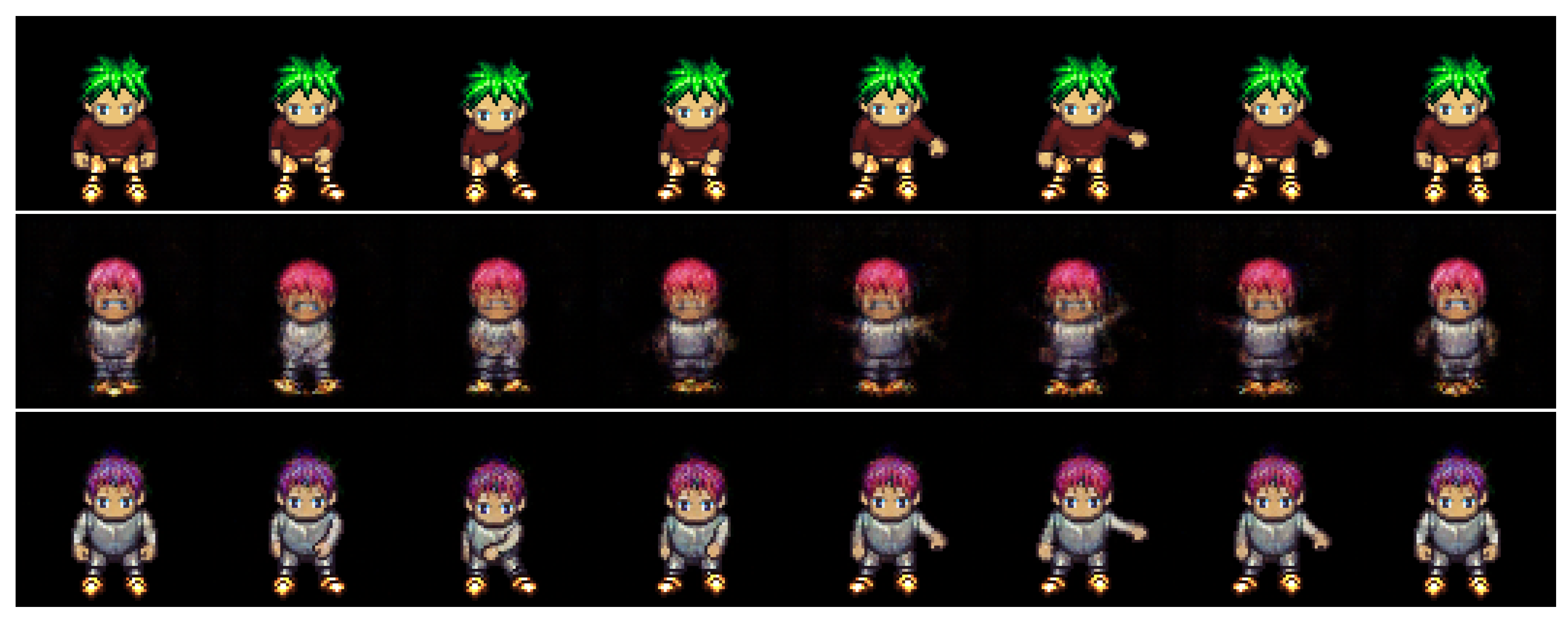
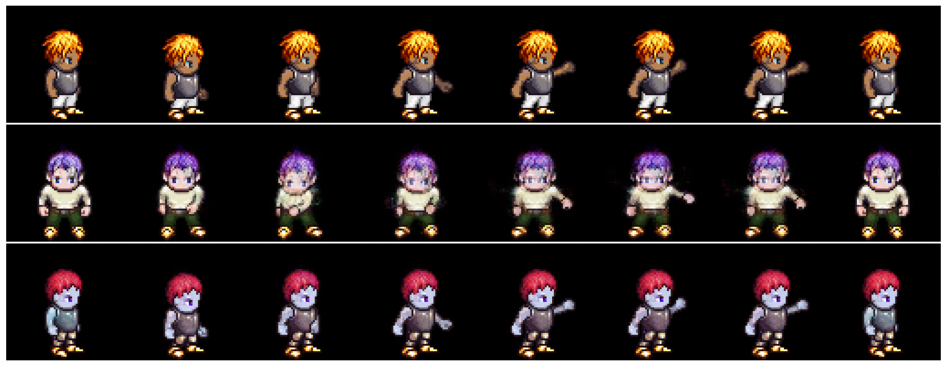
Figure 11.
Example of randomly sampled generation on the Sprites dataset. We fixed the dynamic variables and randomly sampled the static variable. The top, middle, and bottom rows denote the input video and the results using DSVAE and the proposed method, respectively.
Figure 11.
Example of randomly sampled generation on the Sprites dataset. We fixed the dynamic variables and randomly sampled the static variable. The top, middle, and bottom rows denote the input video and the results using DSVAE and the proposed method, respectively.
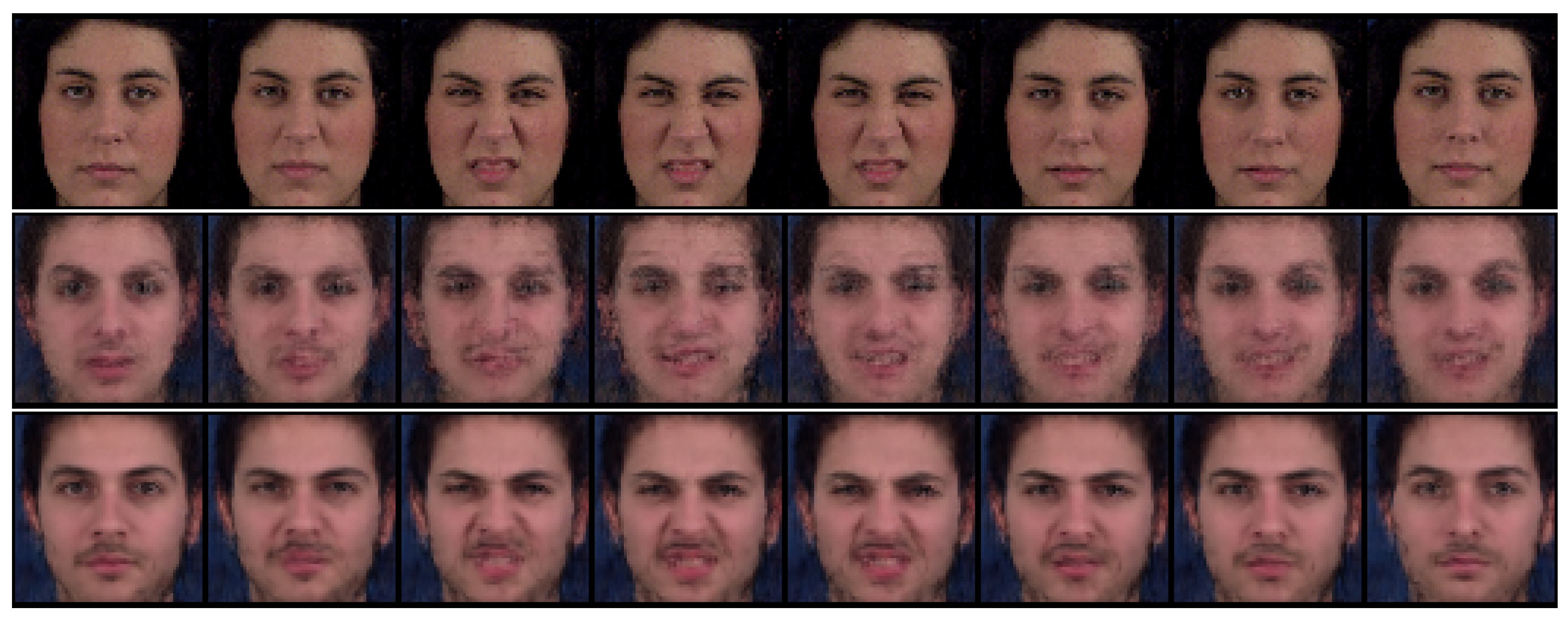
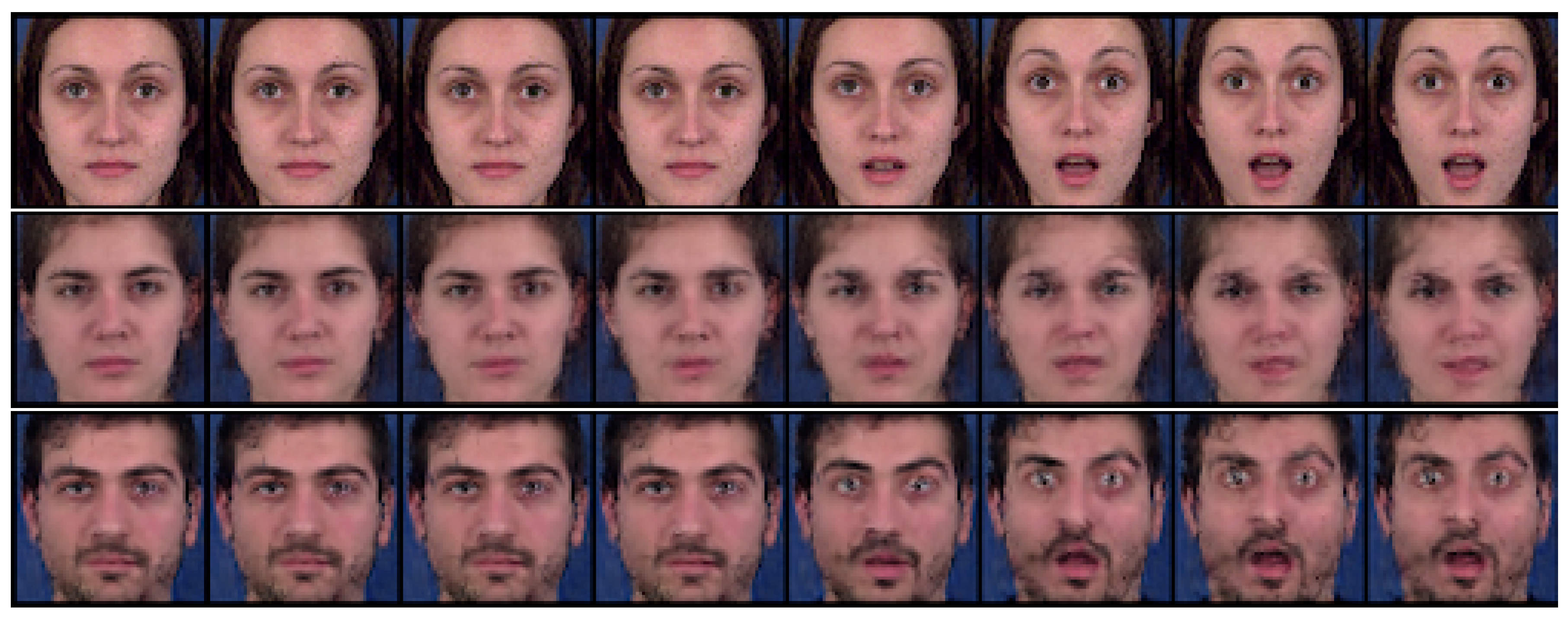
Figure 12.
Example of randomly sampled generation on the MUG dataset. We fixed the dynamic variables and randomly sampled the static variable. The top, middle, and bottom rows denote the input video and the results using DSVAE and the proposed method, respectively.
Figure 12.
Example of randomly sampled generation on the MUG dataset. We fixed the dynamic variables and randomly sampled the static variable. The top, middle, and bottom rows denote the input video and the results using DSVAE and the proposed method, respectively.
Table 1.
Learning condition for the Sprites dataset.
Table 1.
Learning condition for the Sprites dataset.
| Appearance | 1296 (4 parts × 6 categories) |
| | (train = 1000, test = 296) |
| Motion | 9 () |
| Format | (channel, frame, height, weight) = (3, 8, 64, 64) |
| Batch size | 100 |
| Training Epochs | 1000 |
| Optimization | Adam (, , ) |
| Dimension | 32 |
| Dimension | 256 |
Table 2.
Learning condition for the MUG dataset.
Table 2.
Learning condition for the MUG dataset.
| Subject | 52 (train:test = 3:1) |
| Expression | 6 |
| Format | (channel, frame, height, weight) = (3, 8, 64, 64) |
| Batch size | 128 |
| Training Epochs | 5000 |
| Optimization | Adam (, , ) |
| Dimension of | 128 |
| Dimension of | 128 |
Table 3.
Root-mean-squared error for reconstruction task.
Table 3.
Root-mean-squared error for reconstruction task.
| (a) Sprites | |
| | RMSE |
| DSVAE [14] | |
| Ours | |
| (b) MUG | |
| | RMSE |
| DSVAE [14] | |
| Ours | |
Table 4.
Average classification accuracy over ten runs (%) for the fixed static latent variable and randomly sampled dynamic latent variables.
Table 4.
Average classification accuracy over ten runs (%) for the fixed static latent variable and randomly sampled dynamic latent variables.
| (a) Sprites | | |
| | Static | Dynamic |
| DSVAE [14] | 100.0 ± 0.0 | 100.0 ± 0.0 |
| Ours | 99.0 ± 0.2 | 11.3 ± 0.4 |
| Ground Truth | 100.0 | - |
| Random Accuracy | - | 11.1 |
| (b) MUG | | |
| | Static ↑ | Dynamic |
| DSVAE [14] | 100.0 ± 0.0 | 99.4 ± 0.1 |
| Ours | 99.9 ± 0.1 | 21.1 ± 1.0 |
| Ground Truth | 100.0 | - |
| Random Accuracy | - | 16.7 |
Table 5.
Classification accuracy (%) for the fixed dynamic latent variables and randomly sampled static latent variables. For C-DSVAE (reproduced) and ours, the average classification accuracy over ten runs is presented; the others are taken from the literature [
14,
15,
16,
17].
Table 5.
Classification accuracy (%) for the fixed dynamic latent variables and randomly sampled static latent variables. For C-DSVAE (reproduced) and ours, the average classification accuracy over ten runs is presented; the others are taken from the literature [
14,
15,
16,
17].
| (a) Sprites | | |
| | Static | Dynamic |
| DSVAE [14] | - | 90.73 |
| S3VAE [15] | - | 99.49 |
| R-WAE [16] | - | 98.98 |
| C-DSVAE [17] | - | 99.99 |
| C-DSVAE (reproduced) | 16.55 ± 0.36 | 100.0 ± 0.0 |
| Ours | 16.47 ± 0.13 | 100.0 ± 0.0 |
| Ground Truth | - | 100.0 |
| Random Accuracy | 16.67 | - |
| (b) MUG | | |
| | Static | Dynamic |
| DSVAE [14] | - | 54.29 |
| S3VAE [15] | - | 70.51 |
| R-WAE [16] | - | 71.25 |
| C-DSVAE [17] | - | 81.16 |
| C-DSVAE (reproduced) | 2.46 ± 0.34 | 47.03 ± 0.97 |
| Ours | 2.85 ± 0.69 | 77.52 ± 0.90 |
| Ground Truth | - | 100.0 |
| Random Accuracy | 1.92 | - |
Table 6.
Entropy-based metrics for the fixed dynamic latent variable and randomly sampled static latent variable. For C-DSVAE (reproduced) and our method, the average classification accuracies over ten runs are presented; the others are taken from the literature [
14,
15,
16,
17]. In the tables, the upward (downward) arrows ↑ (↓) indicate that the higher (lower) the values, the better.
| (a) Sprites | | | |
| | | | |
| DSVAE [14] | 8.384 | 0.072 | 2.192 |
| S3VAE [15] | 8.637 | 0.041 | 2.197 |
| R-WAE [16] | 8.516 | 0.055 | 2.197 |
| C-DSVAE [17] | 8.637 | 0.041 | 2.197 |
| C-DSVAE (reproduced) | 8.999 ± 0.000 | 0.0001 ± 0.0000 | 2.197 ± 0.000 |
| Ours | | | |
| Ground Truth | 9.0 | 0.0 | 2.197 |
| (b) MUG | | | |
| | | | |
| DSVAE [14] | 3.608 | 0.374 | 1.657 |
| S3VAE [15] | 5.136 | 0.135 | 1.760 |
| R-WAE [16] | 5.149 | 0.131 | 1.771 |
| C-DSVAE [17] | 5.341 | 0.092 | 1.775 |
| C-DSVAE (reproduced) | 2.362 ± 0.052 | 0.855 ± 0.019 | 1.714 ± 0.006 |
| Ours | | | |
| Ground Truth | 6.0 | 0.0 | 1.792 |


