Time Domain Transmissiometry-Based Sensor for Simultaneously Measuring Soil Water Content, Electrical Conductivity, Temperature, and Matric Potential

Abstract

Owing to the increasing popularity of smart agriculture in recent years, it is necessary to develop a single sensor that can measure several soil properties, particularly the soil water content and matric potential. Therefore, in this study, we developed a sensor that can simultaneously measure soil water content (θ), electrical conductivity (σ_b), temperature, and matric potential (ψ). The proposed sensor can determine θ and σ_b using time domain transmissiometry and can determine ψ based on the capacitance of the accompanying ceramic plate. A series of laboratory and field tests were conducted to evaluate the performance of the sensor. The sensor output values were correlated with the soil properties, and the temperature dependence of the sensor outputs was evaluated. Additionally, field tests were conducted to measure transient soil conditions over a long period. The results show that the developed sensor can measure each soil property with acceptable accuracy. Moreover, the root-mean-square errors of the sensor and reference values were 1.7 for the dielectric constant (which is equivalent to θ), 62 mS m⁻¹ for σ_b, and 0.05–0.88 for log ψ. The temperature dependence was not a problem, except when ψ was below −100 kPa. The sensor can be used for long-term measurements in agricultural fields and exhibited sufficient lifetime and performance. We believe that the developed sensor can contribute to smart agriculture and research on heat and mass transfer in soil.

1. Introduction

Smart farming, which uses sensing devices as well as information and communication technologies to precisely manage field conditions, has gained widespread attention in recent years [1]. Researchers have developed several types of sensors owing to their increasing use in smart farming, e.g., sensors for capturing farming fields and crop conditions. Among the currently available sensors, some measure soil information, including the soil temperature, volumetric water content (θ), bulk electrical conductivity (σ_b), and matric potential (ψ).

Soil temperature partially controls seed germination and plant growth [2], and can be easily measured using thermistors and thermocouples. The θ value is often considered to be the most important parameter for smart farming, as it determines the amount of water that exists in the soil and supports decision-making regarding the amount and timing of irrigation [3,4,5]. Therefore, many soil moisture sensors have been developed and are commercially available. For example, time domain reflectometry (TDR), which measures the soil bulk dielectric constant (ε_b) from the travel time of electromagnetic pulses through the guide rods and converts ε_b to θ, is frequently used in research projects [6,7,8]. Relatively low-cost soil moisture sensors often provide data based on measurements of the soil capacitance, which is strongly correlated with θ [9,10,11]. The conductivity σ_b is measured when the amount and timing of fertilizer application is precisely controlled, or when the soil salinity needs to be monitored [12,13,14]. The σ_b value is measured from the attenuation of the electromagnetic pulse using the TDR system [15,16] or the four-electrode method [17,18], which is sometimes used in conjunction with capacitance sensors [10]. The parameter ψ is the energy state of water within the soil pores associated with capillary and adsorptive forces between soil particles and water [19], and while it is not often focused upon, it is another important property for determining water availability for plants. Since ψ determines whether plants can take up water from the soil, its measurement must be included in smart farming systems [20]. The ψ value is measured using a tensiometer, which is a conventional technique for measuring water pressure equilibrated with soil pore water via a porous cup, or porous medium-based sensors [21,22]. The porous medium-based sensors, which measure the electrical or thermal properties of porous media inserted into the soil and equilibrated soil pore water, are becoming the most common tools for obtaining ψ [20,23,24,25].

In smart farming, various soil properties are measured at several depths and locations, and this requires many sensors. As mentioned previously, several sensors have been developed for each soil property. However, using a large number of sensors can make the system setup laborious, thereby increasing the cost and vulnerability of the system. Therefore, sensors that measure multiple physical properties with a single probe are desirable. Some sensors have certain abilities; for example, TDR can measure θ and σ_b [15,16]. Some other capacitance sensors can be combined with the four-electrode method and thermistors [10]. However, only a few sensors simultaneously measure the two most important soil properties, θ and ψ. Some researchers have used TDR sensors combined with a gypsum block or tensiometer [26,27] to measure these two properties. However, these sensors reduce the ability of the TDR to measure σ_b. Kojima et al. [28] combined a heat pulse probe [29,30] and a porous medium to measure the soil thermal properties, θ, and ψ. However, the sensor’s performance under field conditions is unknown. Therefore, it is necessary to develop a sensor that can simultaneously measure multiple soil properties, including θ and ψ.

In this study, we developed a new sensor that simultaneously measures θ, σ_b, soil temperature, and ψ, and evaluated its performance. Furthermore, we implemented time domain transmissiometry (TDT) to measure θ and σ_b using the proposed sensor. TDT is a technique similar to TDR, wherein an electromagnetic pulse propagates the “looped” guide rods, and its travel time and attenuation are converted into θ and σ_b [31,32,33]. TDT has certain advantages over TDR. For example, the time-domain waveform for travel time determination is easier to analyze than TDR. Therefore, automated water content measurement is more likely to be stable and accurate [34]. Additionally, TDT systems can reportedly be implemented at a low cost [35]. In this study, the TDT technique was combined with a capacitance sensor with a ceramic plate to measure ψ, and a thermistor was provided for the proposed sensor.

2. Materials and Methods

2.1. Sensor Development

Figure 1 shows a schematic and photograph of the proposed sensor manufactured by DENSO. The sensor comprises a 150 mm long, 60 mm wide, and 1.6 mm thick printed circuit board; a 77 mm long, 66 mm wide, and 19 mm thick plastic case; and an extension wire. The looped guidelines for TDT electromagnetic pulse propagation were printed on the circuit board, and a ceramic plate was embedded to measure ψ. A capacitor was printed behind the ceramic plate, which was covered with a stainless-steel shield plate. The stainless-steel shield comprised many holes to allow the ceramic plate to contact the soil, and it was grounded. The looped guide and ceramic plate were embedded on both sides of the substrate to obtain an average of the soil properties at these two points. A thermistor, a microcomputer, and integrated circuits for the TDT and capacitance measurements were embedded in a plastic case filled with polyurethane resin. The temperature measured with the thermistor is affected by the thermal conductance of the plastic box as there may be a slight delay in the temperature response of the sensor. The extension wire can be connected to a personal computer or a wireless communication module.

The microcomputer and integrated circuits control the transmission and reception of the electromagnetic pulse of the TDT. Figure 2 shows an analysis of the TDT waveform. The TDT waveform is represented by voltage as a function of time. The travel time, which is related to the soil volumetric water content, spans the beginning of the waveform to the voltage rise (Figure 2a), and it increases as the soil water content increases owing to the large dielectric constant of water. Further, the TDR also determines the travel time based on the waveform analysis. However, the waveform shape and the analysis method differ from those of TDT. These have been explained in detail by Blonquist et al. [35]. The new sensor outputs the digitalized travel time (t_D). A travel time of zero corresponds to the maximum value of the digital number 4096. Therefore, t_D decreases as the travel time increases. The parameter σ_b is determined from the amplitude of the waveform after a voltage rise. Large σ_b materials cause propagating electromagnetic waves to attenuate, such that the amplitude of the waveform decreases as soil salinity increases. The voltage during the period after the rise in the waveform is digitalized to a value from 0 to 4096 (V_D).

The ceramic plate is in contact with the soil, which results in pore water exchange. When the system reaches equilibrium (no apparent exchange of pore water), the ψ of the soil and the ceramic plate are equal. If the relationship between the water content and the ψ of the ceramic plate is known, the soil ψ can be determined through water content measurements of the ceramic plate. Further, the measurement of the moisture content of the ceramic plate can be replaced by a capacitance measurement of the ceramic plate, which is strongly correlated with the moisture content. The capacitance of the ceramic plate is measured with the integrated circuit and converted to voltage. The frequency of the capacitance measurement is several dozens of MHz, and the capacitance range is within several dozens of pF. In addition, the voltage is digitized into numbers from 0 to 4096 (C_D). The relationship between the C_D value and the soil ψ must be derived from calibration experiments. The thermistor outputs the voltage and is treated similarly.

2.2. Sensor Calibration

Since the proposed sensor outputs digitalized values, it is necessary to obtain the relationship between these outputs and the target soil properties (the relationship between the temperature and thermistor output is provided by the producer). Therefore, we performed a series of calibration experiments.

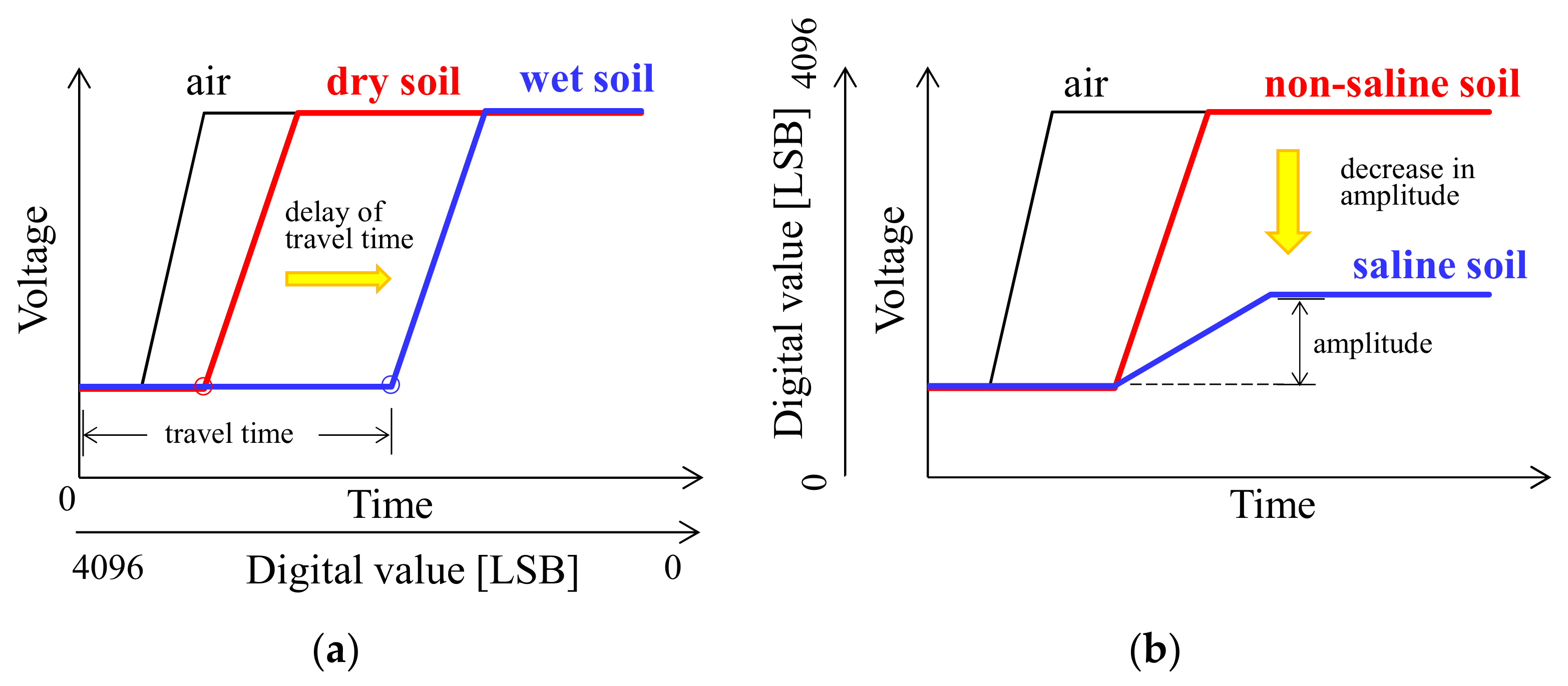
2.2.1. Relationship between the Sensor Outputs and the Dielectric Constant/Matric Potential

TDR and TDT determine ε_b and convert it to θ using an empirically obtained relationship explained by Topp et al. [36]. Although this empirically obtained relationship can be applied to most soils, the relationship is soil-specific and does not work for some soils [37]. Therefore, it is more effective to convert the sensor output to ε_b instead of θ and use the conversion best suited for field soil.

The relationship between the sensor output t_D and ε_b and that between the sensor output C_D and ψ (kPa) were obtained simultaneously from a single experiment by comparing the sensor outputs with the reference sensors. The reference sensors were commercially available TDT sensors (SDI-12 soil moisture, Acclima, Meridian, ID, USA) and ψ sensors (ML-2600AES tensiometer, mol, Tokyo, Japan; MPS-6, Meter Group, Pullman, WA, USA). The proposed and reference sensors were placed in a plastic box with an inner length, width, and height of 30 cm, 20 cm, and 10 cm, respectively. Three sets of sensors and three plastic containers were used. The boxes were filled with three soils to confirm that the relationships were independent of the soil type. Toyoura sand, a soil collected from the Gifu University experimental field (hereafter, GU soil), and Andisol, whose textures were sand, sandy clay loam, and sandy loam, respectively. The soil texture, bulk density, and saturated hydraulic conductivity of each soil sample are listed in

Table 1. Sand, silt, and clay percentages, soil organic matter (SOM) content, bulk density, and hydraulic conductivity of Toyoura sand, soil collected from the Gifu University experimental field (GU soil), and Andisol.

	% Sand	% Silt	% Clay	SOM Content (kg kg−1)	Bulk Density (kg m−3)	Hydraulic Conductivity (m s−1)
Toyoura sand	100.0	0.0	0.0	0.00	1340	1.2 × 10−4
GU soil	61.7	16.1	22.2	0.07	1080	1.5 × 10−5
Andisol	66.3	27.5	6.2	0.23	820	4.5 × 10−6

. GU soil contains a relatively large ratio of clay, whereas Andisol is a volcanic soil with a significant soil organic matter (SOM) content and a small bulk density. The soils were initially saturated and air-dried at a constant temperature of 20 °C. An electric fan was used to blow air across the soil surface to enhance the soil water evaporation. The control and data storage of the new sensor were conducted using a personal computer. A datalogger (CR1000, Campbell Scientific, Logan, UT, USA) was used for data collection from the SDI-12 soil moisture and tensiometer, and a datalogger (ZL6, Meter Group) was used for data collection from the MPS-6. The experiment was performed for 21 days, and each sensor measurement was performed every hour. The ε_b measured with the SDI-12 soil moisture and the ψ measured with the tensiometer and MPS-6 were compared with the sensor outputs t_D and C_D to establish the relationships.

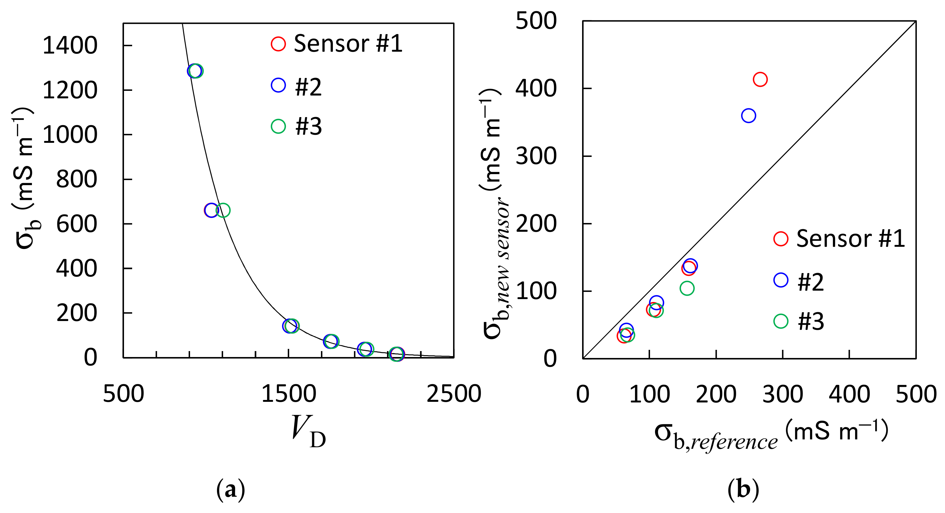
2.2.2. Relationship between Sensor Output and Electrical Conductivity

The calibration of the proposed sensor for σ_b was performed using measurements conducted in KCl solution. The sensor was placed in a plastic column with an inner diameter of 15 cm and a height of 18 cm. The column was filled with 0.0001 mol L⁻¹, 0.00025 mol L⁻¹, 0.005 mol L⁻¹, 0.01 mol L⁻¹, 0.05 mol L⁻¹, and 0.1 mol L⁻¹ concentrations of KCl solution, and new sensor measurements were performed in each solution. The electrical conductivity of each solution (mS m⁻¹) was measured using a multiple water quality meter (MM-60R, DKK-TOA, Tokyo, Japan). The measurement results were then compared with the output value V_D of the new sensor.

An additional experiment was conducted with KCl solution containing Toyoura sand to confirm that the calibration equation obtained from the above experiment with KCl solutions works for soil. The sensor was fixed in space within a plastic column (with an inner diameter of 8.3 cm and a height of 17 cm) filled with sand. The concentration of KCl solution was set at 0.1 mol L⁻¹, and a known amount of KCl solution was added to the sand to achieve θ values of 0.15 m³ m⁻³, 0.20 m³ m⁻³, 0.25 m³ m⁻³, and 0.30 m³ m⁻³. The new sensor measurements were performed for each soil sample with a different θ value, and the sensor outputs were converted to σ_b using the calibration equation obtained from the above experiment (Equation (5)). Furthermore, the electrical conductivity of the KCl solution was measured using the MM-60R, and the σ_b of the sand (mS m⁻¹) was calculated using the equation proposed by Hilhorst et al. [38]:

$${\mathsf{\sigma }}_{\mathrm{b}}=\frac{{\mathsf{\sigma }}_{\mathrm{w}}\left({\mathsf{\epsilon }}_{\mathrm{b}}-{\mathsf{\epsilon }}_0\right)}{{\mathsf{\epsilon }}_{\mathrm{w}}}$$

(1)

where σ_w is the electrical conductivity of the KCl solution (mS m⁻¹), ε_b is the dielectric constant of the soil, ε₀ is the dielectric constant of the soil when its electrical conductivity is zero (which can be treated as that of oven-dry soil), and ε_w is the dielectric constant of water (≈80). The ε_b values were calculated backward from the θ value using Topp’s equation [36].

$$\mathsf{\theta }=4.3\times {10}^{-6}{\mathsf{\epsilon }}_{\mathrm{b}}{}^3-5.5\times {10}^{-4}{\mathsf{\epsilon }}_{\mathrm{b}}{}^2+2.92\times {10}^{-2}{\mathsf{\epsilon }}_{\mathrm{b}}-5.3\times {10}^{-2}$$

(2)

The ε₀ value was calculated using Equation (2) for θ = 0. Furthermore, we compared the σ_b measured using the proposed sensor with that calculated using Equation (1).

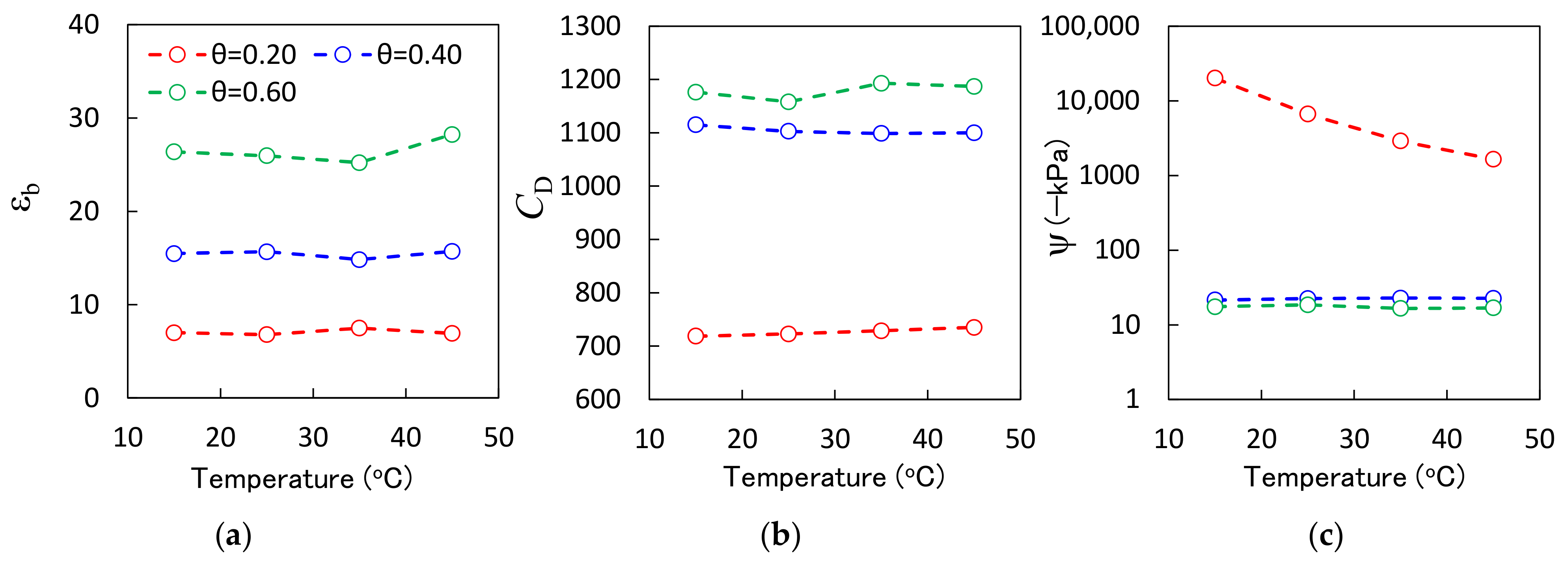
2.3. Evaluation of Temperature Dependence of Sensor Outputs

The temperature dependence of soil sensors is often a problem owing the dynamics of soil temperature variation. The temperature dependence of the proposed and reference sensors was evaluated in a laboratory experiment. The new sensor, SDI-12 soil moisture, and MPS-6 were placed in plastic boxes with an inner length, width, and height of 30 cm, 20 cm, and 10 cm, respectively, and these were filled with Andisol with θ values of 0.20 m³ m⁻³, 0.40 m³ m⁻³, and 0.60 m³ m⁻³. Each plastic box was placed in a constant-temperature chamber, and the temperature was increased from 15 °C to 45 °C in 10 °C increments. We increased the chamber temperature when the sensor thermistor temperature reached the set chamber temperature. Each sensor was measured before changing the chamber temperature.

2.4. In Situ Sensor Evaluation

The in situ sensor performance evaluation was conducted in an experimental field at Gifu University (35°46′19.17″ N, 136°73′93.25″ E). The experimental field was maintained in bare soil. The proposed sensor was inserted at depths of 10 cm and 20 cm. The sensor board was placed perpendicular to the ground surface to prevent the obstruction of water and heat flow. The two sensors were connected to wireless communication modules (LoRa module), which sent the measured data to the master node located 40 m away from the field via LoRa communication. The master node then uploaded the data to the cloud via cell phone communication. A weather station (ATMOS 41, Meter Group) and a ZL6 datalogger were installed in the field to obtain weather data. New sensor and weather station data were collected every 15 min. The in situ evaluation began on 1 July 2021 and continued until 26 January 2022. A liquid nitrogen fertilizer was applied to the field on 11 November to determine whether the new sensor could capture an increase in σ_b caused by the liquid fertilizer.

3. Results and Discussion

3.1. Sensor Calibration

3.1.1. Relationship between Sensor Output and Dielectric Constant

The relationship between the t_D of the new sensor and the ε_b measured with the SDI-12 soil moisture is shown in Figure 3a. The different colored plots represent the different soil types. The ε_b value of each soil showed ranges of 4–25, 6–32, and 9–38 for the Toyoura sand, GU soil, and Andisol, respectively. The associated t_D values were distributed between 2590 and 3290. Although a minor difference was observed in the ε_b ranges, the relationship between t_D and ε_b was consistent for all soils. Therefore, the relationship was independent of the soil type. We approximated this relationship using the following cubic equation:

$${\mathsf{\epsilon }}_{\mathrm{b}}=-3.96\times {10}^{-8}{t}_{\mathrm{D}}{}^3+3.93\times {10}^{-3}{t}_{\mathrm{D}}{}^2-1.33t_{\mathrm{D}}+1521.82$$

(3)

The coefficient of determination R² for Equation (3) was 0.98. Figure 3b compares the ε_b values determined using the reference and proposed sensors. The two values were consistent and distributed around the 1:1 line. Slight errors were observed when the θ of each soil was relatively large because of the non-uniform distribution of water in the soil after the initial saturation process. Furthermore, the drying process may have homogenized the variation in the θ distribution, which resulted in better agreement at small θ values. The root-mean-square error (RMSE) and mean absolute percentage error (MAPE) were 1.74% and 6.7%, respectively. The output t_D of the proposed sensor can be converted to ε_b using Equation (3). The θ can be calculated from the ε_b by selecting an appropriate equation from the literature; for example, Topp et al.’s equation [36] can be used for most mineral soils and Miyamoto et al.’s equation [37] can be used for volcanic ash soils. Deriving a soil-specific equation to convert ε_b to θ will result in the best accuracy.

3.1.2. Relationship between Sensor Output and Matric Potential

Figure 4a shows the relationship between the C_D of the proposed sensor and the ψ measured using a tensiometer and an MPS-6. The tensiometer and MPS-6 had measurable ranges of ψ. We used the tensiometer-measured ψ larger than −100 kPa and MPS-6-measured ψ smaller than −100 kPa as the reference values. The C_D value of the proposed sensor and the reference sensor-measured ψ values did not respond to soil drying, that is, they were almost constant, in Toyoura sand. It is reportedly challenging to maintain a hydraulic connection to the pore water in course soil using the ψ sensors in porous media [26,28], and the same phenomenon occurred in the Toyoura sand. Therefore, Figure 4a only shows the results for the GU soil and Andisol. The C_D values were initially constant when the soil was wet (the ψ was greater than −5 kPa) before dynamically decreasing when the ψ reached −5 kPa as a result of drying. The C_D decreased continuously until the ψ reached −100 kPa. However, the C_D value decreased only slightly after the ψ reached −100 kPa. A minor difference was observed between the results from the two soils when the ψ was less than −100 kPa. Except for the previously mentioned loss of hydraulic connections in sand, ψ sensors are unlikely to exhibit soil dependence in porous media. Therefore, this difference may be because of individual sensor variability caused by minor differences in the ceramic plate structure and contact between the ceramic plate and the capacitance. Because the relationship between C_D and ψ is similar to the soil water retention curve, which represents the relationship between θ and ψ, we used the modified van Genuchten model [39], which is a commonly used model for soil water retention curves, to express these relationships:

$$\mathsf{\psi }=-\frac{1}{\mathsf{\alpha }}{\left[{\left(\frac{C_{\mathrm{D}}-C_{\mathrm{D}, \min }}{C_{\mathrm{D},\max }-C_{\mathrm{D},\min }}\right)}^{\frac{n}{1-n}}-1\right]}^{1/n}$$

(4)

where C_D,max and C_D,min are the maximum and minimum values of C_D, respectively, and α and n are curve shape factors. The four parameters obtained by the fitting are listed in

Table 2. Obtained parameters for the modified van Genuchten model that expresses the relationships between the capacitance digital value and the matric potential of the new sensor (Equation (4)). The parameters for the Gifu University experimental field soil (GU soil), the Andisol, and both soils (all plots) are shown.

	CD,max	CD,min	α (kPa−1)	n
GU soil	1357	715	0.086	2.32
Andisol	1415	743	0.100	2.11
All plots	1415	715	0.105	2.04

. For the C_D,max and C_D,min values, we selected the maximum and minimum C_D values measured in the respective soils. The parameters of the two sensors in the GU soil and the Andisol were different in that the GU soil sensor showed lower values for the same potential below −100 kPa and above −10 kPa. Therefore, while it would be desirable to obtain sensor-specific parameters for each sensor by calibration, it requires considerable effort. Additionally, little variation was observed in the range of −100 kPa to −10 kPa, which is the dominant range in the actual field. Therefore, the common parameters for all the sensors were derived by fitting all the data plots. In this case, the minimum and maximum values measured in the two soils were selected for C_D,max and C_D,min.

Figure 4b compares the ψ values determined with the new sensor and Equation (4) to the reference values. The two ψ values were consistent between −100 to −10 kPa, whereas the new sensor overestimated the ψ when the ψ was smaller than −100 kPa because the changes in the C_D values become smaller when the ψ < −100 kPa compared with those when the ψ > −100 kPa. However, the ψ range in the field is generally greater than −100 kPa. Therefore, we can conclude that the new sensor performs very well. The ψ values determined with the sensor-specific parameters and those determined with the common parameters were consistent when the ψ was above −100 kPa. While the errors with the common parameters increased when the GU soil was below −100 kPa, they decreased for the Andisol, which we considered to be coincidental. The ψ varies in order scale, so that the RMSEs of the logarithmic values of ψ were calculated. The RMSE was 0.57 for the GU soil with the soil-specific parameters, 0.60 for the Andisol with the soil-specific parameters, 0.88 for the GU soil with the common parameters, and 0.05 for the Andisol with the common parameters. The new sensors can measure the ψ between −10,000 kPa and −10 kPa, and the accuracy of the ψ measurements was particularly good between −100 kPa and −10 kPa.

In this study, we calibrated the new ψ sensor by comparing it with a commercialized ψ sensor (an MPS-6) during the soil air-drying process. Although this method is simple, it has certain disadvantages, such as the time-consuming nature of the soil air-dying process and the measurement errors of commercial sensors. Thus, sensor calibration with a pressure plate apparatus such as the one used by Noborio et al. [26] may yield better results.

3.1.3. Relationship between Sensor Output and Electrical Conductivity

The relationship between the V_D and σ_b for the KCl solutions is shown in Figure 5a. The σ_b values of the 0.1 mol L⁻¹, 0.05 mol L⁻¹, 0.01 mol L⁻¹, 0.005 mol L⁻¹, 0.00025 mol L⁻¹, and 0.00010 mol L⁻¹ KCl solutions measured with the multiple water quality meter were 1285 mS m⁻¹, 661 mS m⁻¹, 140 mS m⁻¹, 72 mS m⁻¹, 37 mS m⁻¹, and 1 mS m⁻¹, respectively. The V_D values decreased as the σ_b increased, and the relationship between the V_D and σ_b was expressed as an exponential function (denoted by the solid line in Figure 5a):

$${\mathsf{\sigma }}_{\mathrm{b}}=2.92\times {10}^4\exp \left(-3.46\times {10}^{-3}{V}_D\right)$$

(5)

The R² for Equation (5) was 0.98. Notably, the ε_b values were also measured using the proposed sensor during the experiment, and it was found that the ε_b values were almost 80 (εb of water) for the 0.01 mol L⁻¹, 0.005 mol L⁻¹, 0.00025 mol L⁻¹, and 0.00010 mol L⁻¹ KCl solutions, but greater than 90 for the 0.1 mol L⁻¹ and 0.05 mol L⁻¹ KCl solutions. Furthermore, TDR sometimes fails to accurately determine the ε_b in large σ_b materials because the decrease in voltage amplitude causes ambiguous travel times (see Figure 2) [40]. The TDT system implemented in this study encountered a similar problem.

Figure 5b compares the σ_b values of the Toyoura sand determined using Equation (1), which is assumed to be a reference, and those determined using the new sensor and Equation (5). The σ_b value increased from 61 mS m⁻¹ to 266 mS m⁻¹ as the θ increased. The reference and proposed sensor-determined σ_b values were consistent at σ_b values smaller than 200 mS m⁻¹, whereas the larger σ_b values were slightly overestimated by the proposed sensor. However, the reference σ_b values that were determined using the Hilhorst model were not necessarily accurate since the Hilhorst model is less accurate at high salinity [38,41]. Therefore, it cannot be judged whether the sensor overestimated the value or whether the reference values were too small. The RMSE was 62 mS m⁻¹. Although the large σ_b values were mismatched, the new sensor can determine the σ_b value of the soil with sufficient accuracy.

3.2. Temperature Dependence

Figure 6 shows the ε_b, C_D, and ψ values of the proposed sensor as functions of the temperature. The ε_b values measured with the new sensor varied slightly with temperature. However, there was no clear trend (Figure 6a). For example, the ε_b value of θ = 0.60 m³ m⁻³ Andisol decreased from 26.3 to 25.2 as the temperature increased from 15 °C to 35 °C, but increased to 28.3 as the temperature increased from 35 °C to 45 °C. The dielectric constant of water decreased as the temperature increased [15]. In addition, Andisol is known to have large amounts of bound water, which is strongly adsorbed by the soil particles. Bound water therefore has a lower dielectric constant value compared with free water [42]. The ratio between this bound water and free water in the soil pores is partly controlled by the temperature [43]. Moreover, it is possible that water redistribution in the container may have influenced the measurements, thereby resulting in a complicated trend in the effects of the temperature on the ε_b. Although the ε_b showed a complex temperature dependence, the ε_b fluctuation was at most 3.1, whereas the equivalent change in the θ calculated using Equation (2) was only 0.028 m³ m⁻³. Therefore, the temperature dependence of the ε_b need not be considered.

As the temperature increased, the C_D value of θ = 0.20 m³ m⁻³ Andisol increased from 719 to 735, and that of θ = 0.40 m³ m⁻³ Andisol decreased from 1115 to 1110. The ψ converted from C_D showed little change for θ = 0.40 m³ m⁻³ and θ = 0.60 m³ m⁻³ Andisol (Figure 6c). The fluctuation in the ψ in these soils was less than 2 kPa. However, the ψ value of θ = 0.20 m³ m⁻³ showed a dynamic increase from −20,133 kPa to −1649 kPa as the temperature increased, although the C_D value showed a slight increase because the minor temperature dependence of the C_D value is amplified by conversion using Equation (4) when the ψ is small, that is, when the soil water content is small. A similar phenomenon was reported for the MPS-6 [20], and it is a common weakness of capacitance and porous medium-based ψ sensors. Therefore, the temperature dependency of the ψ must be considered when a sensor is used in dry conditions.

3.3. Field Evaluation

Figure 7 shows the in situ soil temperature, θ, ψ, and σ_b measured with the proposed sensor. The θ was calculated using Equations (2) and (3), and the ψ and σ_b were calculated using Equations (4) and (5), respectively. The parameters were determined from all the plots (Table 2). The sensors were installed at depths of 10 cm and 20 cm. The 20 cm depth sensor showed missing data from 18 August to 12 October 2021 and from 27 December 2021 to 7 January 2022 owing a malfunction of the wireless communication module. The 10 cm sensor, whose communication module functioned correctly, performed measurements throughout the period without any data loss. While the communication stability is an issue for future consideration, the sensor itself was stable and could perform measurements for a long period.

The soil temperature at depths of 10 cm and 20 cm showed fluctuations similar to those of the air temperature, which gradually decreased from approximately 40 °C to 5 °C from July to January. The temperature 10 cm from the soil surface had a larger amplitude compared with that at a 20 cm depth. The θ ranged between 0.18 m³ m⁻³ and 0.41 m³ m⁻³ throughout the experimental period, increasing with rainfall and decreasing with evaporation and infiltration. The value at 20 cm was approximately 0.05 m³ m⁻³ higher than that at 10 cm because a depth of only 10 cm was more likely to be affected by surface evaporation and rainfall drainage. The ψ varied from −2 to −103 kPa and increased to a value near zero immediately after rainfall before decreasing during subsequent drying. The ψ rarely fell below −100 kPa. As for the soil water content, the soil at a depth of 10 cm was more prone to drying compared with that at a depth of 20 cm, which indicated a lower matric potential. The σ_b ranged between 11 mS m⁻¹ and 33 mS m⁻¹, and the trend was similar to that of the soil water content. These results are satisfactory because the σ_b is controlled in part by the θ. The effect of liquid fertilizer applied on 11 November was difficult to determine because of the strong influence of the θ on the σ_b. However, the decrease in the σ_b at a depth of 10 cm immediately after 11 November was milder than that during a similar drying process. Additionally, the σ_b at a 20 cm depth remained high from 22 November to 6 December, but a sudden decrease on 6 December was observed following rainfall owing to liquid fertilizer transport in the soil. As described above, the new sensor accurately captured phenomena in the field and, hence, can be considered to provide highly reliable data.

Because the new sensor can determine the θ and ψ in the field simultaneously, it can obtain the in situ soil water retention curve, shown in Figure 8. The curves for each depth were constructed for two different periods: summer (from 1 July to 18 August 2021) and fall (from 12 October to 27 December 2021). At a depth of 10 cm, the θ varied from 0.19 m³ m⁻³ to 0.37 m³ m⁻³ and the ψ varied from −70 kPa to −3 kPa with wetting and drying. At a depth of 20 cm, the θ varied from 0.24 m³ m⁻³ to 0.41 m³ m⁻³ and the ψ varied from −103 kPa to −3 kPa. The θ decreased slightly at a depth of 20 cm after reaching 0.25 m³ m⁻³, whereas the ψ kept decreasing relatively dynamically. Such a difference between the 10 cm and 20 cm depths can be attributed to the compaction and distance from the surface. These results show that ψ is a better indicator of soil dryness than θ. Furthermore, dynamic hysteresis was observed during the summer at a depth of 10 cm, but was rarely observed at a depth of 10 cm in the fall. However, hysteresis was not observed at a depth of 20 cm because of the rapid drying speed of the 10 cm soil layer in the summer, which is associated with high air temperature and intensive solar radiation. This rapid drying leaves more isolated water in the soil at the same ψ. The in situ soil water retention curves differ from those obtained in the laboratory [44] and provide essential information for estimating soil water movement in the field.

4. Conclusions

This study proposed a new TDT-based sensor that can simultaneously determine the soil water content (θ), matric potential (ψ), electrical conductivity (σ_b), and temperature for application in smart farming. A series of laboratory and field tests were conducted to evaluate the performance of the proposed sensor. Laboratory tests revealed the relationships between the digital values of the sensor outputs and the soil properties, as well as the temperature dependence of the sensor outputs. The field test measured the transient soil conditions using the sensor for a relatively long period. The results indicated that the sensor provides satisfactory performance with acceptable accuracy, small temperature dependence, and a long lifetime. Additionally, the proposed sensor can provide vital information for the in situ soil water retention curve owing to its ability to simultaneously determine θ and ψ. We believe that the novel sensor proposed in this study can contribute to a wide range of studies on topics including smart farming, soil mass, and heat transfer.

References

1. Wolfert, S.; Ge, L.; Verdouw, C.; Bogaarrdt, M.-J. Big data in smart farming—A review. Agric. Syst. 2017, 153, 69–80. [Google Scholar] [CrossRef]
2. Ritchie, J.T.; Nesmith, D.S. Temperature and crop development. In Modeling Plant and Soil Systems; Hanks, J., Ritchie, J.T., Eds.; ASA-CSSA-SSSA: Madision, WI, USA, 1991; pp. 5–29. [Google Scholar]
3. Fares, A.; Alva, A.K. Evaluation of capacitance probes for optimal irrigation of citrus through soil moisture monitoring in an entisol profile. Irrig. Sci. 2000, 19, 57–64. [Google Scholar] [CrossRef]
4. Vellidis, G.; Tucker, M.; Perry, C.; Kvien, C.; Bednarz, C. A real-time wireless smart sensor array for scheduling irrigation. Comput. Eectron. Agr. 2008, 61, 44–50. [Google Scholar] [CrossRef]
5. Kim, Y.; Evan, R.G.; Iverson, W.M. Remote sensing and control of an irrigation system using a distributed wireless sensor network. IEEE T. Instrum. Meas. 2008, 57, 1379–1387. [Google Scholar]
6. Noborio, K.; McInnes, K.J.; Heilman, J.L. Two-dimensional model for water, heat, and solute transport in furrow-irrigated soil: II. field evaluation. Soil Sci. Soc. Am. J. 1996, 60, 1010–1021. [Google Scholar] [CrossRef]
7. Walczak, A.; Lipiński, M.; Janik, G. Application of the TDR sensors and the parameters of injection irrigation for the estimation of soil evaporation intensity. Sensors 2021, 21, 2309. [Google Scholar] [CrossRef]
8. Coelho, E.F.; Or, D. Root distribution and water uptake patterns of corn under surface and subsurface drip irrigation. Plant Soil 1999, 206, 123–136. [Google Scholar] [CrossRef]
9. Kojima, Y.; Shigeta, R.; Miyamoto, N.; Shirahama, Y.; Nishioka, K.; Mizoguchi, M.; Kawahara, Y. Low-cost soil moisture profile probe using thin-film capacitors and a capacitive touch sensor. Sensors 2016, 16, 1292. [Google Scholar] [CrossRef]
10. Kizito, F.; Campbell, C.S.; Campbell, G.S.; Cobos, D.R.; Teare, B.L.; Carter, B.; Hopmans, J.W. Frequency, electrical conductivity and temperature analysis of a low-cost capacitance soil moisture sensor. J. Hydrol. 2008, 352, 367–378. [Google Scholar] [CrossRef]
11. Seyfried, M.S.; Murdock, M.D. Response of a new soil water sensor to variable soil, water content, and temperature. Soil Sci. Soc. Am. J. 2001, 65, 28–34. [Google Scholar] [CrossRef] [Green Version]
12. Corwin, D.L.; Lesch, S.M. Apparent soil electrical conductivity measurements in agriculture. Comput. Electron. Agr. 2005, 46, 11–43. [Google Scholar] [CrossRef]
13. Crowin, D.L.; Lesch, S.M. Application of soil electrical conductivity to prevision agriculture: Theory, principles, and guidelines. Agron. J. 2003, 95, 455–471. [Google Scholar]
14. Rhodes, J.D. Electrical conductivity methods for measuring and mapping soil salinity. Adv. Agron. 1993, 49, 201–251. [Google Scholar]
15. Noborio, K. Measurement of soil water content and electrical conductivity by time domain reflectometry: A review. Comput. Electron. Agr. 2001, 31, 213–237. [Google Scholar] [CrossRef]
16. Robinson, D.A.; Jones, S.B.; Wraith, J.M.; Or, D.; Friedman, S.P. A review of advances in dielectric and electrical conductivity measurement in soils using time domain reflectometry. Vadose Zone J. 2003, 2, 444–475. [Google Scholar] [CrossRef]
17. Rhoades, J.D. Inexpensive four-electrode probe for monitoring soil salinity. Soil Sci. Soc. Am. J. 1979, 43, 817–818. [Google Scholar] [CrossRef]
18. Konukcu, F.; Gowing, J.W.; Rose, D.A. Simple sensors to achieve fine spatial resolution in continuous measurements of soil moisture and salinity. Hydrol. Earth Syst. Sci. 2002, 6, 1043–1051. [Google Scholar] [CrossRef]
19. Hillel, D. Environmental Soil Physics; Academic Press: London, UK, 1998; pp. 129–172. [Google Scholar]
20. Kojima, Y.; Noborio, K.; Mizoguchi, M.; Kawahara, K. Matric potential sensor using dual probe heat pulse technique. Agr. Info. Res. 2017, 26, 77–85. [Google Scholar] [CrossRef] [Green Version]
21. Richards, L.A. Soil moisture tensiometer materials and construction. Soil Sci. 1942, 53, 241–248. [Google Scholar] [CrossRef] [Green Version]
22. Dabach, S.; Shani, U.; Lazarovitch, N. Optimal tensiometer placement for high-frequency subsurface drip irrigation management in heterogeneous soils. Agr. Water Manag. 2015, 152, 91–98. [Google Scholar] [CrossRef]
23. Walthert, L.; Schleppi, P. Equations to compensate for the temperature effect on readings from dielectric Decagon MPS-2 and MPS-6 water potential sensors in soils. J. Plant Nutr. Soil Sci. 2018, 181, 749–759. [Google Scholar] [CrossRef]
24. Da Mota, W.N.; Evangelista, A.W.P.; Maia, L.J.Q.; Correchel, V.; Alves, J.; Varrone, L.F.R.; de F.N. Gitirana, G., Jr. Development of a heat pulse sensor for measuring matric suction on soilless substrates. Comput. Electron. Agr. 2021, 185, 106119. [Google Scholar] [CrossRef]
25. Or, D.; Wraith, J.M. A new soil matric potential sensor based on time domain reflectometry. Water Resour. Res. 1999, 35, 3399–3407. [Google Scholar] [CrossRef]
26. Noborio, K.; Horton, R.; Tan, C.S. Time domain reflectometry probe for simultaneous measurement of soil matric potential and water content. Soil Sci. Soc. Am. J. 1999, 63, 1500–1505. [Google Scholar] [CrossRef]
27. Vaz, C.M.P.; Hopmans, J.W.; Macedo, A.; Bassoi, L.H.; Wildenschild, D. Soil water retention measurements using a combined tensiometer-coiled time domain reflectometry probe. Soil Sci. Soc. Am. J. 2002, 66, 1752–1759. [Google Scholar] [CrossRef] [Green Version]
28. Kojima, Y.; Kawashima, T.; Noborio, K.; Kamiya, K.; Horton, R. A dual-probe heat pulse-based sensor that simultaneously determine soil thermal properties, soil water content and soil water matric potential. Comput. Electron. Agr. 2021, 188, 106331. [Google Scholar] [CrossRef]
29. Campbell, G.S.; Calissendorff, C.; Williams, J.H. Probe for measuring soil specific heat using a heat-pulse method. Soil Sci. Soc. Am. J. 1991, 55, 291–293. [Google Scholar] [CrossRef] [Green Version]
30. Bristow, K.L.; Kluitenberg, G.J.; Horton, R. Measurement of soil thermal properties with a dual-probe heat-pulse technique. Soil Sci. Soc. Am. J. 1994, 58, 1288–1294. [Google Scholar] [CrossRef]
31. Topp, G.C.; Lapen, D.R.; Edwards, M.J.; Young, G.D. Laboratory calibration, in-field validation and use of a soil penetrometer measuring cone resistance and water content. Vadose Zone J. 2003, 2, 633–641. [Google Scholar] [CrossRef]
32. Miyamoto, H.; Ito, N.; Yasunaga, E.; Takaichi, S.; Mase, A.; Chikushi, J. Measurement of dielectric properties using time domain transmissiometry (TDT) with broad band impulse-signal. J. Jpn. Soc. Soil Phys. 2008, 110, 3–12. (In Japanese) [Google Scholar]
33. Harlow, R.C.; Burke, E.J.; Ferré, T.P.A.; Bennett, J.C.; Shuttleworth, W.J. Measuring spectral dielectric properties using gated time domain transmission measurements. Vadose Zone J. 2003, 2, 424–432. [Google Scholar] [CrossRef]
34. Miyamoto, H.; Ito, N.; Mase, A.; Tokumoto, I.; Chikushi, J. Application of time domain transmissiometry to coupled measurements of soil moisture and electrical conductivity. IDRE Journal 2013, 288, 25–31. (In Japanese) [Google Scholar]
35. Blonquist, J.M.; Jones, S.B.; Robinson, D.A. A time domain transmission sensor with TDR performance characteristics. J. Hydrol. 2005, 314, 235–245. [Google Scholar] [CrossRef]
36. Topp, G.C.; Davis, J.L.; Annan, A.P. Electromagnetic determination of soil water content: Measurements in coaxial transmission lines. Water Resour. Res. 1980, 16, 574–582. [Google Scholar] [CrossRef] [Green Version]
37. Miyamoto, T.; Kobayashi, R.; Annaka, T.; Chikushi, J. Applicability of multiple length TDR probes to measure water distributions in and Andisol under different tillage systems in Japan. Soil Till. Res. 2001, 60, 91–99. [Google Scholar] [CrossRef]
38. Hilhorst, M.A. A pore water conductivity sensor. Soil Sci. Soc. Am. J. 2000, 64, 1922–1925. [Google Scholar] [CrossRef] [Green Version]
39. Van Genuchten, M.T. A closed-form equation for predicting the hydraulic conductivity of unsaturated soils. Soil Sci. Soc. Am. J. 1980, 44, 892–898. [Google Scholar] [CrossRef] [Green Version]
40. Jones, S.B.; Or, D. Frequency domain analysis for extending time domain reflectometry water content measurement in highly saline soils. Soil Sci. Soc. Am. J. 2004, 68, 1568–1577. [Google Scholar] [CrossRef] [Green Version]
41. Zemni, N.; Bouksila, F.; Slama, F.; Persson, M.; Berndtsson, R.; Bouhlila, R. Evaluation of modified Hilhorst models for pore electrical conductivity estimation using a low-cost dielectric sensor. Arab. J. Geosci. 2022, 15, 1089. [Google Scholar] [CrossRef]
42. Miyamoto, T.; Annaka, T.; Chikushi, J. Extended dual composite sphere model for determining dielectric permittivity of Andisols. Soil Sci. Soc. Am. J. 2005, 69, 23–29. [Google Scholar] [CrossRef]
43. Wraith, J.M.; Or, D. Temperature effects on soil bulk dielectric permittivity measured by time domain reflectometry: Experimental evidence and hypothesis development. Water Resour. Res. 1999, 35, 361–369. [Google Scholar] [CrossRef]
44. Bordoni, M.; Bittelli, M.; Valentino, R.; Chersich, S.; Meisina, C. Improving the estimation of complete field soil water characteristic curves through field monitoring data. J. Hydrol. 2017, 552, 283–305. [Google Scholar] [CrossRef]
Figure 1. (a) Schematic and (b) photograph of the proposed sensor.
Sensors 23 02340 g001
Figure 2. Time domain transmissiometry waveform analysis for (a) soil water content (dielectric constant) and (b) electrical conductivity.
Sensors 23 02340 g002
Figure 3. (a) Relationship between dielectric constant (εb) measured with a reference sensor and tD measured with the new sensor, and (b) comparison between εb measured with the reference sensor (εb, reference) and the new sensor (εb, new sensor). The different colored plots represent the different soil types, i.e., Toyoura sand, Gifu University experimental field soil (GU soil), and Andisol.
Sensors 23 02340 g003
Figure 4. (a) Relationship between the soil matric potential (ψ) and the CD measured using the reference and proposed sensors, respectively, and (b) comparison between the ψ measured with the reference sensor (ψreference) and the proposed sensor (ψnew sensor). The different colored plots in panel (a) represent the Gifu University experimental field soil (GU soil) and the Andisol, and the solid lines indicate fitted models (Equation (4)) with the plots of either soil and with all plots. The different colored plots in panel (b) represent the GU soil and the Andisol with the sensor-specific (SS) or common (C) parameters of Equation (4).
Sensors 23 02340 g004
Figure 5. (a) Relationship between the electrical conductivity (σb) of potassium chloride (KCl) solution measured with the reference sensor and the VD measured with the proposed sensor, and (b) comparison between the σb of the Toyoura sand calculated with Equation (1) (σb,reference) and the σb determined using the proposed sensor (σb,new sensor). The different colored plots represent different sensor numbers.
Sensors 23 02340 g005
Figure 6. (a) The new sensor-measured dielectric constant (εb), (b) digital values of the new sensor-measured capacitance (CD), and (c) the new sensor-measured matric potential (ψ) as functions of the temperature. The colored plot indicates the different water content (θ) of the Andisol, i.e., 0.20 m3 m−3, 0.40 m3 m−3, and 0.60 m3 m−3.
Sensors 23 02340 g006
Figure 7. (a) Time series of soil properties measured with the new sensor in the Gifu University experimental field. The panels present (a) soil and air temperatures, (b) soil volumetric water content and precipitation, (c) soil matric potential, and (d) soil bulk electrical conductivity. The “LF” in panel (d) indicates liquid fertilizer application.
Sensors 23 02340 g007
Figure 8. In situ water retention curves were obtained with the new sensors installed at depths of (a) 10 cm and (b) 20 cm. The different colored plots indicate the different periods: summer (from 1 July to 18 August 2021) and fall (from 12 October to 27 December 2021).
Sensors 23 02340 g008