

T-RAIM Approaches: Testing with Galileo Measurements


Abstract
1. Introduction
- Using a performance-based approach to give the manufacturer’s the freedom of implementation;
- Static receiver and dynamic receiver options: considering the cases with and without known receiver position.
2. Timing Solution
2.1. Timing Solution Estimation
2.2. Integrity Algorithms
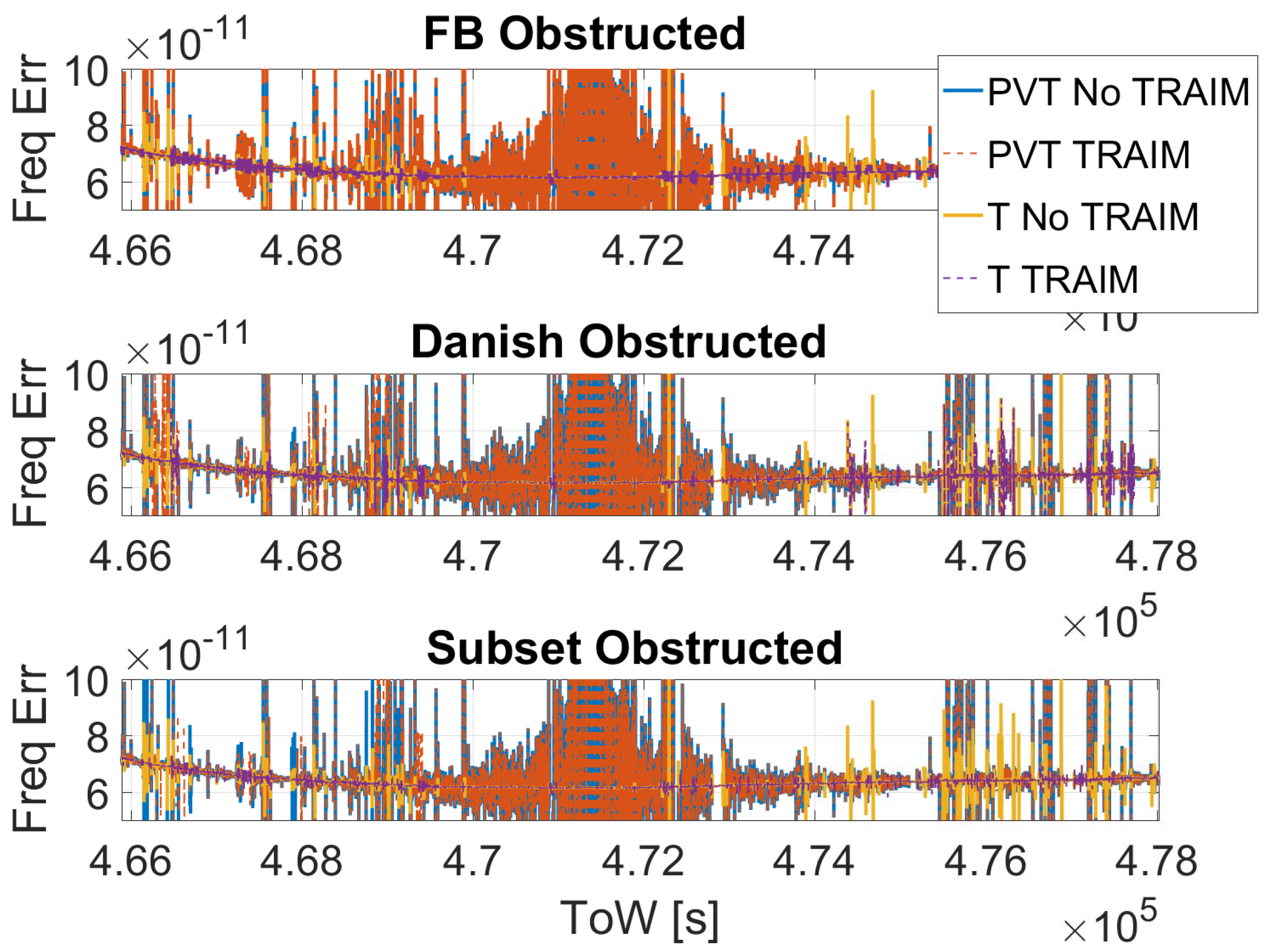
2.2.1. Forward-Backward
- Geometry; the system is not robust enough to support integrity checks;
- Inconsistency between GT and LT; GT detects an inconsistency among the measurements set but all the measurements pass the LT;
- Separability; LT identifies a measurement as an outlier but it is too correlated with other measurements and it is not possible to identify the real outlier.
2.2.2. Danish
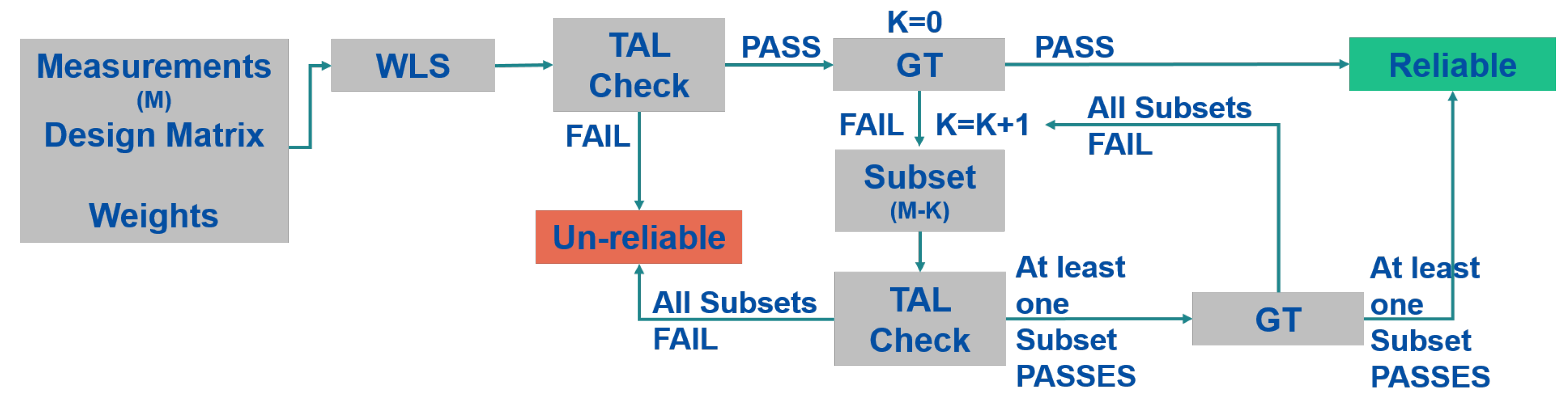
2.2.3. Subset
3. Performance Metrics
- Reliable availability, defined as: the percentage of time in which the timing solution is declared reliable by the integrity algorithm. The reliable availability is computed as:where is the number of the reliable epochs, and is the total number of epochs of the dataset.
- Frequency error: represents the variations of a timing signal generated by a clock. Here the frequency error is estimated from the receiver clock bias estimation according to the method described in Ref. [21]. The frequency error is computed as:where is the normalized frequency error at the epoch t, is the receiver clock bias estimation in seconds, K is an integer, and is the averaging time interval.in which is the sampling rate of the receiver clock bias.
- Allan Deviation: the square root of the Allan variance, which is a generalization of the sample variance and is commonly used to characterize the stability of oscillators [31]. This parameter provides indications about the expected frequency deviation that can occur in the averaging time interval, [32]. Additional details for the ADEV estimation using GNSS measurements are available in Ref. [21].
- Execution time: the time needed to execute the algorithm. In particular, the total execution time (the time needed for processing the whole dataset) and the single epoch execution time are evaluated. This parameter provides an idea of the computational load required by the receiver to implement a specific algorithm.
4. Experimental Setup
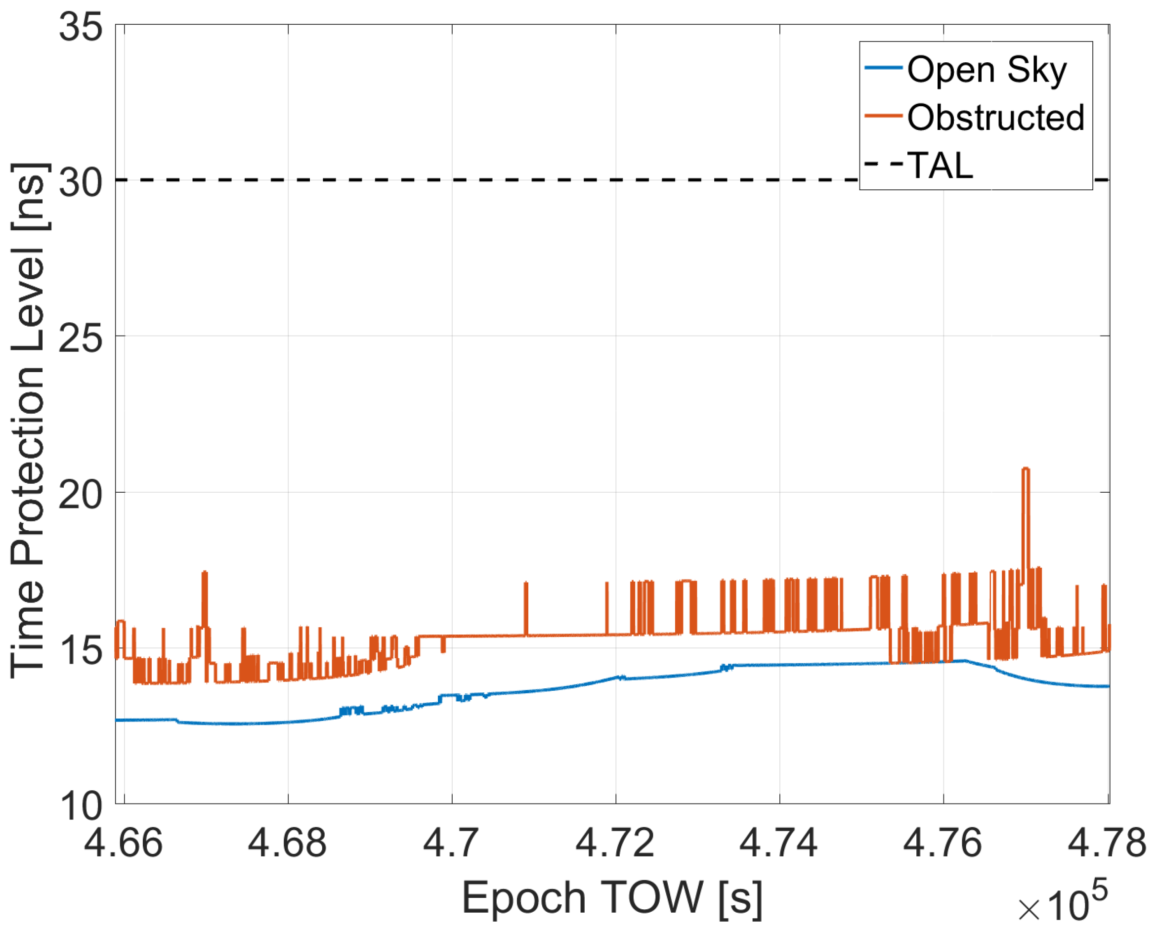
5. Results
6. Conclusions
- For averaging time interval smaller than 20 s, the Danish method provides the highest stability;
- For averaging time interval between 20 and 200 s the FB scheme is the one with the lowest ADEV values for the time-only solution case;
- For averaging time interval between 20 and 200 s for the full PVT solution the subset scheme provides the highest clock stability.
Funding
Data Availability Statement
Conflicts of Interest
References
- Bregni, S. Clock Stability Characterization and Measurement in Telecommunications. IEEE Trans. Instrum. Meas. 1997, 46, 1284–1294. [Google Scholar] [CrossRef]
- GSA. GNSS Market Report 2019; Technical Report; GSA: Prague, Czech Republic, 2019. [Google Scholar]
- EUSPA. EUSPA EO and GNSS Market Report 2022 Issue 1; Technical Report; EUSPA: Prague, Czech Republic, 2022. [Google Scholar]
- EU. Galileo Open Service—Service Definition Document; Technical Report Issue 1.2; European Union: Bruxelles, Belgium, 2021. [Google Scholar]
- EUSPA. Annex 4: Updates following the User Consultation Platform 2018: Report on Time & Synchronisation User Needs and Requirements; Technical Report; EU Agency for the Space Programme: Prague, Czech Republic, 2019. [Google Scholar]
- EUSPA. Report on Infrastructure User Needs and Requirements; Technical Report V1.0; EUSPA EU Agency for the Space Programme: Prague, Czech Republic, 2022. [Google Scholar]
- Catalano, V. EGNSS for Infrastructure. Presentation at the Euorpean Space Week 2022, Section on Critical Infrastructure. 2022. Available online: https://www.euspaceweek.eu/system/files/presentations/7-EGNSS%20For%20Infrastructure.pdf (accessed on 11 February 2023).
- Kaplan, E.D.; Hegarty, C. (Eds.) Understanding GPS: Principles and Applications, 2nd ed.; Artech House Publishers: Norwood, MA, USA, 2005. [Google Scholar]
- Kirkko-Jaakkola, M.; Thombre, S.; Honkala, S.; Soderholm, S.; Kaasalainen, S.; Kuusniemi, H.; Zelle, H.; Veerman, H.; Wallin, A.; Aarmo, K.; et al. Receiver-Level Robustness Concepts for EGNSS Timing Services. In Proceedings of the 30th International Technical Meeting of the Satellite Division of the Institute of Navigation (ION GNSS+ 2017), Portland, OR, USA, 25–29 September 2017. [Google Scholar]
- DEFIS. E.C. Directorate General for Defence Industry and Space Call for Tenders DEFIS/2021/OP/0004 Preparation of Standards for Galileo Timing Receivers. 2021. Available online: https://ted.europa.eu/udl?uri=TED:NOTICE:324819-2021:HTML:EN:HTML&tabId=1&tabLang=en (accessed on 11 February 2023).
- Geier, G.; King, T.; Kennedy, H.; Thomas, R.; McNamara, B. Prediction of the time accuracy and integrity of GPS timing. In Proceedings of the 1995 IEEE International Frequency Control Symposium (49th Annual Symposium), San Francisco, CA, USA, 31 May–2 June 1995. [Google Scholar] [CrossRef]
- Motorola. ONCORE Software Enanchements for Timing Applications; Technical Report; Motorola: San Diego, CA, USA, 1995. [Google Scholar]
- Gioia, C.; Borio, D. Multi-constellation T-RAIM: An experimental evaluation. In Proceedings of the 30th International Technical Meeting of The Satellite Division of the Institute of Navigation (ION GNSS+), Portlan, OR, USA, 25–29 September 2017. [Google Scholar]
- Gioia, C. GNSS Navigation in difficult environments: Hybridization and Reliability. Ph.D. Thesis, University Parthenope of Naples, Naples, Italy, 2014. [Google Scholar]
- Kuusniemi, H. User-Level Reliability and Quality Monitoring in Satellite-Based Personal Navigation. Ph.D. Thesis, Tampere University of Technology, Tampere, Finland, 2005. [Google Scholar]
- Hoffmann-Wellenhof, B.; Lichtenegger, H.; Collins, J. Global Positioning System: Theory and Practice; Springer: Berlin, Germany, 1992. [Google Scholar]
- Parkinson, B.; Spilker, J.; Axelrad, P.; Enge, P. Global Positioning System: Theory And Applications; American Institute of Aeronautics and Astronautics: Washington, DC, USA, 1996; Volume I. [Google Scholar]
- EU. European GNSS (Galileo) Open Service Signal-in-Space Interface Control Document; Technical Report Issue 1.2; European Union: Bruxelles, Belgium, 2016. [Google Scholar]
- Klobuchar, J.A. Ionospheric time-delay algorithm for single-frequency GPS usersIonospheric time-delay algorithm for single-frequency GPS users. IEEE Trans. Aerosp. Electron. Syst. 1987, 23, 325–331. [Google Scholar] [CrossRef]
- Sastamoinen, J. Contribution to The Theory of Atmospheric Refraction, Part II Refraction Correction in Satellite Geodesy. Bull. Geod. 1993, 107, 13–34. [Google Scholar] [CrossRef]
- Gioia, C.; Borio, D. A statistical characterization of the Galileo-to-GPS inter-system bias. J. Geod. 2016, 90, 1279–1291. [Google Scholar] [CrossRef]
- Petovello, M. Real-time Integration of a Tactical-Grade IMU and GPS for High-Accuracy Positioning and Navigation. Ph.D. Thesis, Department of Geomatics Engineering, University of Calgary, Calgary, AB, Canada, 2003. [Google Scholar]
- Angrisano, A.; Gaglione, S.; Gioia, C. Performance assessment of aided Global Navigation Satellite System for land navigation. IET Radar, Sonar Navig. 2013, 7, 671–680. [Google Scholar] [CrossRef]
- Borio, D.; Gioia, C. Galileo: The Added Value for Integrity in Harsh Environments. Sensors 2016, 16, 111. [Google Scholar] [CrossRef] [PubMed]
- Gioia, C.; Borio, D. Multi-Layer Defences for Robust GNSS Timing Retrieval. Sensors 2021, 21, 7787. [Google Scholar] [CrossRef] [PubMed]
- Walter, T.; Enge, P. Weighted RAIM for Precision Approach. In Proceedings of ION GPS; Institute of Navigation: Manassas, VA, USA, 1995. [Google Scholar]
- Ahmad, K.A.B. Reliability Monitoring of GNSS Aided Positioning for Land Vehicle Applications in Urban Environments. Ph.D. Thesis, Institut Superieur de lAeronautique et de lEspace, Toulouse, France, 2015. [Google Scholar]
- Baarda, W. A Testing Procedure for Use in Geodetic Networks; Publication on Geodesy New Series 2. No. 5; Netherlands Geodetic Commission: Delft, The Netherlands, 1968. [Google Scholar]
- Kuusniemi, H.; Wieser, A.; Lachapelle, G.; Takala, J. User-level reliability monitoring in urban personal satellite-navigation. IEEE Trans. Aerosp. Electron. Syst. 2007, 43, 1305–1318. [Google Scholar] [CrossRef]
- Angrisano, A.; Gaglione, S.; Gioia, C.; Del Core, G. GNSS Reliability Testing in Signal-Degraded Scenario. Int. J. Navig. Obs. 2013, 1, 1–12. [Google Scholar] [CrossRef]
- Lindsey, W.C.; Chie, C.M. Theory of oscillator instability based upon structure functions. Proc. IEEE 1976, 64, 1652–1666. [Google Scholar] [CrossRef]
- Allan, D. Statistics of atomic frequency standards. Proc. IEEE 1966, 54, 221–230. [Google Scholar] [CrossRef]
- Septentrio. Mosaic-X5 Product Datasheet. 2022. Available online: https://media.digikey.com/pdf/Data%20Sheets/Septentrio%20PDFs/Mosaic-X5_Datasheet.pdf (accessed on 11 February 2023).
- Cucchi, L.; Gioia, C.; Susi, M.; Damy, S.; Bonenberg, L.; Boniface, K.; Basso, M.; Sgammini, M.; Paonni, M.; Fortuny, J. JRC Testing and Demonstration Hub for the EU GNSS Programmes; Technical Report; Joint Reserach Centre: Ispra, Italy, 2021. [Google Scholar] [CrossRef]


| Scenario | Latitude [deg] | Longitude [deg] | Height [m] |
|---|---|---|---|
| Open-Sky | |||
| Obstructed |
| Scenario | Num Satellites | TTDOP | ||||
|---|---|---|---|---|---|---|
| Mean | Min | Max | Mean | Min | Max | |
| Open-Sky | 5 | 10 | ||||
| Obstructed | 2 | 6 | ||||
Disclaimer/Publisher’s Note: The statements, opinions and data contained in all publications are solely those of the individual author(s) and contributor(s) and not of MDPI and/or the editor(s). MDPI and/or the editor(s) disclaim responsibility for any injury to people or property resulting from any ideas, methods, instructions or products referred to in the content. |
© 2023 by the author. Licensee MDPI, Basel, Switzerland. This article is an open access article distributed under the terms and conditions of the Creative Commons Attribution (CC BY) license (https://creativecommons.org/licenses/by/4.0/).
Share and Cite
Gioia, C. T-RAIM Approaches: Testing with Galileo Measurements. Sensors 2023, 23, 2283. https://doi.org/10.3390/s23042283
Gioia C. T-RAIM Approaches: Testing with Galileo Measurements. Sensors. 2023; 23(4):2283. https://doi.org/10.3390/s23042283
Chicago/Turabian StyleGioia, Ciro. 2023. "T-RAIM Approaches: Testing with Galileo Measurements" Sensors 23, no. 4: 2283. https://doi.org/10.3390/s23042283
APA StyleGioia, C. (2023). T-RAIM Approaches: Testing with Galileo Measurements. Sensors, 23(4), 2283. https://doi.org/10.3390/s23042283