
sSLAM: Speeded-Up Visual SLAM Mixing Artificial Markers and Temporary Keypoints

 , ,
, ,  ,
,  and
and
Abstract
1. Introduction
2. Related Works
2.1. Visual SLAM
2.2. Fiducial Marker Systems
3. System Overview
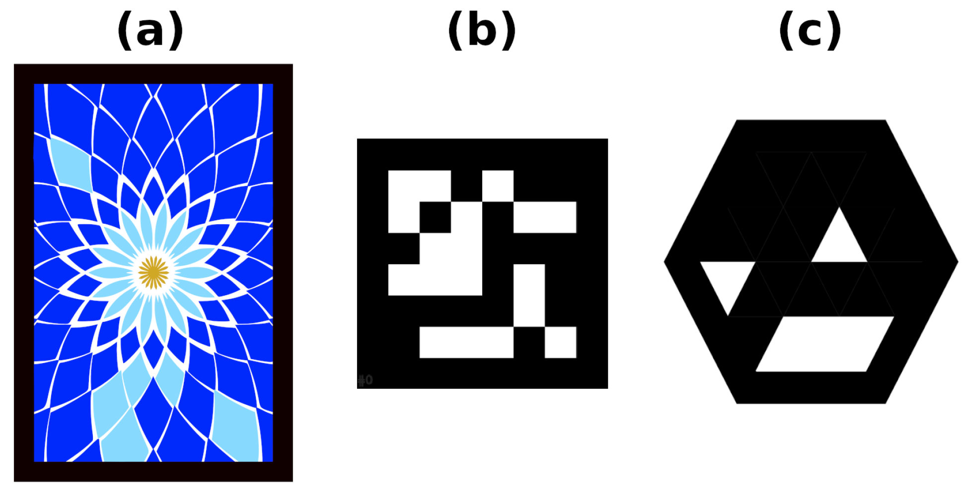
3.1. Markers
3.2. Frames
3.3. Keypoints
3.4. Map
3.5. Reprojection Error
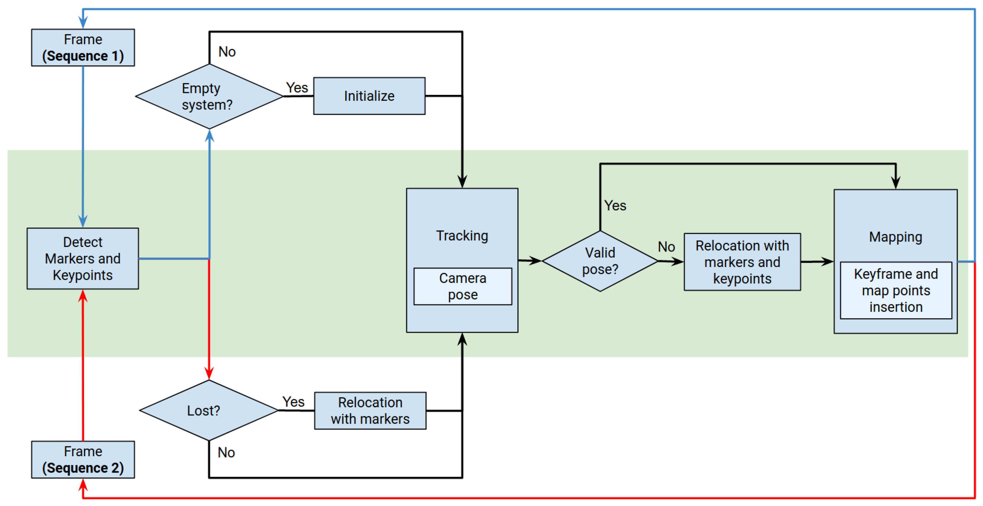
4. Proposed Method
4.1. Map Creation
4.2. Camera Localization
4.2.1. Relocalization with Markers
4.2.2. Tracking
4.2.3. Inserting and Removing Keyframes
5. Experiments and Results
5.1. Indoor Evaluation in Small Areas
5.2. Indoor Evaluation in Larger Areas
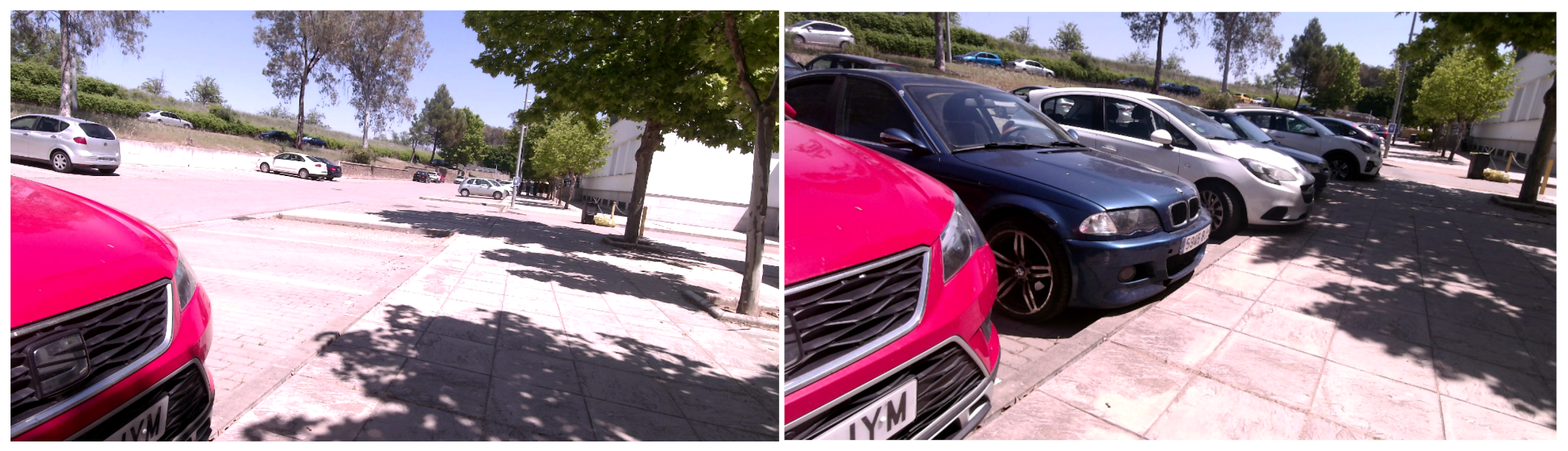
5.3. Outdoor Analysis
6. Conclusions and Future Work
Author Contributions
Funding
Data Availability Statement
Conflicts of Interest
References
- Taketomi, T.; Uchiyama, H.; Ikeda, S. Visual SLAM algorithms: A survey from 2010 to 2016. IPSJ Trans. Comput. Vis. Appl. 2017, 9, 16. [Google Scholar] [CrossRef]
- Morar, A.; Moldoveanu, A.; Mocanu, I.; Moldoveanu, F.; Radoi, I.E.; Asavei, V.; Gradinaru, A.; Butean, A. A Comprehensive Survey of Indoor Localization Methods Based on Computer Vision. Sensors 2020, 20, 2641. [Google Scholar] [CrossRef] [PubMed]
- Mur-Artal, R.; Tardós, J.D. ORB-SLAM2: An Open-Source SLAM System for Monocular, Stereo, and RGB-D Cameras. IEEE Trans. Robot. 2017, 33, 1255–1262. [Google Scholar] [CrossRef]
- Gao, X.; Wang, R.; Demmel, N.; Cremers, D. LDSO: Direct Sparse Odometry with Loop Closure. In Proceedings of the 2018 IEEE/RSJ International Conference on Intelligent Robots and Systems (IROS) 2018, Madrid, Spain, 1–5 October 2018; pp. 2198–2204. [Google Scholar]
- Campos, C.; Montiel, J.M.; Tardós, J.D. Fast and Robust Initialization for Visual-Inertial SLAM. In Proceedings of the 2019 International Conference on Robotics and Automation (ICRA), Montreal, QC, Canada, 20–24 May 2019; pp. 1288–1294. [Google Scholar]
- Munoz-Salinas, R.; Marin-Jimenez, M.J.; Medina-Carnicer, R. SPM-SLAM: Simultaneous localization and mapping with squared planar markers. Pattern Recognit. 2019, 86, 156–171. [Google Scholar] [CrossRef]
- Olson, E. AprilTag: A robust and flexible visual fiducial system. In Proceedings of the 2011 IEEE International Conference on Robotics and Automation, Shanghai, China, 9–13 May 2011; pp. 3400–3407. [Google Scholar]
- Romero-Ramirez, F.J.; Muñoz-Salinas, R.; Medina-Carnicer, R. Speeded Up Detection of Squared Fiducial Markers. Image Vis. Comput. 2018, 76, 38–47. [Google Scholar] [CrossRef]
- Muñoz-Salinas, R.; Medina-Carnicer, R. UcoSLAM: Simultaneous Localization and Mapping by Fusion of KeyPoints and Squared Planar Markers. Pattern Recognit. 2020, 101, 107193. [Google Scholar] [CrossRef]
- Campos, C.; Elvira, R.; Rodríguez, J.J.G.; Montiel, J.M.M.; Tardós, J.D. ORB-SLAM3: An Accurate Open-Source Library for Visual, Visual–Inertial, and Multimap SLAM. IEEE Trans. Robot. 2021, 37, 1874–1890. [Google Scholar] [CrossRef]
- Sumikura, S.; Shibuya, M.; Sakurada, K. OpenVSLAM: A Versatile Visual SLAM Framework. In Proceedings of the 27th ACM International Conference on Multimedia, MM ’19, Nice, France, 21–25 October 2019; ACM: New York, NY, USA, 2019; pp. 2292–2295. [Google Scholar]
- Davison, A.J.; Reid, I.D.; Molton, N.D.; Stasse, O. MonoSLAM: Real-Time Single Camera SLAM. IEEE Trans. Pattern Anal. Mach. Intell. 2007, 29, 1052–1067. [Google Scholar] [CrossRef] [PubMed]
- Eade, E.; Drummond, T. Scalable Monocular SLAM. In Proceedings of the 2006 IEEE Computer Society Conference on Computer Vision and Pattern Recognition (CVPR’06), New York, NY, USA, 17–22 June 2006; Volume 1, pp. 469–476. [Google Scholar]
- Eade, E.; Drummond, T. Edge landmarks in monocular SLAM. Image Vis. Comput. 2009, 27, 588–596. [Google Scholar] [CrossRef]
- Klein, G.; Murray, D. Parallel Tracking and Mapping for Small AR Workspaces. In Proceedings of the 2007 6th IEEE and ACM International Symposium on Mixed and Augmented Reality, Nara, Japan, 13–16 November 2007; pp. 225–234. [Google Scholar]
- Rosten, E.; Porter, R.; Drummond, T. Faster and Better: A Machine Learning Approach to Corner Detection. IEEE Trans. Pattern Anal. Mach. Intell. 2010, 32, 105–119. [Google Scholar] [CrossRef] [PubMed]
- Mur-Artal, R.; Montiel, J.M.M.; Tardós, J.D. ORB-SLAM: A Versatile and Accurate Monocular SLAM System. IEEE Trans. Robot. 2015, 31, 1147–1163. [Google Scholar] [CrossRef]
- Rublee, E.; Rabaud, V.; Konolige, K.; Bradski, G. ORB: An efficient alternative to SIFT or SURF. In Proceedings of the 2011 International Conference on Computer Vision, Barcelona, Spain, 6–13 November 2011; pp. 2564–2571. [Google Scholar]
- Garrido-Jurado, S.; Muñoz-Salinas, R.; Madrid-Cuevas, F.J.; Marín-Jiménez, M.J. Automatic generation and detection of highly reliable fiducial markers under occlusion. Pattern Recognit. 2014, 47, 2280–2292. [Google Scholar] [CrossRef]
- Fiala, M. Designing Highly Reliable Fiducial Markers. IEEE Trans. Pattern Anal. Mach. Intell. 2010, 32, 1317–1324. [Google Scholar] [CrossRef] [PubMed]
- Kato, H.; Billinghurst, M. Marker tracking and HMD calibration for a video-based augmented reality conferencing system. In Proceedings of the 2nd IEEE and ACM International Workshop on Augmented Reality (IWAR’99), San Francisco, CA, USA, 20–21 October 1999; pp. 85–94. [Google Scholar]
- Garrido-Jurado, S.; Garrido, J.; Jurado-Rodríguez, D.; Vázquez, F.; Muñoz-Salinas, R. Reflection-Aware Generation and Identification of Square Marker Dictionaries. Sensors 2022, 22, 8548. [Google Scholar] [CrossRef] [PubMed]
- Wagner, D.; Schmalstieg, D. ARToolKitPlus for Pose Tracking on Mobile Devices. In Proceedings of the Computer Vision Winter Workshop, St. Lambrecht, Austria, 6–8 February 2007; pp. 139–146. [Google Scholar]
- Jurado-Rodríguez, D.; Muñoz-Salinas, R.; Garrido-Jurado, S.; Medina-Carnicer, R. Design, Detection, and Tracking of Customized Fiducial Markers. IEEE Access 2021, 9, 140066–140078. [Google Scholar] [CrossRef]
- Collins, T.; Bartoli, A. Infinitesimal Plane-Based Pose Estimation. Int. J. Comput. Vis. 2014, 109, 252–286. [Google Scholar] [CrossRef]
- Ortiz-Fernandez, L.E.; Cabrera-Avila, E.V.; Silva, B.M.F.d.; Gonçalves, L.M.G. Smart Artificial Markers for Accurate Visual Mapping and Localization. Sensors 2021, 21, 625. [Google Scholar] [CrossRef] [PubMed]
- Peterson, W.W.; Brown, D.T. Cyclic Codes for Error Detection. Proc. IRE 1961, 49, 228–235. [Google Scholar] [CrossRef]
- Galvez-López, D.; Tardos, J.D. Bags of Binary Words for Fast Place Recognition in Image Sequences. IEEE Trans. Robot. 2012, 28, 1188–1197. [Google Scholar] [CrossRef]
- Horn, B.K.P. Closed-form solution of absolute orientation using unit quaternions. J. Opt. Soc. Am. A 1987, 4, 629–642. [Google Scholar] [CrossRef]


| Experiment | Zone | Video (#Frames) |
|---|---|---|
| Indoor room | Ceilings | video-01 (3106) |
| video-02 (2603) | ||
| video-03 (2403) | ||
| Walls | video-04 (1682) | |
| video-05 (2889) | ||
| video-06 (3458) | ||
| Large indoor | Corridor | video-07 (16,838) |
| video-08 (17,420) | ||
| Outdoor | Zone-0 | video-09 (7456) |
| video-10 (8361) | ||
| video-11 (6885) | ||
| video-12 (6329) | ||
| video-13 (6885) | ||
| Zone-1 | video-14 (1888) | |
| video-15 (1710) | ||
| video-16 (1891) | ||
| Zone-2 | video-17 (6190) | |
| video-18 (4922) | ||
| Zone-3 | video-19 (5335) | |
| video-20 (5453) | ||
| video-21 (5177) | ||
| video-22 (5191) |
| Parameter | Value | Description |
|---|---|---|
| Subsampling scale factor (Section 3.2) | ||
| 7 | Maximum level of the pyramid (Section 3.3) | |
| [10…120] | Maximum number of keyframes (Section 3.4) | |
| Minimum weight of markers. (Section 3.5) | ||
| Percentage of minimum image area occupied by markers. (Section 3.5) | ||
| 30 | Minimum matches required (Section 4.2.1) | |
| Threshold for adding new keyframes (Section 4.2.3) |
| Indoor | Outdoor | ||
|---|---|---|---|
| OpenVSLAM | ATE | N (, ) | N (, ) |
| pTrck | Y (, ) | N (, ) | |
| FPS | Y (, ) | Y (, ) | |
| ORB-SLAM2 | ATE | N (, ) | N (, ) |
| pTrck | N (, ) | N (, ) | |
| FPS | Y (, ) | Y (, ) | |
| ORB-SLAM3 | ATE | Y (, ) | N (, ) |
| pTrck | N (, ) | N (, ) | |
| FPS | Y (, | Y (, ) | |
| UcoSLAM | ATE | N (, ) | N (, ) |
| pTrck | Y (, ) | Y (, ) | |
| FPS | Y (, ) | Y (, ) |
Disclaimer/Publisher’s Note: The statements, opinions and data contained in all publications are solely those of the individual author(s) and contributor(s) and not of MDPI and/or the editor(s). MDPI and/or the editor(s) disclaim responsibility for any injury to people or property resulting from any ideas, methods, instructions or products referred to in the content. |
© 2023 by the authors. Licensee MDPI, Basel, Switzerland. This article is an open access article distributed under the terms and conditions of the Creative Commons Attribution (CC BY) license (https://creativecommons.org/licenses/by/4.0/).
Share and Cite
Romero-Ramirez, F.J.; Muñoz-Salinas, R.; Marín-Jiménez, M.J.; Cazorla, M.; Medina-Carnicer, R. sSLAM: Speeded-Up Visual SLAM Mixing Artificial Markers and Temporary Keypoints. Sensors 2023, 23, 2210. https://doi.org/10.3390/s23042210
Romero-Ramirez FJ, Muñoz-Salinas R, Marín-Jiménez MJ, Cazorla M, Medina-Carnicer R. sSLAM: Speeded-Up Visual SLAM Mixing Artificial Markers and Temporary Keypoints. Sensors. 2023; 23(4):2210. https://doi.org/10.3390/s23042210
Chicago/Turabian StyleRomero-Ramirez, Francisco J., Rafael Muñoz-Salinas, Manuel J. Marín-Jiménez, Miguel Cazorla, and Rafael Medina-Carnicer. 2023. "sSLAM: Speeded-Up Visual SLAM Mixing Artificial Markers and Temporary Keypoints" Sensors 23, no. 4: 2210. https://doi.org/10.3390/s23042210
APA StyleRomero-Ramirez, F. J., Muñoz-Salinas, R., Marín-Jiménez, M. J., Cazorla, M., & Medina-Carnicer, R. (2023). sSLAM: Speeded-Up Visual SLAM Mixing Artificial Markers and Temporary Keypoints. Sensors, 23(4), 2210. https://doi.org/10.3390/s23042210