

Position and Attitude Determination in Urban Canyon with Tightly Coupled Sensor Fusion and a Prediction-Based GNSS Cycle Slip Detection Using Low-Cost Instruments


Abstract
:1. Introduction
2. Sensor Models
2.1. GNSS Receivers
2.2. Inertial, Magnetic and Barometric Sensors
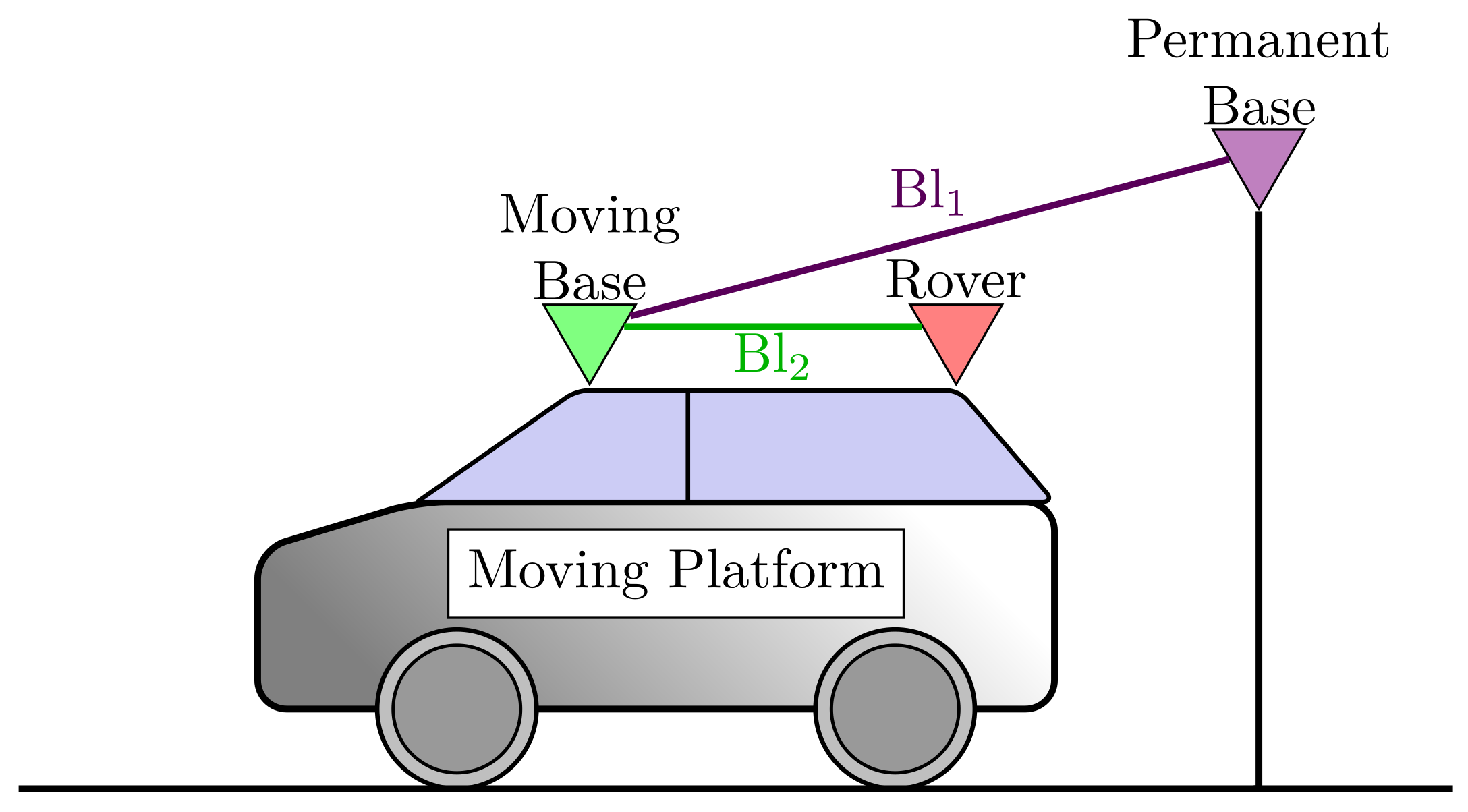
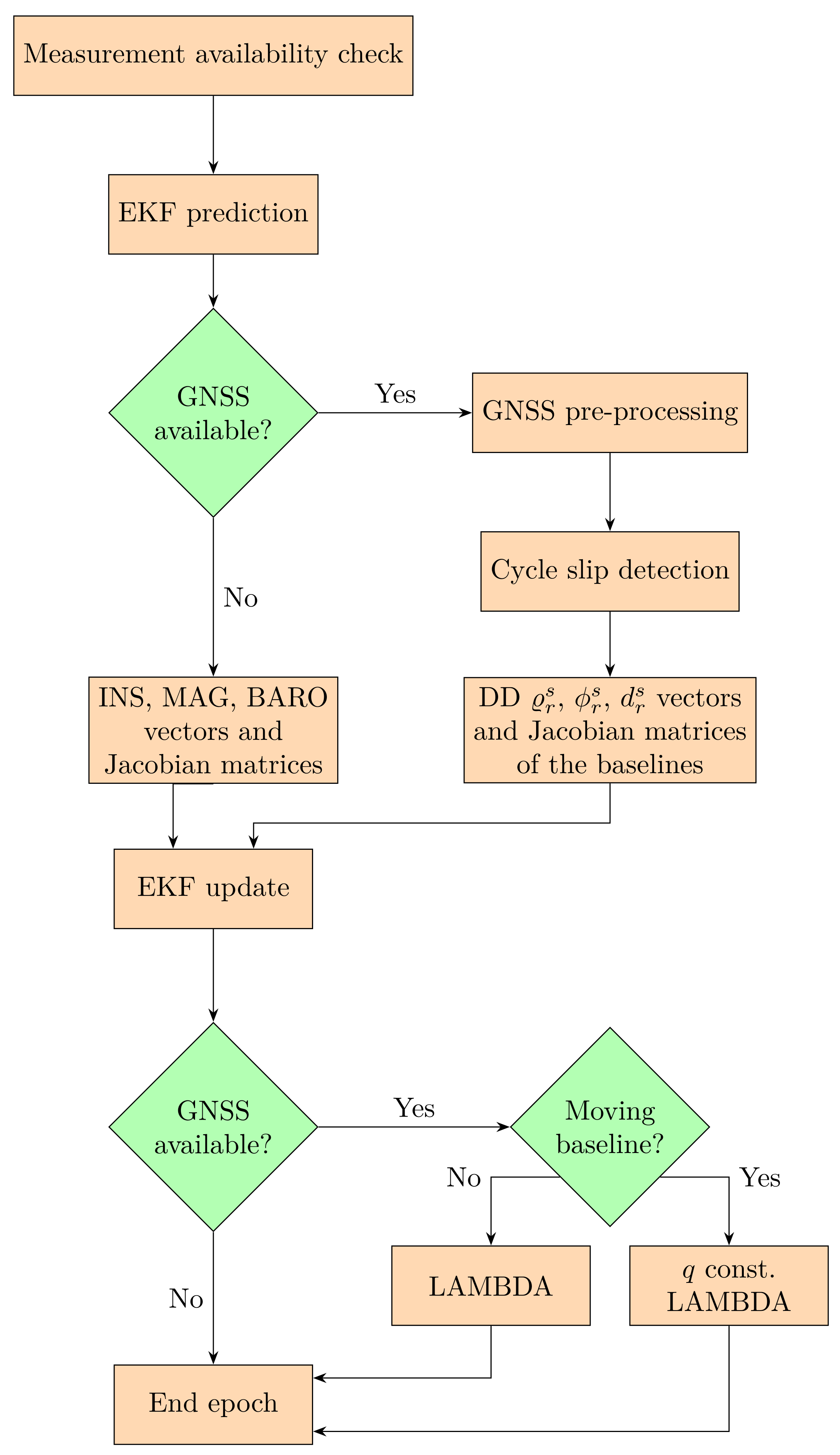
3. The Estimation Algorithm
- Position (), velocity () and acceleration () of the Moving Base antenna in Earth-Centered Earth-Fixed (ECEF) Coordinate system;
- Orientation quaternions (), angular velocities ();
- Accelerometer bias error (), gyroscope bias error (), magnetometer bias error (), barometer bias error ();
- Local magnetic field ();
- GNSS receiver clock biases for every receiver ();
- GNSS receiver clock drifts for every receiver ();
- Single-differenced GLONASS system related receiver inter-channel biases for every baseline ();
- Single-differenced integer ambiguities for every baseline and every satellite ().
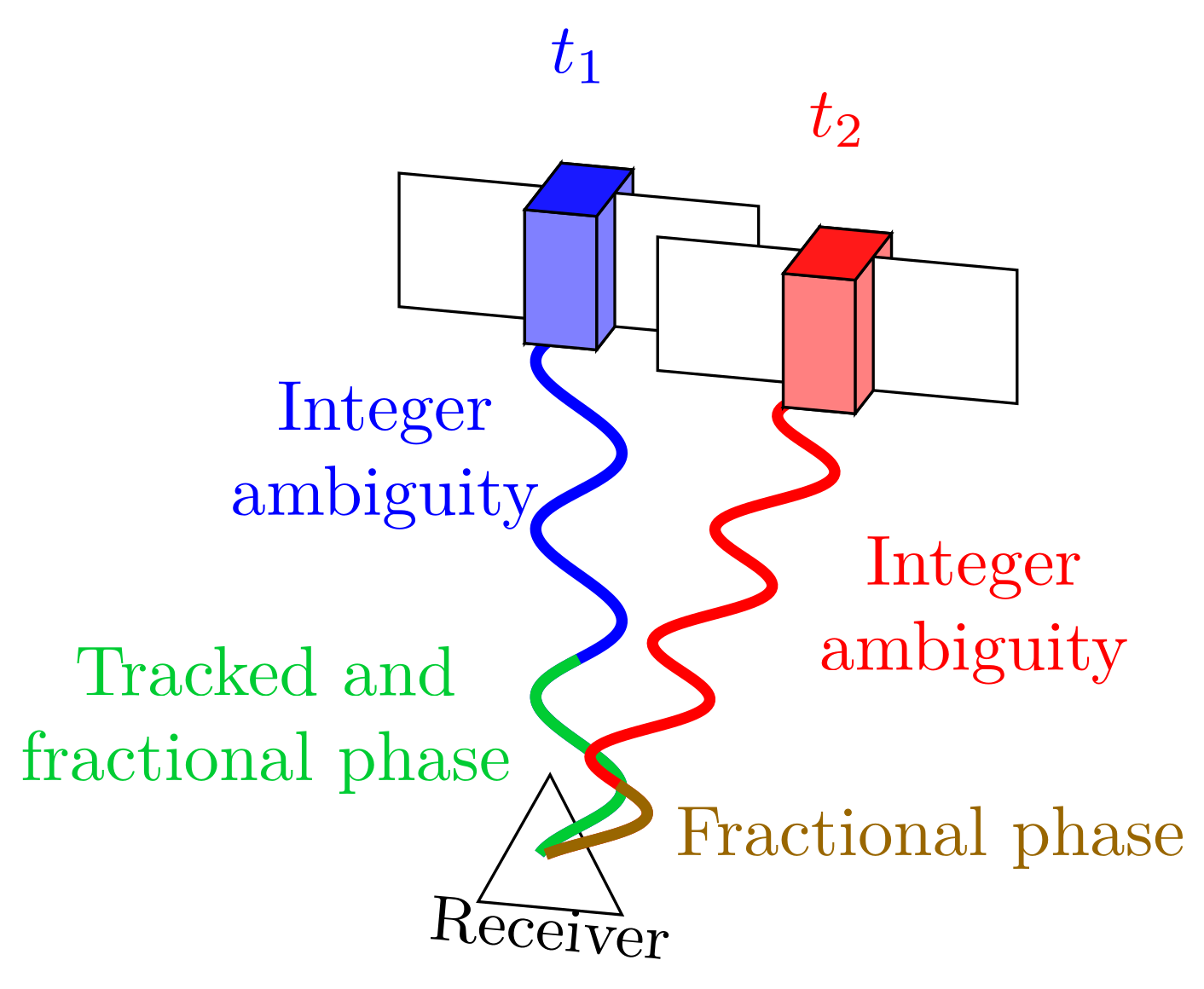
4. Cycle Slip Detection Techniques for Moving Platforms
4.1. Loss-of-Lock Indicator-Based Cycle Slip Detection
4.2. Cycle Slip Detection Using the Melbourne–Wübbena Linear Combination
4.3. The TurboEdit Cycle Slip Detection Method
4.4. The Prediction-Based Cycle Slip Detection Algorithm
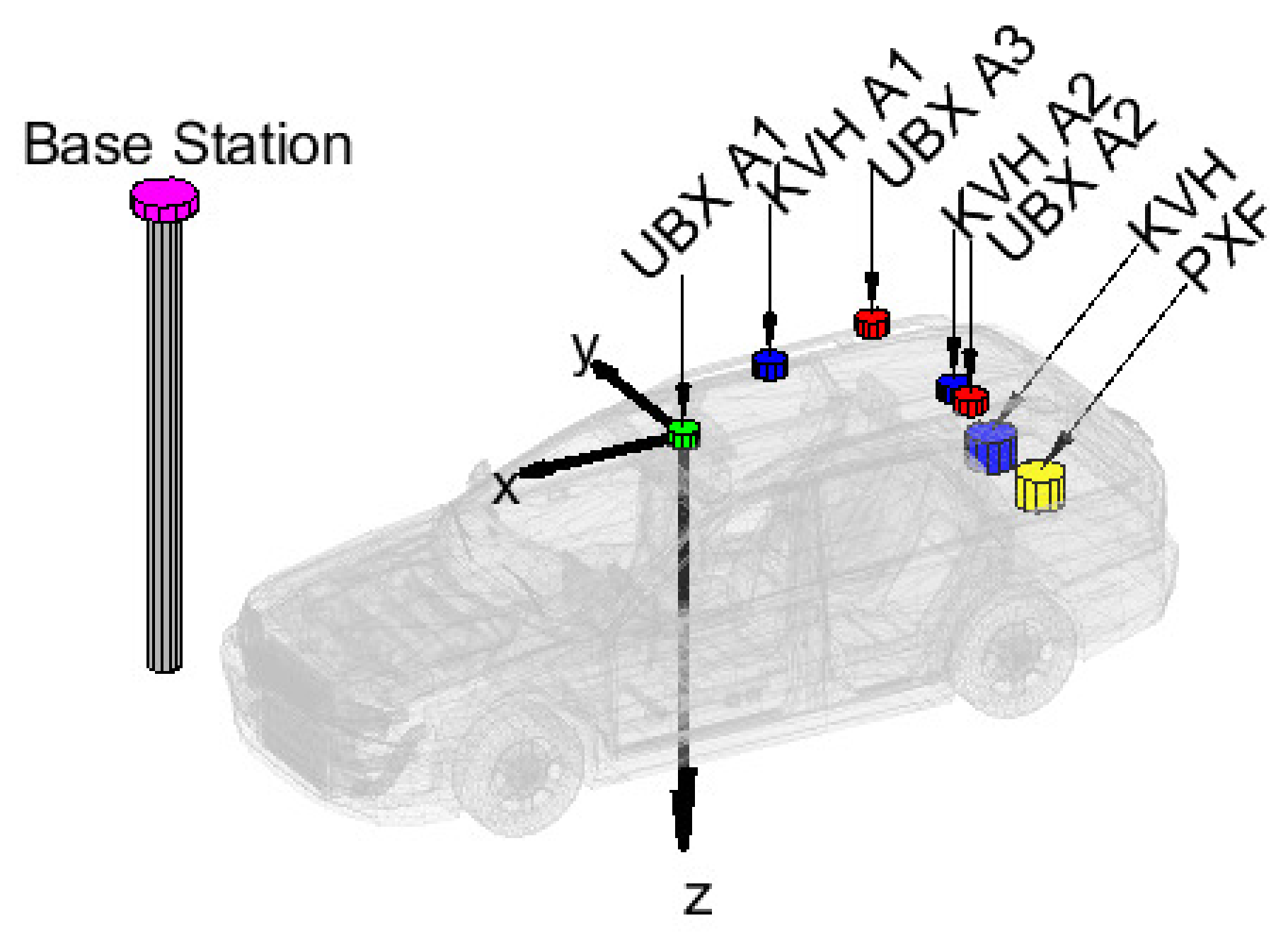
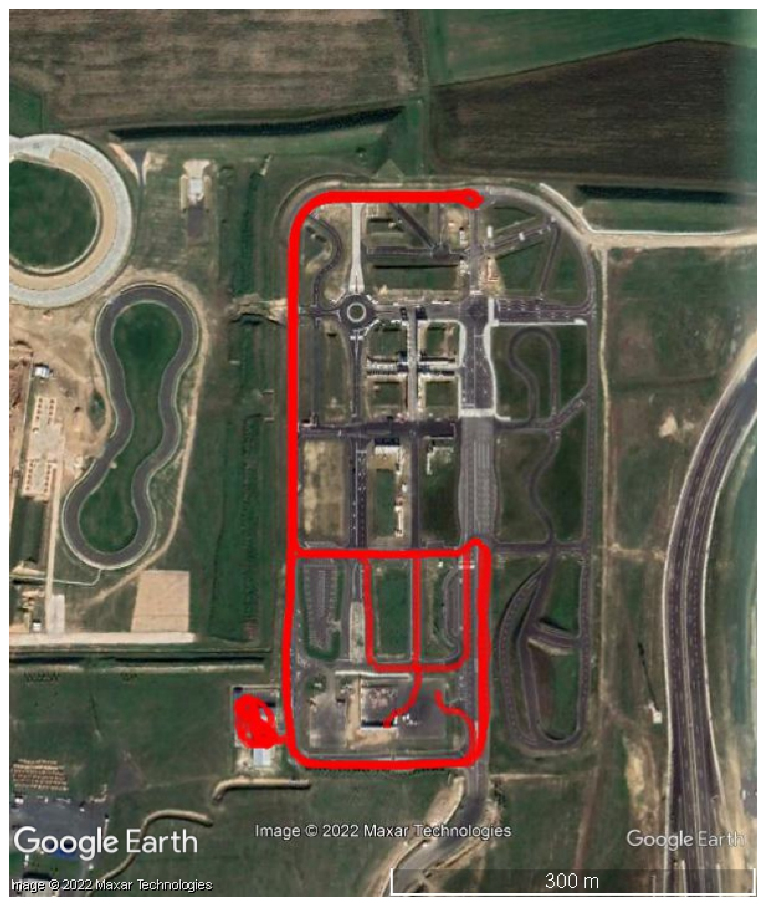
5. Measurement Platform
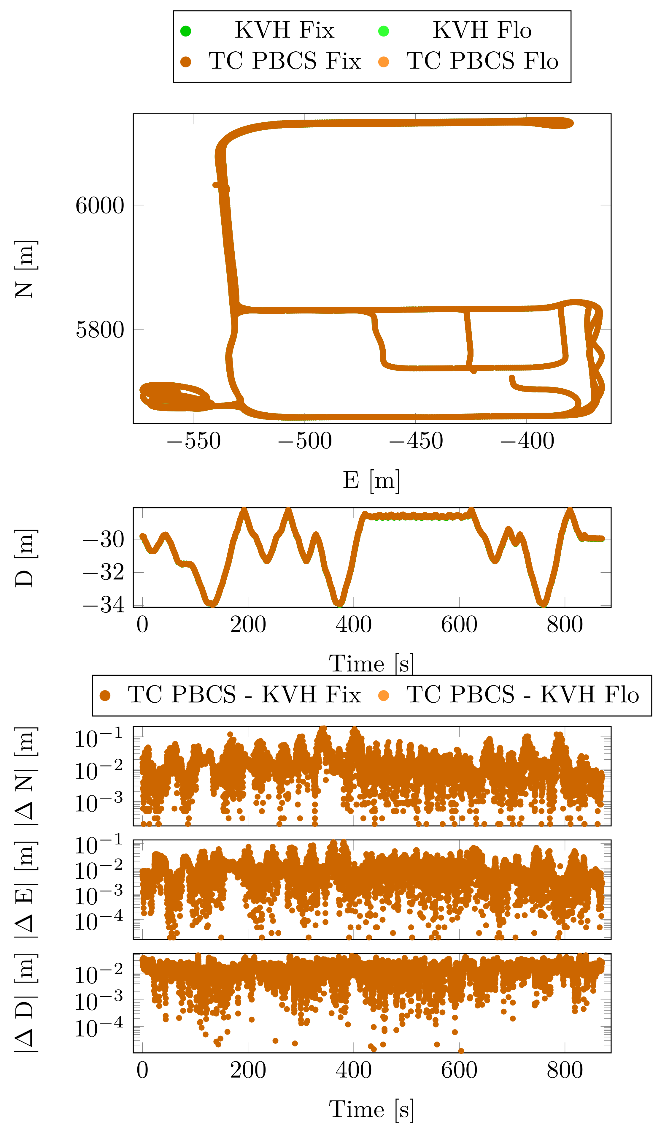
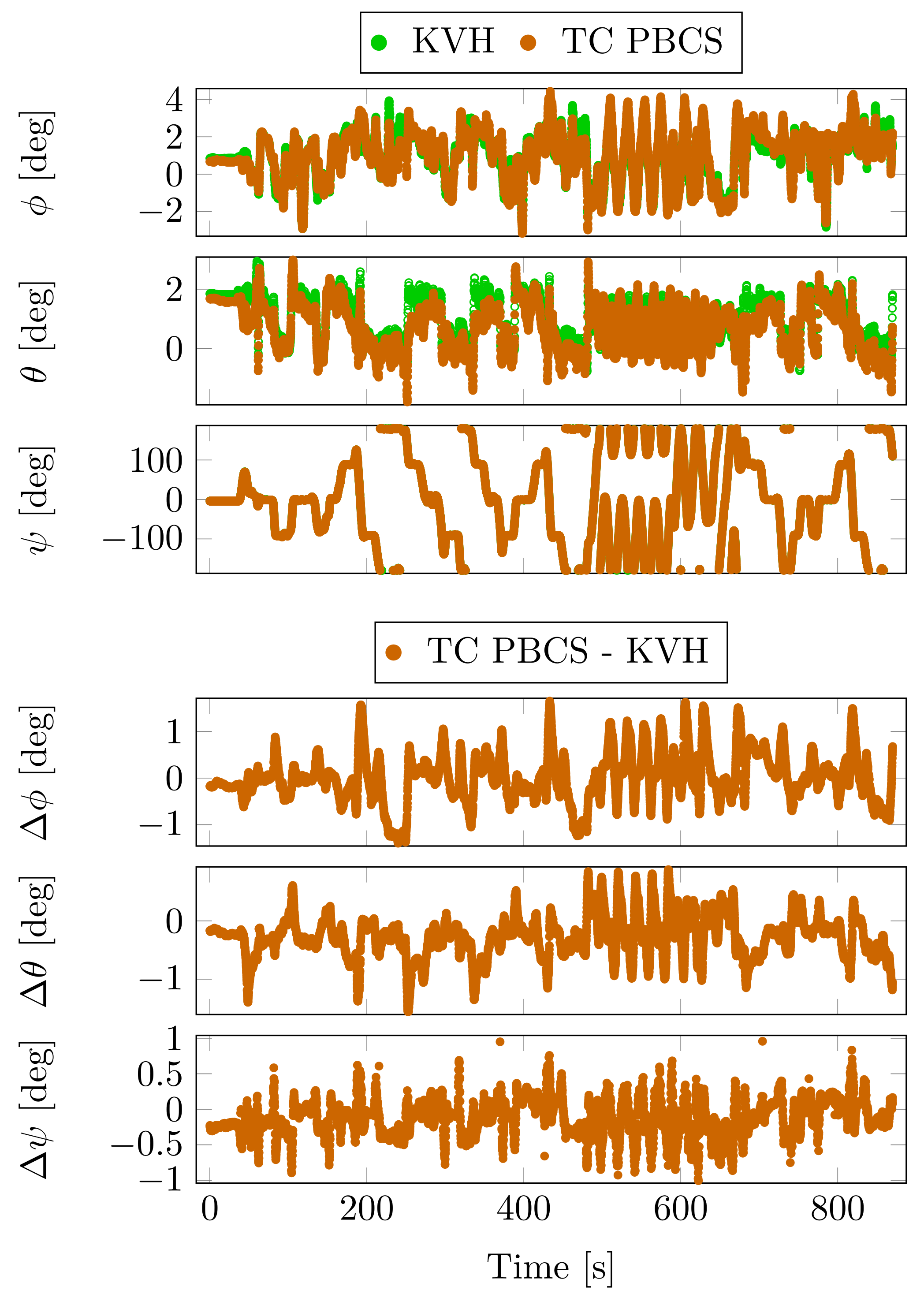
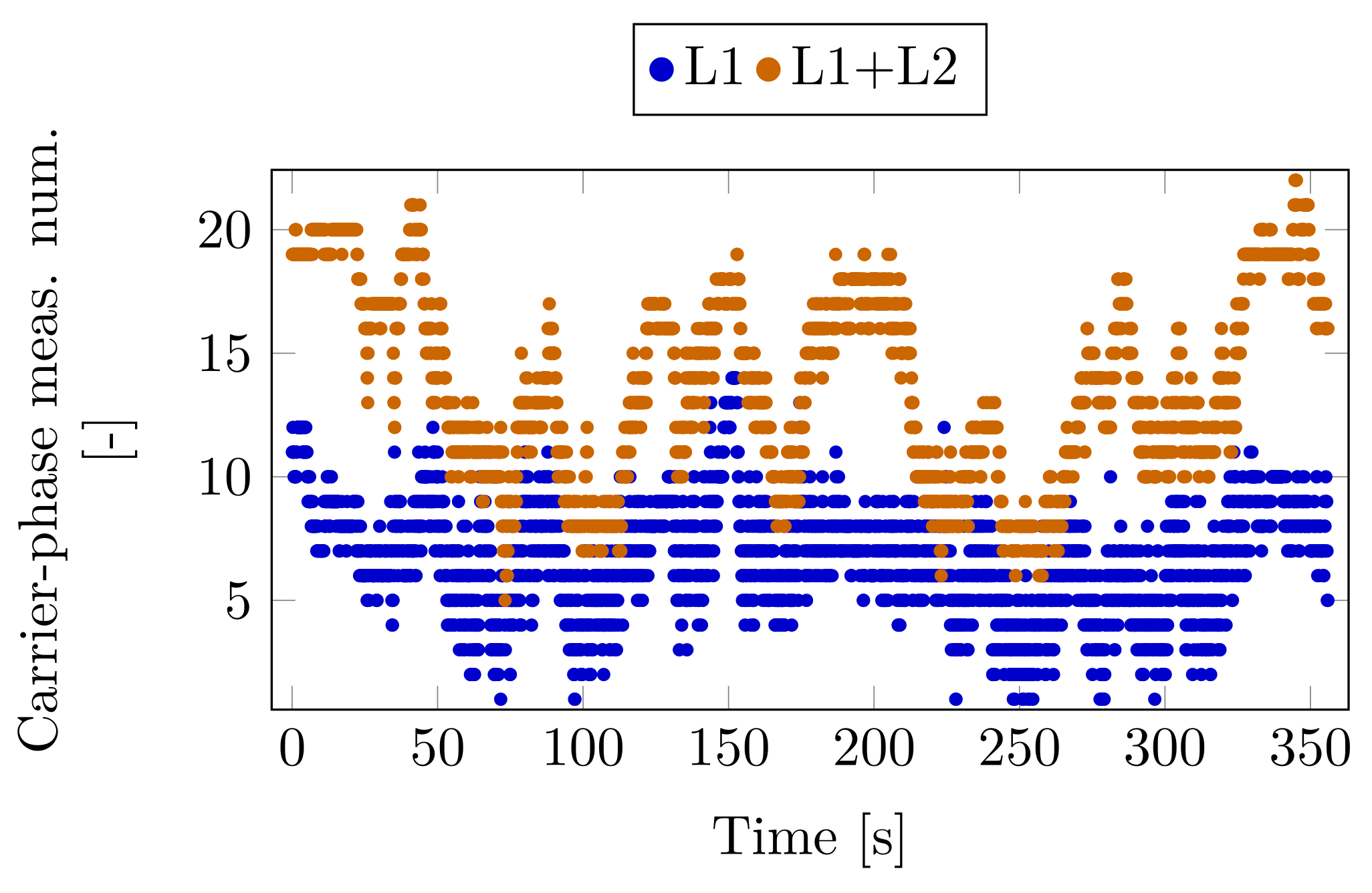
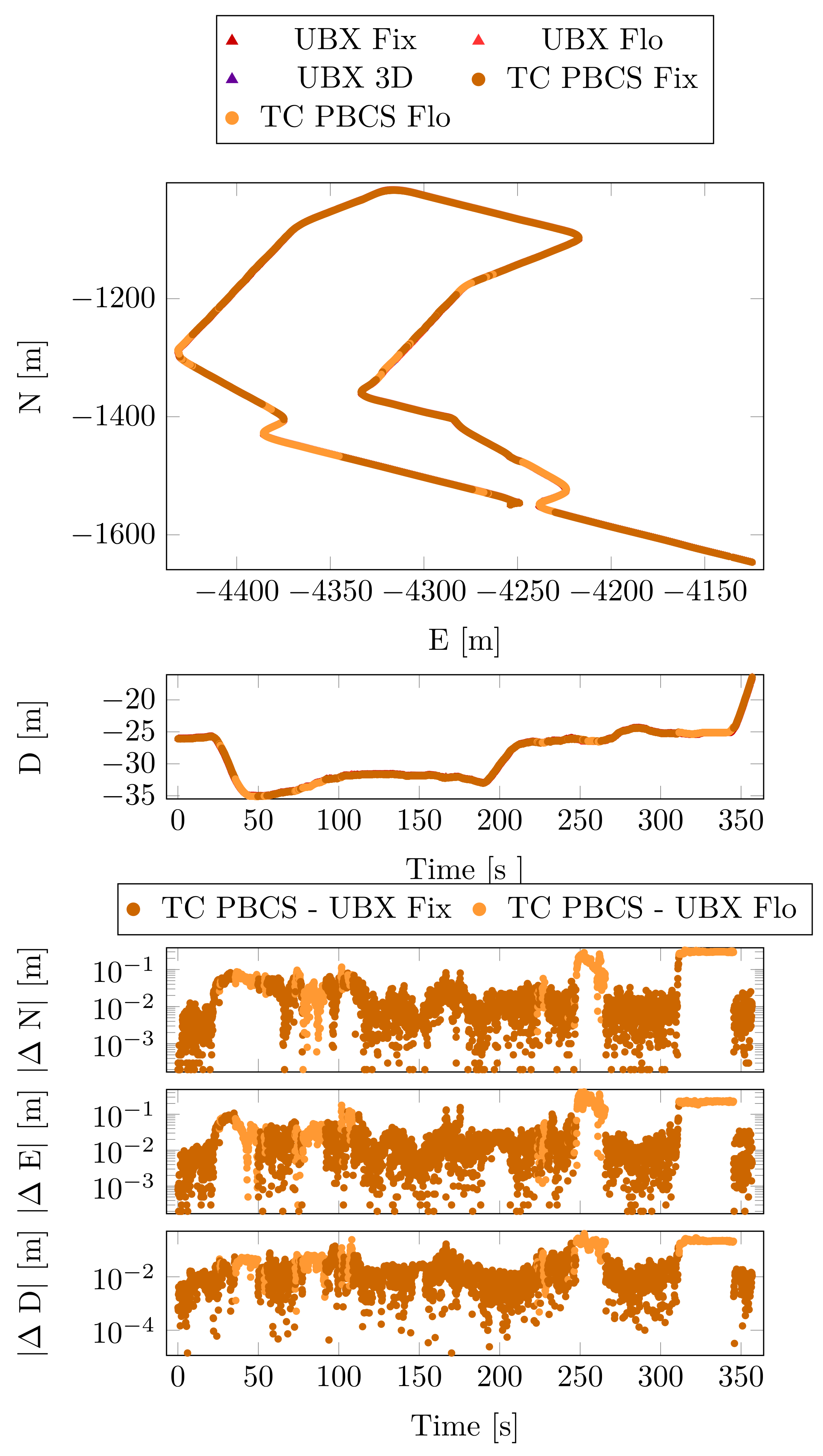
6. Case Study 1
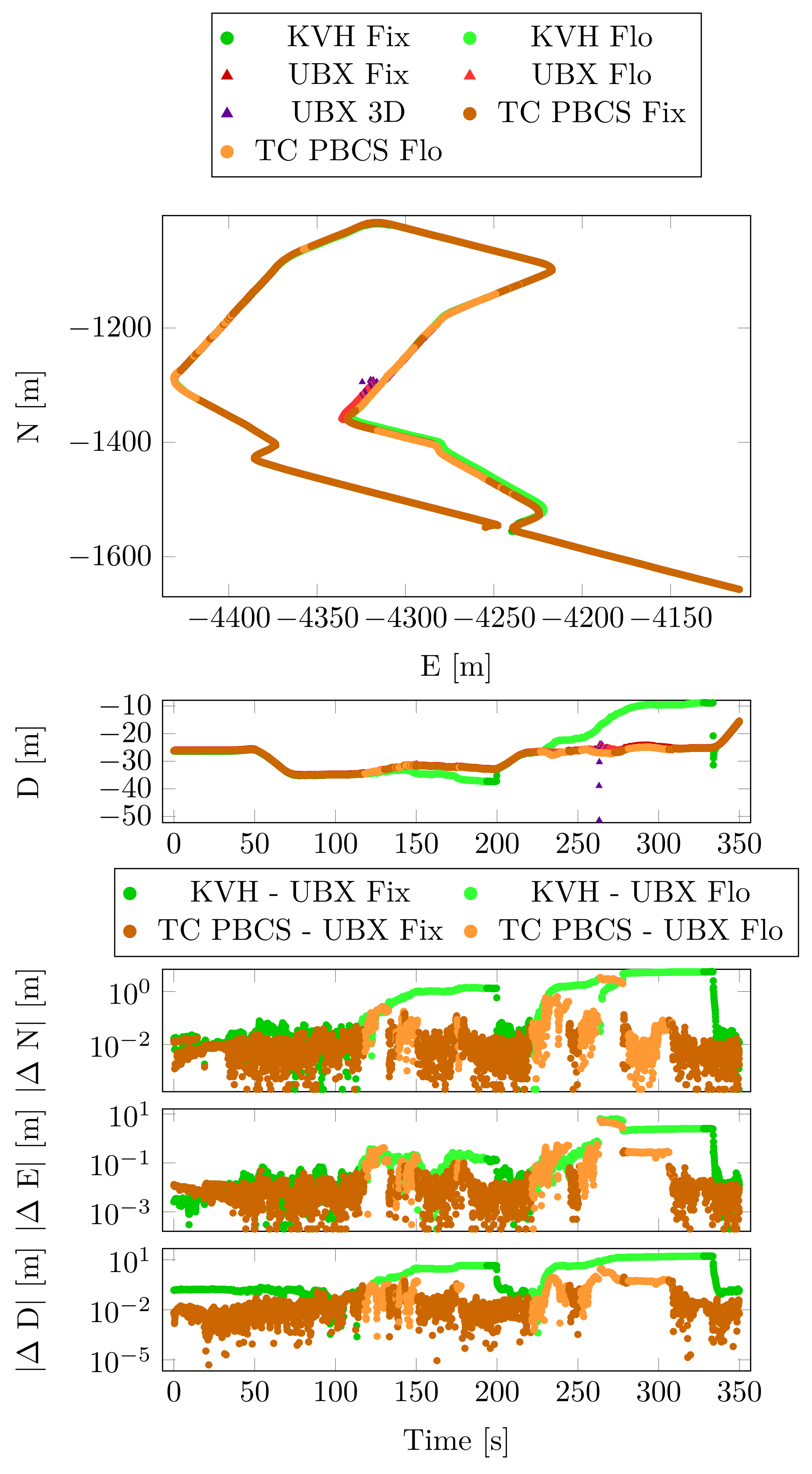
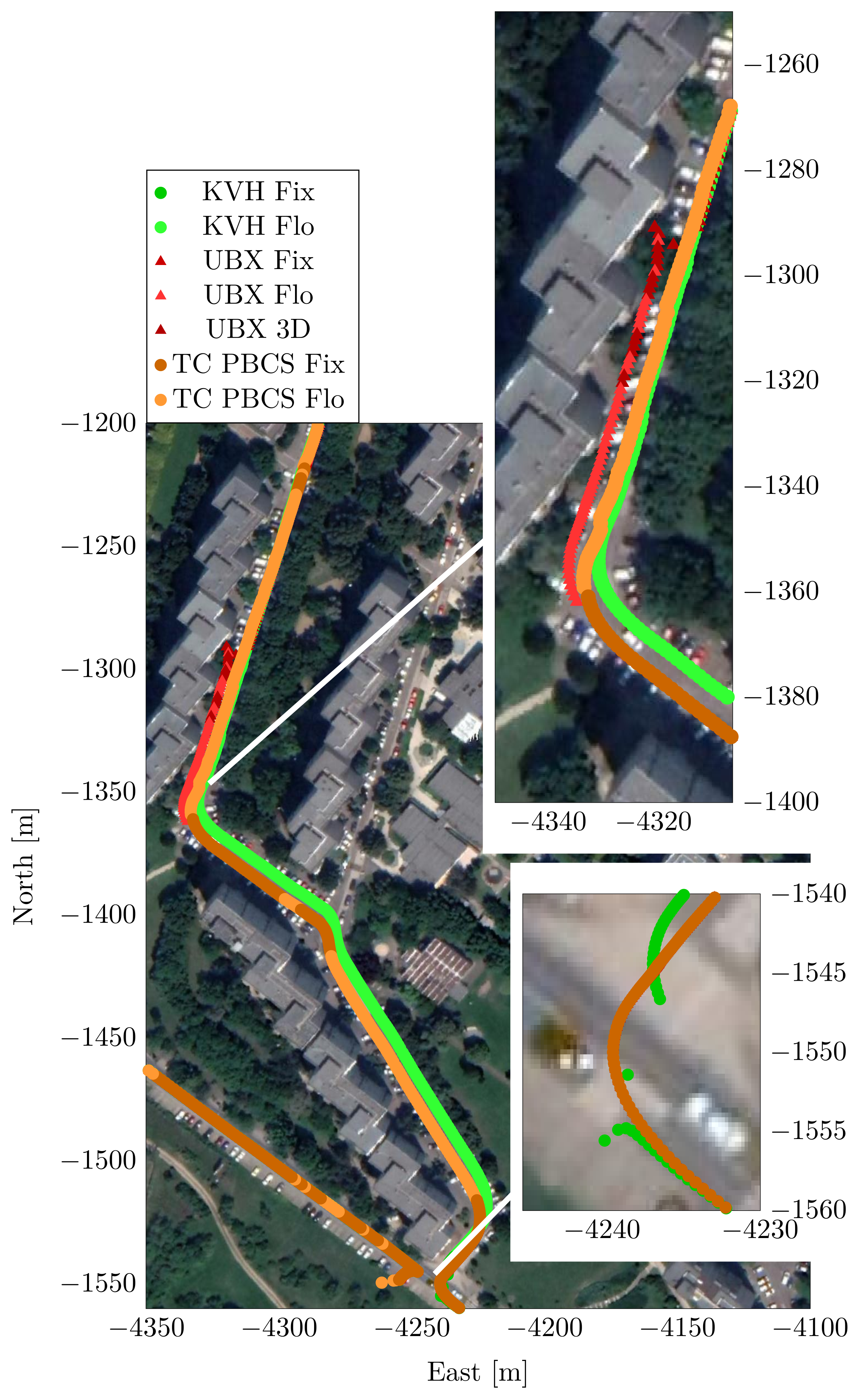
7. Case Study 2
8. Case Study 3
9. Discussion
Author Contributions
Funding
Data Availability Statement
Conflicts of Interest
Abbreviations
| TC | Tightly Coupled Sensor Integration |
| LLI | Loss-of-Lock Indicator |
| PBCS | Prediction-Based Cycle Slip |
| MW | Melbourne–Wübbena method |
| TE | TurboEdit method |
| SD | Single Difference |
| DD | Double Difference |
| TD | Triple Difference |
References
- Groves, P.D. Principles of GNSS, Inertial, and Multisensor Integrated Navigation Systems, 2nd ed.; Artech House: Norwood, MA, USA, 2013. [Google Scholar]
- Lipp, A.; Gu, X. Cycle-slip detection and repair in integrated navigation systems. In Proceedings of the 1994 IEEE Position, Location and Navigation Symposium-PLANS’94, Las Vegas, NV, USA, 11–15 April 1994; IEEE: Piscataway Township, NJ, USA, 1994; pp. 681–688. [Google Scholar]
- Melbourne, W. The case for ranging in GPS-based geodetic systems. In Proceedings of the 1st International Symposium on Precise Positioning with GPS, Rockville, MD, USA, 15–19 April 1985; pp. 373–386. [Google Scholar]
- Wubbena, G. Software developments for geodetic positioning with GPS using TI 4100 code and carrier measurements. In Proceedings of the 1st International Symposium on Precise Positioning with the Global Positioning System, Rockville, MD, USA, 15–19 April 1985; US Department of Commerce: Washington, DC, USA, 1985; pp. 403–412. [Google Scholar]
- Blewitt, G. An automatic editing algorithm for GPS data. Geophys. Res. Lett. 1990, 17, 199–202. [Google Scholar] [CrossRef]
- Xu, X.; Nie, Z.; Wang, Z.; Zhang, Y. A Modified TurboEdit Cycle-Slip Detection and Correction Method for Dual-Frequency Smartphone GNSS Observation. Sensors 2020, 20, 5756. [Google Scholar] [CrossRef] [PubMed]
- de Lacy, M.C.; Reguzzoni, M.; Sanso, F. Real-time cycle slip detection in triple-frequency GNSS. GPS Solut. 2012, 16, 353–362. [Google Scholar] [CrossRef]
- Lee, H.K.; Wang, J.; Rizos, C. Effective cycle slip detection and identification for high precision GPS/INS integrated systems. J. Navig. 2003, 56, 475–486. [Google Scholar] [CrossRef]
- Yoon, Y.M.; Lee, B.S.; Heo, M.B. Multiple Cycle Slip Detection Algorithm for a Single Frequency Receiver. Sensors 2022, 22, 2525. [Google Scholar] [CrossRef] [PubMed]
- Kim, Y.; Song, J.; Kee, C.; Park, B. GPS cycle slip detection considering satellite geometry based on TDCP/INS integrated navigation. Sensors 2015, 15, 25336–25365. [Google Scholar] [CrossRef] [PubMed]
- Kim, J.; Kim, Y.; Song, J.; Kim, D.; Park, M.; Kee, C. Performance improvement of time-differenced carrier phase measurement-based integrated GPS/INS considering noise correlation. Sensors 2019, 19, 3084. [Google Scholar] [CrossRef] [PubMed]
- Kim, J.; Park, M.; Bae, Y.; Kim, O.J.; Kim, D.; Kim, B.; Kee, C. A low-cost, high-precision vehicle navigation system for deep urban multipath environment using TDCP measurements. Sensors 2020, 20, 3254. [Google Scholar] [CrossRef] [PubMed]
- Hofmann-Wellenhof, B.; Lichtenegger, H.; Collins, J. Global Positioning System: Theory and Practice; Springer Science & Business Media: Berlin/Heidelberg, Germany, 2012. [Google Scholar]
- Henkel, P.; Iafrancesco, M. Tightly coupled position and attitude determination with two low-cost GNSS receivers. In Proceedings of the Wireless Communications Systems (ISWCS), 2014 11th International Symposium on IEEE, Barcelona, Spain, 26–29 August 2014; pp. 895–900. [Google Scholar]
- National Oceanic, Atmospheric Administration; United States Air Force. US Standard Atmosphere, 1976; National Oceanic and Atmospheric Administration: Washington, DC, USA, 1976; Volume 76. [Google Scholar]
- Farkas, M.; Vanek, B.; Rozsa, S. Small UAV’s position and attitude estimation using tightly coupled multi baseline multi constellation GNSS and inertial sensor fusion. In Proceedings of the 2019 IEEE 5th International Workshop on Metrology for AeroSpace (MetroAeroSpace), Torino, Italy, 19–21 June 2019; pp. 176–181. [Google Scholar] [CrossRef]
- Bishop, G.; Welch, G. An introduction to the Kalman filter. Proc. Siggraph Course 2001, 8, 59. [Google Scholar]
- Teunissen, P.J. The least-squares ambiguity decorrelation adjustment: A method for fast GPS integer ambiguity estimation. J. Geod. 1995, 70, 65–82. [Google Scholar] [CrossRef]
- Teunissen, P.J. The LAMBDA method for the GNSS compass. Artif. Satell. 2006, 41, 89–103. [Google Scholar] [CrossRef]
- Giorgi, G. GNSS Carrier Phase-Based Attitude Determination Estimation and Applications; Delft University of Technology: Delft, The Netherlands, 2011. [Google Scholar]
- Giorgi, G.; Teunissen, P.J. Carrier phase GNSS attitude determination with the multivariate constrained LAMBDA method. In Proceedings of the Aerospace Conference, Big Sky, MO, USA, 6–13 March 2010; IEEE: Piscataway Township, NJ, USA, 2010; pp. 1–12. [Google Scholar]
- Wang, B.; Miao, L.; Wang, S.; Shen, J. A constrained LAMBDA method for GPS attitude determination. GPS Solut. 2009, 13, 97–107. [Google Scholar] [CrossRef]
- Dach, R.; Lutz, S.; Walser, P.; Fridez, P. Bernese GNSS Software Version 5.2. 2015. Available online: http://www.bernese.unibe.ch/ (accessed on 29 January 2023).
- Henkel, P.; Oku, N. Cycle slip detection and correction for heading determination with low-cost GPS/INS receivers. In Proceedings of the VIII Hotine-Marussi Symposium on Mathematical Geodesy: Symposium in Rome, Rome, Italy, 17–21 June 2013; Springer: Berlin/Heidelberg, Germany, 2016; pp. 291–299. [Google Scholar]
- Szalay, Z.; Hamar, Z.; Nyerges, Á. Novel design concept for an automotive proving ground supporting multilevel CAV development. Int. J. Veh. Des. 2019, 80, 1–22. [Google Scholar] [CrossRef]
- Takasu, T. Technology Evolution of Multi-Constellation RTK. Available online: https://gpspp.sakura.ne.jp/paper2005/IPNTJ_NEXTWG_202102.pdf (accessed on 29 January 2023).


| UBX A1 | UBX A2 | UBX A3 | PXF | KVH | KVH A1 | KVH A2 | |
|---|---|---|---|---|---|---|---|
| x [m] | 0.00 | −0.98 | −0.98 | −1.80 | −1.80 | −0.40 | −0.98 |
| y [m] | 0.00 | −0.45 | 0.45 | 0.00 | 0.29 | 0.37 | −0.26 |
| z [m] | 0.00 | −0.08 | −0.08 | 0.90 | 0.90 | −0.03 | −0.03 |
| PBCS | LLI | MW | TE | UBX | KVX | |
|---|---|---|---|---|---|---|
| Bl1 AR [%] | 100.00 | 99.19 | 99.20 | 99.87 | 88.80 | 100.0 |
| Bl2 AR [%] | 100.00 | 100.00 | 100.00 | 96.77 | - | - |
| Bl3 AR [%] | 100.00 | 100.00 | 100.00 | 96.77 | - | - |
| NPBCS | NLLI | NMW | NTE | NUBX | |
| Fix. Mean [m] | 0.01 | 0.01 | 0.01 | 0.01 | 0.00 |
| Fix. Std. [m] | 0.02 | 0.02 | 0.02 | 0.02 | 0.01 |
| Fix. Max(abs) [m] | 0.18 | 0.20 | 0.20 | 0.25 | 0.08 |
| Flo. Mean [m] | 0.00 | −0.50 | −0.52 | 0.07 | 0.03 |
| Flo. Std. [m] | 0.00 | 0.02 | 0.02 | 0.01 | 0.25 |
| Flo. Max(abs) [m] | 0.00 | 0.53 | 0.54 | 0.09 | 0.67 |
| EPBCS | ELLI | EMW | ETE | EUBX | |
| Fix. Mean [m] | 0.01 | 0.01 | 0.01 | 0.01 | 0.01 |
| Fix. Std. [m] | 0.01 | 0.01 | 0.01 | 0.01 | 0.01 |
| Fix. Max(abs) [m] | 0.11 | 0.11 | 0.11 | 0.22 | 0.05 |
| Flo. Mean [m] | 0.00 | 0.42 | 0.43 | 0.12 | 0.15 |
| Flo. Std. [m] | 0.00 | 0.01 | 0.01 | 0.08 | 0.11 |
| Flo. Max(abs) [m] | 0.00 | 0.44 | 0.45 | 0.22 | 0.41 |
| DPBCS | DLLI | DMW | DTE | DUBX | |
| Fix. Mean [m] | 0.01 | 0.01 | 0.01 | 0.01 | 0.00 |
| Fix. Std. [m] | 0.01 | 0.01 | 0.01 | 0.01 | 0.01 |
| Fix. Max(abs) [m] | 0.05 | 0.07 | 0.07 | 0.10 | 0.04 |
| Flo. Mean [m] | 0.00 | −0.99 | −1.05 | 0.10 | −0.20 |
| Flo. Std. [m] | 0.00 | 0.04 | 0.04 | 0.04 | 0.43 |
| Flo. Max(abs) [m] | 0.00 | 1.08 | 1.14 | 0.13 | 1.12 |
| HPBCS | HLLI | HMW | HTE | HUBX | HKVH | |
| Mean [m/s] | 7.31 | 7.31 | 7.31 | 7.32 | 7.31 | 7.31 |
| Std [m/s] | 4.14 | 4.14 | 4.14 | 4.15 | 4.14 | 4.14 |
| Max(abs) [m/s] | 21.94 | 21.94 | 21.94 | 22.22 | 21.58 | 21.58 |
| VPBCS | VLLI | VMW | VTE | VUBX | VKVH | |
| Mean [m/s] | 0.00 | 0.00 | 0.00 | 0.00 | 0.00 | 0.00 |
| Std [m/s] | 0.08 | 0.14 | 0.14 | 0.09 | 0.12 | 0.08 |
| Max(abs) [m/s] | 0.41 | 10.09 | 10.41 | 0.91 | 5.37 | 0.29 |
| ϕPBCS | ϕLLI | ϕMW | ϕTE | |
| Mean [deg] | 0.00 | 0.00 | 0.30 | 0.03 |
| Std. [deg] | 0.57 | 0.57 | 0.54 | 0.61 |
| Max(abs) [deg] | 1.70 | 1.70 | 1.73 | 1.69 |
| θPBCS | θLLI | θMW | θTE | |
| Mean [deg] | −0.27 | −0.27 | 0.12 | −0.23 |
| Std. [deg] | 0.38 | 0.38 | 0.51 | 0.42 |
| Max(abs) [deg] | 1.59 | 1.59 | 1.58 | 1.58 |
| ψPBCS | ψLLI | ψMW | ψTE | |
| Mean [deg] | −0.12 | −0.12 | −0.07 | −0.12 |
| Std. [deg] | 0.22 | 0.22 | 0.23 | 0.22 |
| Max(abs) [deg] | 0.83 | 0.83 | 0.80 | 0.80 |
| PBCS | LLI | MW | TE | UBX | KVX | |
|---|---|---|---|---|---|---|
| Bl1 AR [%] | 75.34 | 79.08 | 33.08 | 23.06 | 92.96 | 0.0 |
| Bl2 AR [%] | 95.44 | 95.87 | 4.99 | 4.99 | - | - |
| Bl3 AR [%] | 93.91 | 91.70 | 14.92 | 7.72 | - | - |
| NPBCS | NLLI | NMW | NTE | NKVH | |
| Fix. Mean [m] | 0.00 | 0.00 | 0.00 | −0.01 | 0.00 |
| Fix. Std. [m] | 0.01 | 0.01 | 0.15 | 0.32 | 0.00 |
| Fix. Max(abs) [m] | 0.25 | 0.23 | 1.67 | 7.70 | 0.00 |
| Flo. Mean [m] | 0.12 | 0.14 | 0.49 | 0.97 | 0.98 |
| Flo. Std. [m] | 0.15 | 0.15 | 3.14 | 3.23 | 0.69 |
| Flo. Max(abs) [m] | 0.33 | 0.33 | 11.44 | 11.95 | 2.89 |
| EPBCS | ELLI | EMW | ETE | EKVH | |
| Fix. Mean [m] | 0.00 | 0.00 | −0.02 | −0.01 | 0.00 |
| Fix. Std. [m] | 0.02 | 0.02 | 0.57 | 0.38 | 0.00 |
| Fix. Max(abs) [m] | 0.22 | 0.22 | 15.62 | 7.23 | 0.00 |
| Flo. Mean [m] | 0.04 | 0.05 | −3.21 | −2.97 | −1.51 |
| Flo. Std. [m] | 0.17 | 0.18 | 4.66 | 4.78 | 2.06 |
| Flo. Max(abs) [m] | 0.42 | 0.42 | 20.01 | 23.65 | 8.36 |
| DPBCS | DLLI | DMW | DTE | DKVH | |
| Fix. Mean [m] | 0.00 | 0.00 | 0.11 | 0.09 | 0.00 |
| Fix. Std. [m] | 0.03 | 0.03 | 0.57 | 0.62 | 0.00 |
| Fix. Max(abs) [m] | 0.18 | 0.18 | 11.06 | 9.5 | 0.00 |
| Flo. Mean [m] | 0.10 | 0.12 | 4.06 | 3.99 | −0.56 |
| Flo. Std. [m] | 0.13 | 0.12 | 3.76 | 4.28 | 2.34 |
| Flo. Max(abs) [m] | 0.42 | 0.42 | 15.04 | 15.2 | 5.88 |
| HPBCS | HLLI | HMW | HTE | HUBX | HKVH | |
| Mean [m/s] | 4.23 | 4.23 | 4.64 | 4.64 | 4.24 | 4.25 |
| Std [m/s] | 2.84 | 2.84 | 3.66 | 3.35 | 2.84 | 2.84 |
| Max(abs) [m/s] | 13.27 | 13.27 | 71.71 | 51.81 | 13.20 | 13.22 |
| VPBCS | VLLI | VMW | VTE | VUBX | VKVH | |
| Mean [m/s] | 0.04 | 0.04 | 0.04 | 0.04 | 0.04 | 0.03 |
| Std [m/s] | 0.21 | 0.21 | 1.73 | 1.66 | 0.23 | 0.23 |
| Max(abs) [m/s] | 1.76 | 1.76 | 39.42 | 36.27 | 2.81 | 1.10 |
| ϕPBCS | ϕLLI | ϕMW | ϕTE | |
| Mean [deg] | −0.07 | −0.06 | −33.25 | −33.23 |
| Std. [deg] | 0.70 | 0.70 | 46.53 | 55.01 |
| Max(abs) [deg] | 2.11 | 2.11 | 170.03 | 179.96 |
| θPBCS | θLLI | θMW | θTE | |
| Mean [deg] | −0.19 | −0.18 | 27.43 | 26.83 |
| Std. [deg] | 0.64 | 0.64 | 27.16 | 28.59 |
| Max(abs) [deg] | 3.12 | 3.12 | 82.21 | 83.45 |
| ψPBCS | ψLLI | ψMW | ψTE | |
| Mean [deg] | 0.01 | 0.03 | 7.49 | 16.04 |
| Std. [deg] | 0.58 | 0.58 | 43.70 | 51.93 |
| Max(abs) [deg] | 1.85 | 1.85 | 134.36 | 139.34 |
| PBCS | LLI | MW | TE | UBX | KVX | |
|---|---|---|---|---|---|---|
| Bl1 AR [%] | 75.44 | 56.31 | 44.92 | 43.4 | 79.76 | 48.24 |
| Bl2 AR [%] | 77.96 | 67.22 | 20.47 | 42.14 | - | - |
| Bl3 AR [%] | 79.56 | 69.91 | 10.62 | 45.61 | - | - |
| NPBCS | NLLI | NMW | NTE | NKVH | |
| Fix. Mean [m] | 0.00 | 0.03 | 0.01 | 0.01 | 0.14 |
| Fix. Std. [m] | 0.02 | 0.25 | 0.02 | 0.14 | 1.07 |
| Fix. Max(abs) [m] | 0.15 | 1.88 | 0.19 | 0.70 | 5.63 |
| Flo. Mean [m] | −0.40 | 0.73 | 0.09 | 0.08 | 1.53 |
| Flo. Std. [m] | 0.98 | 1.03 | 0.70 | 0.70 | 2.55 |
| Flo. Max(abs) [m] | 3.55 | 3.65 | 4.82 | 4.73 | 5.53 |
| EPBCS | ELLI | EMW | ETE | EKVH | |
| Fix. Mean [m] | −0.01 | −0.05 | 0.00 | −0.01 | 0.09 |
| Fix. Std. [m] | 0.03 | 0.34 | 0.02 | 0.07 | 0.47 |
| Fix. Max(abs) [m] | 0.32 | 2.47 | 0.16 | 0.48 | 2.53 |
| Flo. Mean [m] | 0.49 | −1.04 | −0.47 | −0.46 | 1.20 |
| Flo. Std. [m] | 1.62 | 1.38 | 0.85 | 0.84 | 1.74 |
| Flo. Max(abs) [m] | 12.05 | 9.20 | 8.30 | 8.20 | 12.93 |
| DPBCS | DLLI | DMW | DTE | DKVH | |
| Fix. Mean [m] | −0.01 | −0.01 | 0.04 | −0.02 | 0.29 |
| Fix. Std. [m] | 0.09 | 0.07 | 0.09 | 0.13 | 3.21 |
| Fix. Max(abs) [m] | 0.92 | 0.69 | 0.93 | 0.73 | 16.54 |
| Flo. Mean [m] | −0.36 | −0.45 | 0.16 | −0.28 | 4.87 |
| Flo. Std. [m] | 1.05 | 0.88 | 0.90 | 0.87 | 7.68 |
| Flo. Max(abs) [m] | 24.50 | 24.38 | 24.87 | 24.38 | 34.00 |
| HPBCS | HLLI | HMW | HTE | HUBX | HKVH | |
| Mean [m/s] | 4.22 | 4.22 | 4.25 | 4.25 | 4.29 | 4.22 |
| Std [m/s] | 2.98 | 2.99 | 3.02 | 3.02 | 3.54 | 3.15 |
| Max(abs) [m/s] | 12.41 | 15.67 | 27.97 | 24.13 | 82.71 | 52.05 |
| VPBCS | VLLI | VMW | VTE | VUBX | VKVH | |
| Mean [m/s] | 0.03 | 0.03 | 0.03 | 0.03 | 0.03 | 0.03 |
| Std [m/s] | 0.24 | 0.25 | 0.30 | 0.28 | 4.76 | 2.79 |
| Max(abs) [m/s] | 2.38 | 2.40 | 3.25 | 4.47 | 211.11 | 119.52 |
| ϕPBCS | ϕLLI | ϕMW | ϕTE | |
| Mean [deg] | −0.31 | −0.08 | 0.57 | −0.08 |
| Std. [deg] | 0.41 | 0.57 | 1.58 | 0.65 |
| Max(abs) [deg] | 2.5 | 1.75 | 4.86 | 2.44 |
| θPBCS | θLLI | θMW | θTE | |
| Mean [deg] | 0.11 | −0.05 | −0.74 | −0.31 |
| Std. [deg] | 0.32 | 0.43 | 1.02 | 0.47 |
| Max(abs) [deg] | 1.48 | 1.38 | 5.12 | 2.03 |
| ψPBCS | ψLLI | ψMW | ψTE | |
| Mean [deg] | 0.26 | 0.27 | 3.33 | 0.31 |
| Std. [deg] | 0.51 | 0.54 | 20.18 | 0.65 |
| Max(abs) [deg] | 2.15 | 2.49 | 59.25 | 2.55 |
Disclaimer/Publisher’s Note: The statements, opinions and data contained in all publications are solely those of the individual author(s) and contributor(s) and not of MDPI and/or the editor(s). MDPI and/or the editor(s) disclaim responsibility for any injury to people or property resulting from any ideas, methods, instructions or products referred to in the content. |
© 2023 by the authors. Licensee MDPI, Basel, Switzerland. This article is an open access article distributed under the terms and conditions of the Creative Commons Attribution (CC BY) license (https://creativecommons.org/licenses/by/4.0/).
Share and Cite
Vanek, B.; Farkas, M.; Rózsa, S. Position and Attitude Determination in Urban Canyon with Tightly Coupled Sensor Fusion and a Prediction-Based GNSS Cycle Slip Detection Using Low-Cost Instruments. Sensors 2023, 23, 2141. https://doi.org/10.3390/s23042141
Vanek B, Farkas M, Rózsa S. Position and Attitude Determination in Urban Canyon with Tightly Coupled Sensor Fusion and a Prediction-Based GNSS Cycle Slip Detection Using Low-Cost Instruments. Sensors. 2023; 23(4):2141. https://doi.org/10.3390/s23042141
Chicago/Turabian StyleVanek, Bálint, Márton Farkas, and Szabolcs Rózsa. 2023. "Position and Attitude Determination in Urban Canyon with Tightly Coupled Sensor Fusion and a Prediction-Based GNSS Cycle Slip Detection Using Low-Cost Instruments" Sensors 23, no. 4: 2141. https://doi.org/10.3390/s23042141
APA StyleVanek, B., Farkas, M., & Rózsa, S. (2023). Position and Attitude Determination in Urban Canyon with Tightly Coupled Sensor Fusion and a Prediction-Based GNSS Cycle Slip Detection Using Low-Cost Instruments. Sensors, 23(4), 2141. https://doi.org/10.3390/s23042141