Article

Color Image Restoration Using Sub-Image Based Low-Rank Tensor Completion

1
College of Electronic and Optical Engineering & College of Flexible Electronics (Future Technology), Nanjing University of Posts and Telecommunications, Nanjing 210023, China
2
Jiangsu Key Laboratory of Image Processing and Image Communication, Nanjing University of Posts and Telecommunications, Nanjing 210003, China
*
Author to whom correspondence should be addressed.
Sensors 2023, 23(3), 1706; https://doi.org/10.3390/s23031706
Submission received: 10 December 2022 / Revised: 18 January 2023 / Accepted: 19 January 2023 / Published: 3 February 2023
(This article belongs to the Section Sensing and Imaging)

Abstract

:
Many restoration methods use the low-rank constraint of high-dimensional image signals to recover corrupted images. These signals are usually represented by tensors, which can maintain their inherent relevance. The image of this simple tensor presentation has a certain low-rank property, but does not have a strong low-rank property. In order to enhance the low-rank property, we propose a novel method called sub-image based low-rank tensor completion (SLRTC) for image restoration. We first sample a color image to obtain sub-images, and adopt these sub-images instead of the original single image to form a tensor. Then we conduct the mode permutation on this tensor. Next, we exploit the tensor nuclear norm defined based on the tensor-singular value decomposition (t-SVD) to build the low-rank completion model. Finally, we perform the tensor-singular value thresholding (t-SVT) based the standard alternating direction method of multipliers (ADMM) algorithm to solve the aforementioned model. Experimental results have shown that compared with the state-of-the-art tensor completion techniques, the proposed method can provide superior results in terms of objective and subjective assessment.

1. Introduction

In recent years, image restoration methods using low-rank models have achieved great success. However, how do we construct a low-rank tensor? In image restoration, the most common method is to use the nonlocal self-similarity (NSS) of images. It uses the similarity between image patches to infer missing signal components. Similar patches are collected into a group so that these blocks in each group can have a similar structure to approximately form a low-rank matrix/tensor, and the image is restored by exploiting a low-rank prior in the matrix/tensor composed of similar patches [1,2]. However, when an image lacks enough similar components, or its similar components are damaged by noise, the quality of the reconstructed image will be poor. Therefore, in some cases, the method of using NSS to find similar blocks to construct low-rank tensors is not feasible. In addition, the large-scale searching of NSS patches is very time-consuming, which will affect the efficiency of the reconstruction algorithm.
It is well known that most high-dimensional data such as color images, videos, and hyperspectral images, can naturally be represented as tensors. For example, a color image with a resolution of 512-by-512 can be represented as a 512-by-512-by-3 tensor. Because of the similarity of tensor content, it is considered to be low-rank [3]. Especially, many images that contain many texture regions are often low rank. Nowadays, in most low-rank tensor completion (LRTC) algorithms, the low-rank constraint is performed on the whole of the high-dimensional data, not a part of it. Many algorithms follow this idea. These typical algorithms include fast low rank tensor completion (FaLRTC) [4], LRTC based tensor nuclear norm (LRTC-TNN) [5], the low-rank tensor factorization method (LRTF) [6], and the method of integrating total variation (TV) as regularization term into low-rank tensor completion based on tensor-train rank-1 (LRTV-TTr1) [7]. However, this simple representation does not make full use of the low-rank nature of this data. In this paper, we propose a novel method called sub-image based low-rank tensor completion (SLRTC) for image restoration. To start with, we utilize the local similarity in sampling an image to obtain a sub-image set which has a strong low-rank property. We use this sub-image set to recover the low-rank tensor from the corrupted observation image. In addition, the tensor nuclear norm is direction-dependent: the value of the tensor nuclear norm may be different if a tensor is rotated or its mode is permuted. In our completion method, the mode (row × column × RGB) of a third-order tensor is permuted to the mode with RGB in the middle (row × RGB × column), and then the low-rank optimization completion is performed on the permuted tensor. Finally, the alternating direction method of multipliers is used to solve the problem.
The main contributions of this paper can be summarized as follows:
  • We propose a novel framework of sub-image based low-rank tensor completion for color image restoration. The tensor nuclear norm is based on the tensor tubal rank (TTR), which is obtained by the tensor-singular value decomposition (t-SVD) in this framework. In order to achieve the stronger low-rank tensor, we sample each channel of a color image into four sub-images, and use these sub-images instead of the original single image to form a tensor.
  • The optimization completion is performed on the permuted tensor in the proposed framework. The mode of a third-order tensor of a color image is usually denoted by (row × column × RGB). It is permuted to the mode (row × RGB × column) in our framework. This permutation operation can make a better restoration and decrease the running time.
The remainder of the paper is organized as follows. Section 2 introduces the definitions and gives the basic knowledge about the t-SVD decomposition. In Section 3, we propose a novel model of low-rank tensor completion, and use the standard alternating direction method of multipliers (ADMM) algorithm to solve the model. In Section 4, we compare our model with other algorithms, and analyse the performance of the proposed method. Finally, we draw the conclusion of our work in Section 5.

2. Related Work and Foundation

This section mainly introduces some operator symbols, related definitions, and theorems of the tensor SVD.

2.1. Notations and Definitions

For convenience, we first introduce the notations that will be extensively used in the paper. X I × J × K (each element can be written as X i j k or X ( i , j , k ) ) represents a third-order tensor, and the real number field and the complex number field are represented as and . And X ( i , : , : ) , X ( : , j , : ) and X ( : , : , k ) are the horizontal slice, lateral slice and frontal slice of the third-order tensor, respectively. For simplicity, we denote the k-th frontal slice X ( : , : , k ) as X ( k ) . For X I × J × K , we denote X ^ I × J × K as the discrete Fourier transform (DFT) results of all tubes of X . By using the Matlab function fft, we get X ^ = f f t ( A , [ ] , 3 ) . Similarly, we denote the k-th frontal slice X ^ ( : , : , k ) as X ^ ( k ) .

2.2. Tensor Singular Value Decomposition

Recently, the tensor nuclear norm that is defined based on tensor singular value decomposition (t-SVD) has shown that it can effectively utilize the inherent low-rank structure of tensors [8,9,10]. Let M N 1 × N 2 × N 3 be an unknown low rank tensor, the entries of M are observed independently with probability p and Ω represents the set of indicators of the observed entries (i.e., i f   ( i , j , k ) Ω ,   X ( i , j , k ) = M ( i , j , k ) ;   else   X ( i , j , k ) = 0 ). So, the problem of tensor completion is to recover the underlying low rank tensor M from the observations { M i j k , ( i , j , k ) Ω }, and the corresponding low-rank tensor completion model can be written as:
arg min X X , s . t .   P Ω ( X ) = P Ω ( M ) ,
where X is the tensor nuclear norm (TNN) of tensor X N 1 × N 2 × N 3 .
The TNN-based model shows its effectiveness in maintaining the internal structure of tensors [11,12]. In many low-order tensor restoration tasks, low-tubal-rank models have achieved better performance than low-Tucker-rank models, such as tensor completion [13,14,15], tensor denoising [16,17], tensor robust principal component analysis [11,18], etc.
In order to enhance the low-rank feature of an image, we utilize the local similarity to sub-sample an image to obtain a sub-image set which has a strong low-rank property, and propose a sub-image based TNN model to recover low-rank tensor signals from corrupted observation images.
Definition 1 (block circulant matrix [8]).
For X I × J × K , the block circulant matrix b c i r c ( X ) I K × J K is defined as
b c i r c ( X ) = X ( 1 ) X ( K ) X ( 2 ) X ( 2 ) X ( 1 ) X ( 3 ) X ( K ) X ( K - 1 ) X ( 1 )
Definition 2 (unfold, fold [9]).
For X I × J × K , the tensor unfold and matrix fold operators are defined as
u n f o l d ( X ) = X ( 1 ) X ( 2 ) X ( K )   , f o l d ( u n f o l d ( X ) ) = X
where the unfold operation maps X to a matrix of size I K × J , and fold is its inverse operator.
Definition 3 (T-product [8]).
Let X N 1 × N 2 × N 3 and Y N 2 × t × N 3 , then the T-product Z = X Y N 1 × t × N 3 is defined as
Z = f o l d ( b c i r c ( X ) u n f o l d ( Y ) )
and
Z i , j , : = k = 1 N 2 X i , k , : Y k , j , :
where the operation is circular convolution.
Definition 4 (f-diagonal tensor [8]).
If each frontal slice of a tensor is a diagonal matrix, it is called f-diagonal tensor.
Definition 5 (t-SVD [8]).
Let X N 1 × N 2 × N 3 , then it can be factored as
X = U S V
where U N 1 × N 1 × N 3 and V N 2 × N 2 × N 3 are orthogonal, and S N 1 × N 2 × N 3 is an f-diagonal tensor.
The frontal slice of X ^ has the following properties:
c o n j ( X ^ ( k ) ) = X ^ ( N 3 k + 2 ) ,   k = 2 , , N 3 + 1 2
where represents the downward integer operator.
We can effectively obtain the t-SVD by calculating a series of matrix SVDs in the Fourier domain.
Definition 6 (tensor tubal rank [16]).
For X N 1 × N 2 × N 3 , the tensor tubal rank is denoted as r a n k t ( X ) , which is defined as the number of non-zero singular tubes of S , where S is the t-SVD decomposition of X , namely
r a n k t ( X ) = # { i , S ( i , i , : ) 0 }
Definition 7 (tensor average rank [18]).
For X N 1 × N 2 × N 3 , the tensor tubal rank is denoted as r a n k a ( X ) , is defined as
r a n k a ( X ) = 1 N 3 r a n k ( bcirc ( X ) ) = 1 N 3 X
Definition 8 (tensor nuclear norm [18]).
For X N 1 × N 2 × N 3 , the tensor nuclear norm of A is defined as
X = i = 1 r S ( i , i , 1 )
where r = r a n k t ( X ) .

3. Proposed Model

In this section, we propose a sub-image tensor completion framework based on the tensor tubal rank for image restoration.

3.1. Sub-Image Generation

As we all know, real color images can be approximated by low-rank matrices on the three channels independently. If we regard a color image as a third-order tensor, and each channel corresponds to a frontal slice, then it can be well approximated by a low-tubal-rank tensor. Figure 1 shows an example to illustrate that most of the singular values of the corresponding tensor of an image are zero, so a low-tubal-rank tensor can be used to approximate a color image.
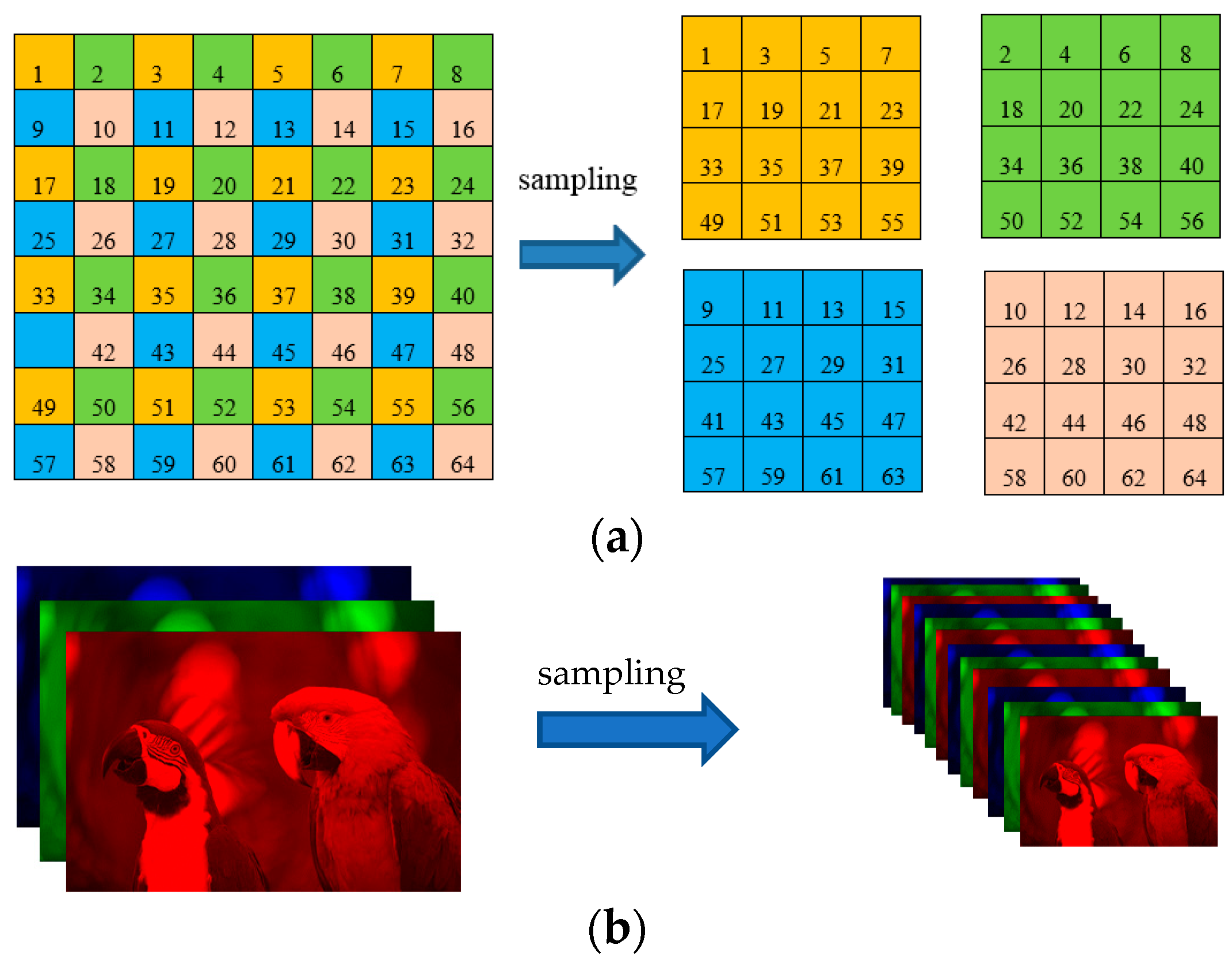
Although the aforesaid representation can approximate a color image, it does not make full use of the similarity of image data. In order to enhance its low-rank property, we sampled an image to obtain four similar images (All sampling factors in this paper are horizontal sampling factor: vertical sampling factor = 2:2), and each image is divided into four sub-images, and there is no pixel overlap between the sub-images, as shown in Figure 2a. Each small square represents a pixel. For a three-channel RGB image, its sampling method is illustrated in Figure 2b.
According to the prior knowledge of image local similarity, the four sub-images are similar, so they are composed of a sub-image tensor which has a low-rank structure. It should be noted that if the pixels of the image rows and columns are not even, we can add one row or one column and then do the down-sampling processing. It can be seen that the tensor representation of the color image kodim23 is A 512 × 768 × 3 in Figure 1. After sampling, we get the sub-image set denoted by A s 256 × 384 × 12 . Here we give the singular values of the tensor bcirc ( A s ) as shown in Figure 1d. Compared with Figure 1c, it can be seen that most of the singular values of the corresponding tensor of the sub-image set appear to be smaller. Therefore, compared with the original whole image, the sub-image data has stronger property of low rank.

3.2. Mode Permutation

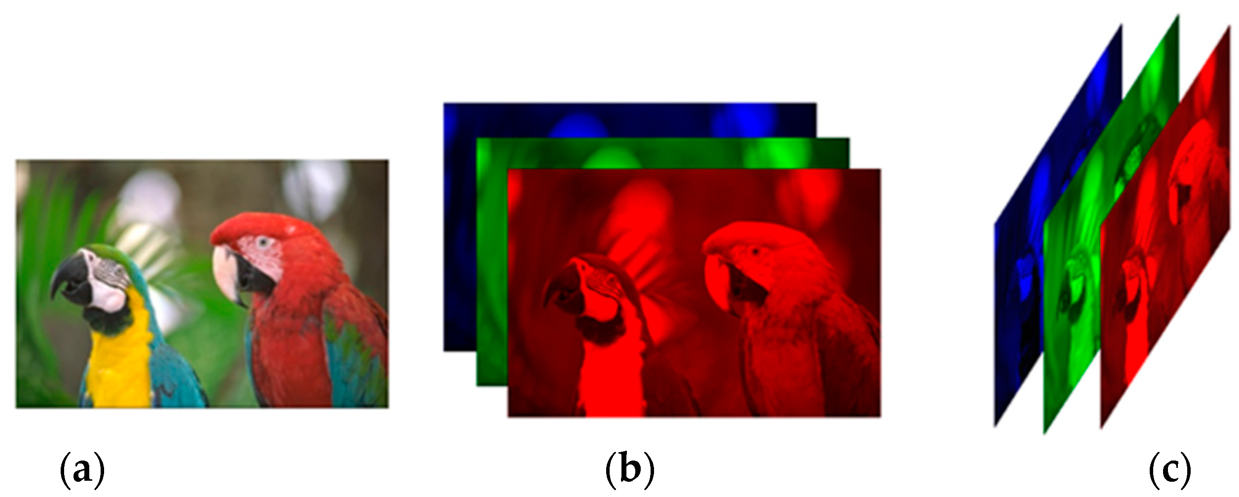
It is important to note that the TNN is orientation-dependent. If the tensor rotates, the value of TNN and the tensor completion results from Formula (1) may be quite different. For example, a three-channel color image of size n 1 × n 2 can be represented as three types of tensors, i.e., X 1 n 1 × n 2 × 3 , X 2 n 1 × 3 × n 2 and X 2 3 × n 1 × n 2 , where X 1 is the most common image tensor representation, X 2 denotes the conjugate transpose of X 2 , and X 1 X 2 , X 2 = X 2 .
In order to further improve the performance, we perform the mode permutation [19] after sampling. Here we give an example of the mode permutation as shown in Figure 3.
In Figure 3, the size of the color image kodim23 is n 1 × n 2 . Its tensor representation is X 1 n 1 × n 2 × 3 . After the mode permutation, it is denoted by X 2 n 1 × 3 × n 2 . So X 2 n 1 × 3 × n 2 is called the mode permutation of X 1 n 1 × n 2 × 3 .
The mode permutation option can avoid scanning an entire image, which reduces the overall computational complexity [19].

3.3. Solution to the Proposed Method

For the completion problem of the color image tensor X N 1 × N 2 × N 3 , we propose a color sub-image tensor X s n 1 × n 2 × n 3 (where n 1 = N 1 / 2 ; n 2 = N 2 / 2 ; n 3 = 4 N 3 ) low-rank optimization model:
arg min X s X s , s . t .   P Ω ( X s ) = P Ω ( M s )
where X s is the tensor nuclear norm of X s , M s and X s are third-order tensors of the same size.
The problem (11) can be solved by the ADMM [20], where the key step is to calculate the proximity operator of the TNN, namely:
p r o x λ   .   ( Y ) = arg min X λ X + 1 2 X Y F 2
According to the literature [18], let Y = U S V be the t-SVD of Y n 1 × n 2 × n 3 , and for each λ > 0 , define the tensor singular value threshold (t-SVT) operator, as follows:
D λ ( Y ) = U S λ V
where S λ = ifft ( ( S ^ λ ) +   , [ ] , 3 ) , ( S ^ λ ) + = max ( ( S ^ λ ) , 0 ) . It is worth noting that the t-SVT operator only needs to apply a soft threshold rule to the singular values S ^ (instead of S ) of the frontal slice of Y ^ . The t-SVT operator is a proximity operator related to TNN.
Based on t-SVT, we exploit the ADMM algorithm to solve the problem of (11). The augmented Lagrangian function of (11) is defined as
L ( L s , Y , μ ) = L s + < Y , L s X s > + μ 2 L s X s F 2
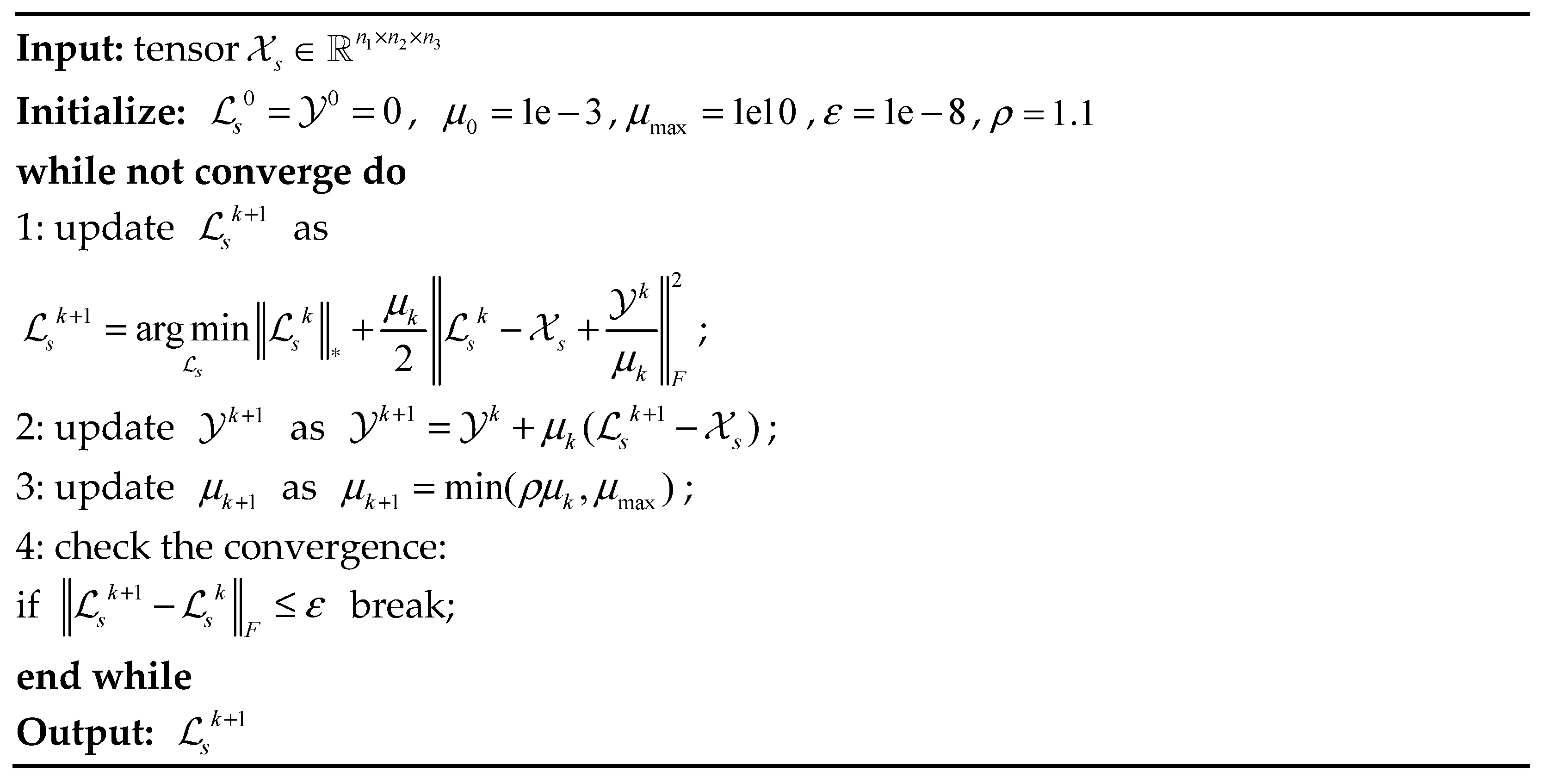
where Y n 1 × n 2 × n 3 is the Lagrangian multiplier and μ > 0 is the penalty parameter. We then update L s by alternately minimizing the augmented Lagrangian function L . The sub-problem has a closed-form solution, with the t-SVT operator related to TNN. A pseudo-code description of the entire optimization problem (11) is given in Figure 4.
In the whole procedure of algorithm SLRTC, the main per-iteration cost lies in the update L s k + 1 , which requires computing fast Fourier transform (FFT) and n 3 + 1 2 SVDS of n 1 × n 2 matrices. The per-iteration complexity is O ( n 1 n 2 n 3 log n 3 + n ( 1 ) n ( 2 ) 2 n 3 ) .
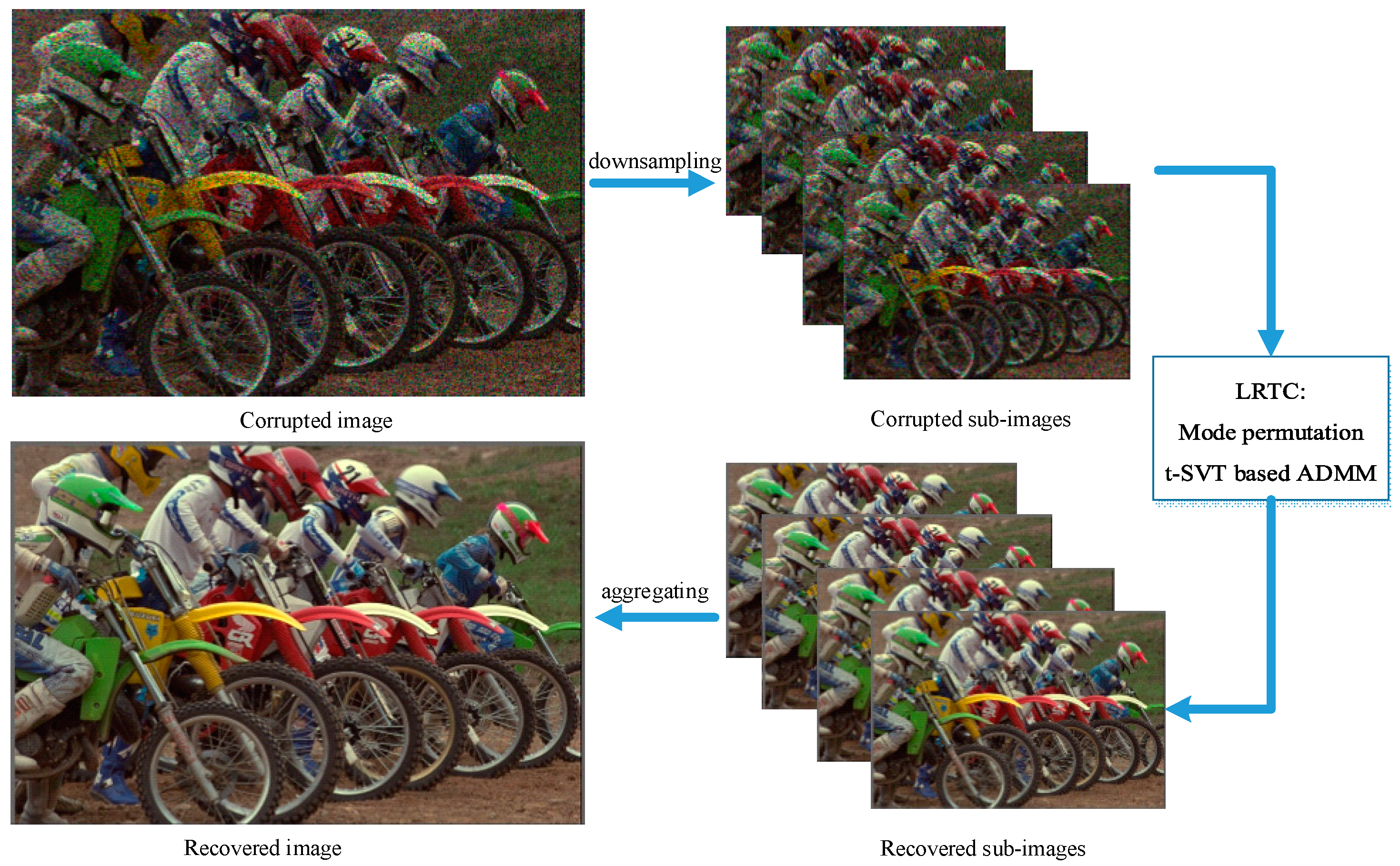
Therefore, the overall framework process of color image restoration based on sub-image low-rank tensor completion proposed is shown in Figure 5.

4. Experiments

In this section, we will compare the proposed SLRTC with several classic color image restoration methods (including FaLRTC [4], LRTC-TNN [5], TCTF [6] and LRTV-TTr1 [7]). Among them, the frontal slice of the input tensor in the LRTC-TNN1 method corresponds to R, G, and B channels, while the lateral slice of the input tensor in the LRTC-TNN2 method corresponds to R, G, and B channels; the LRTC-TNN method is based on TNN, which solves the tensor completion problem by solving the convex optimization.
To evaluate the performance of different methods for color image restoration, we used the widely used peak signal-to-noise ratio (PSNR) and structure similarity (SSIM) [21] indicators in this experiment.

4.1. Color Image Recovery

We first use the original real nine color images for testing, as shown in Figure 6.
The size of each image is 256 × 256 × 3, i.e., row × column × RGB. In order to test the repair effect of various algorithms on the images, we randomly lost 30%, 50%, and 70% of the pixels in each image, and formed an incomplete tensor X 256 × 256 × 3 .
Table 1 lists the PSNR and SSIM comparisons of all methods to restore the images. Compared with the LRTC-TNN1, LRTC-TNN2 and TCTF methods, the SLRTC method can usually obtain the best image restoration results when the missing rate is 30%, 50%, and 70%. By analysing the specific data in Table 1, it can be seen that when the local smoothing in the image accounts for a large proportion, such as Airplane, Pepper and Sailboat, the effect will be better if the LRTV-TTr1 method is utilized to restore the images, because the advantage of TV regularization is to make use of the local smoothness of the image. In addition, when the missing rate is higher (greater than or equal to 70%), the LRTV-TTr1 method is better than SLRTC. When the image contains a large number of texture regions, that is, the image itself has a strong low rank, the best effect can be achieved by applying low rank constraints to the restoration of degraded images, such as facade.
In order to further verify the effectiveness of the proposed algorithm, we additionally used 24 color images from the Kodak PhotoCD dataset (http://r0k.us/graphics/kodak/ (accessed on 3 January 2018)) for testing. The size of each image is 768 × 512 × 3 . As in the previous test, in order to test the repair effect of various algorithms on the image, we randomly lost 30%, 50%, and 70% of the pixels in each image, and formed an incomplete tensor X 768 × 512 × 3 .
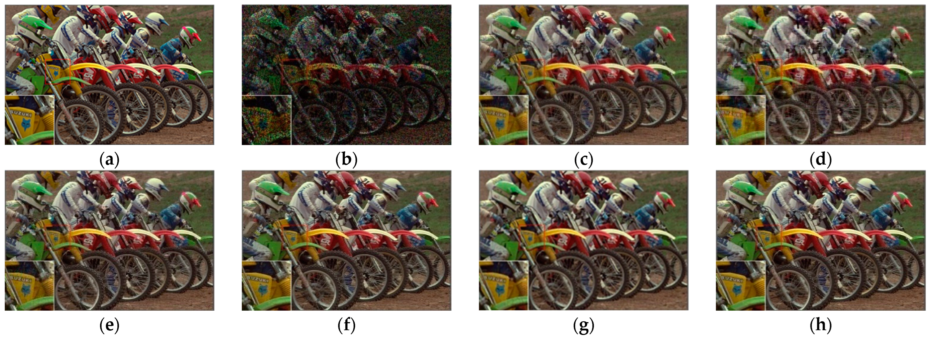
Table 2 lists the PSNR and SSIM comparisons of all methods to restore the images when the missing rate is 30%. The best values among all these methods are in boldface. It can be seen that our algorithm SLRTC can surpass the other algorithms in terms of PSNR, and the PSNR value is about 1.5-5db higher than the other methods. However, in terms of SSIM, it can be seen that the LRTV-TTr1 method is basically optimal.
Table 3 and Table 4 are the comparison of PSNR and SSIM when the missing rate is 50% and 70%, respectively. As shown in Table 2, our algorithm can surpass the other algorithms in terms of PSNR, but the SSIM value of image restoration is lower than that of the LRTC-TTr1 method. The reason is mainly due to the sampling process from image to sub-image in the first step of the SLRTC method. Although the sub-image has a stronger low rank than the original image, it weakens the overall structural relevance of the image.
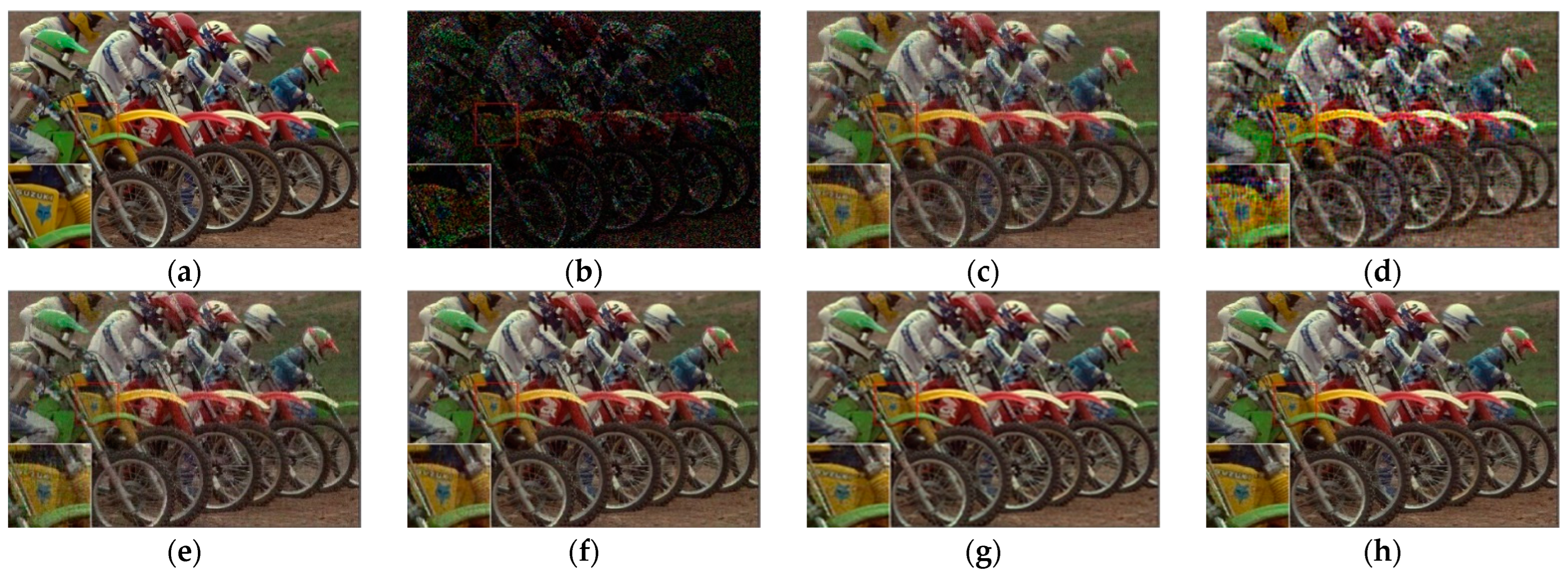
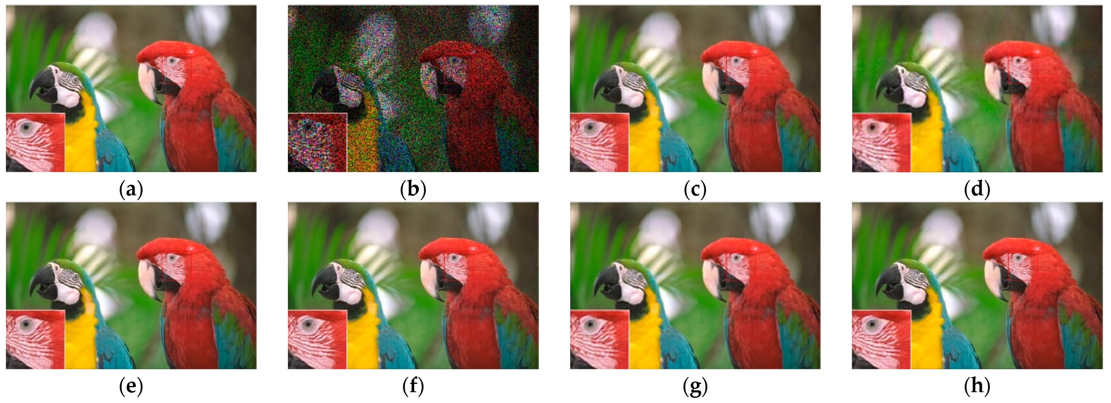
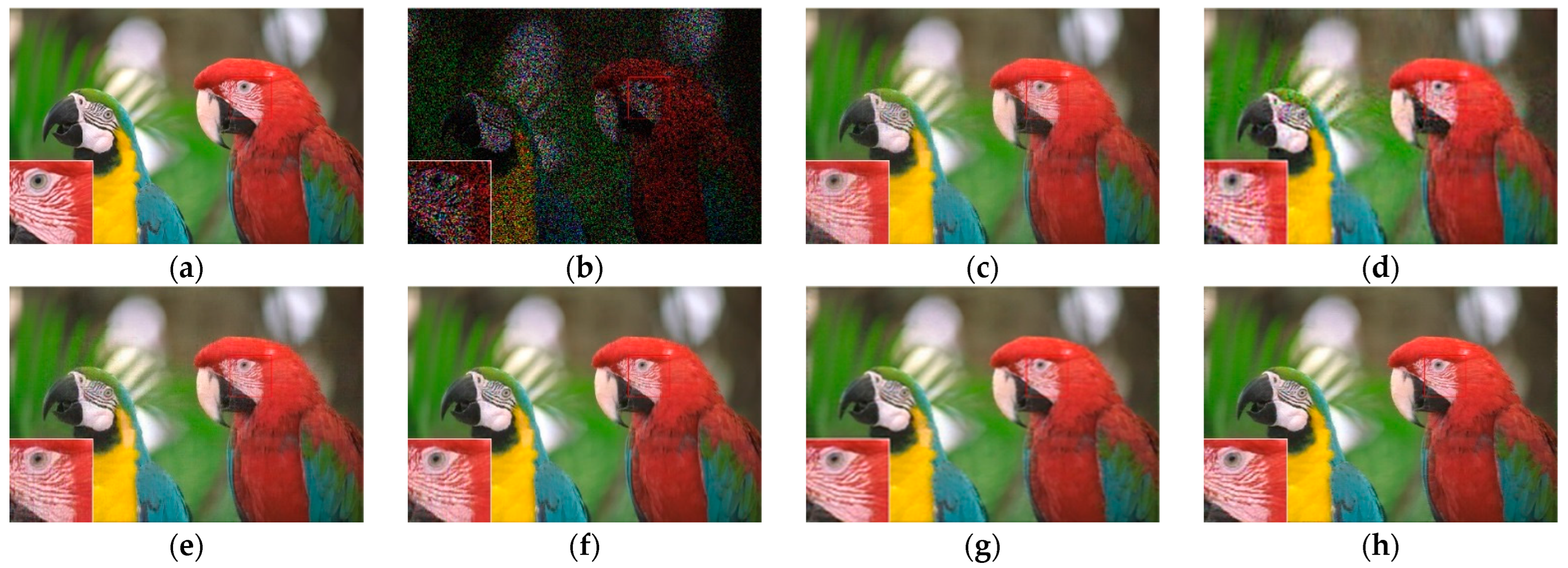
Figure 7, Figure 8, Figure 9 and Figure 10 show the comparison of visual quality when the missing rate is 50% and 70%. In contrast, the SLRTC method can better preserve the texture of the image.
At the same time, we also give a comparison of the algorithm complexity of restoring 24 test images with a resolution of 768 × 512, as shown in Figure 11. It can be seen that SLRTC is much faster than the FaLRTC, LRTC-TNN1, and LRTV-TTr1 methods, and is comparable to the TCTF and LRTC-TNN2 methods.

4.2. Color Video Recovery

Next, we tested the performance of different methods in completing the task of video data. The test video sequences are City, Bus, Crew, Soccer, and Mobile. (https://engineering.purdue.edu/~reibman/ece634/ (accessed on 3 January 2018)).
The main consideration is the third-order tensor. Here, the following preprocessing is performed on each video: adjust the video size of 352 × 288 × 3 × 30 (row × column × RGB × number of frames) to a third-order tensor X 352 × 288 × 90 .
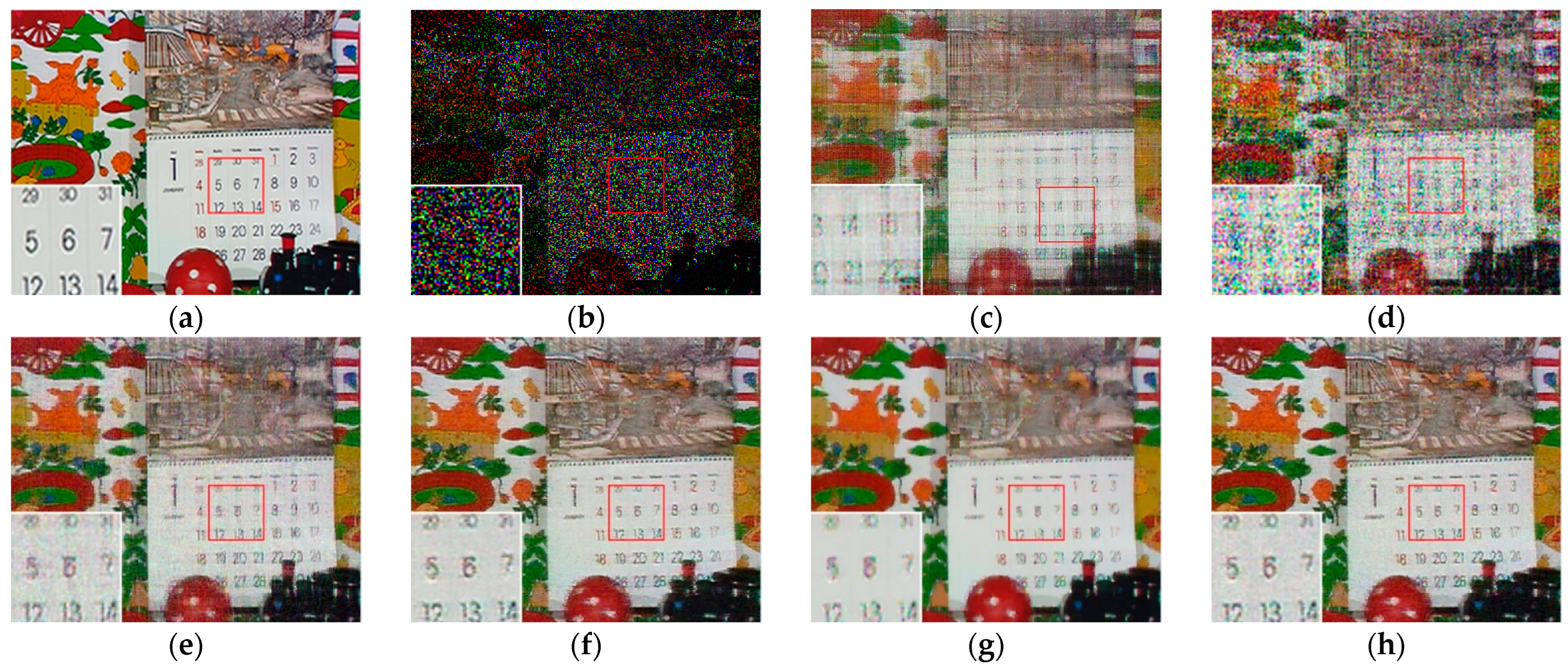
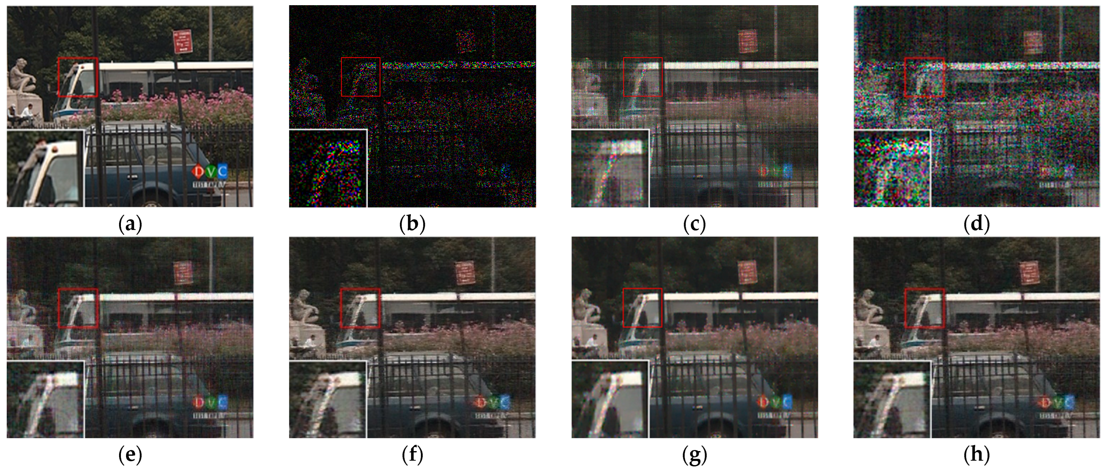
Figure 12, Figure 13, Figure 14 and Figure 15 show the visual quality comparison of the Mobile and Bus video sequences repaired by different methods when the missing rate is 50% and 80%. When the missing rate is 50%, SLRTC can capture the inherent multi-dimensional characteristics of the data, and the video frame recovery effect is better than other methods; when the missing rate is 80%, the subjective visual quality of SLRTC in the Mobile video frame repair is better than other methods, while the subjective visual quality of the repair effect on the Bus video frame is not as good as LRTV_TTr1.
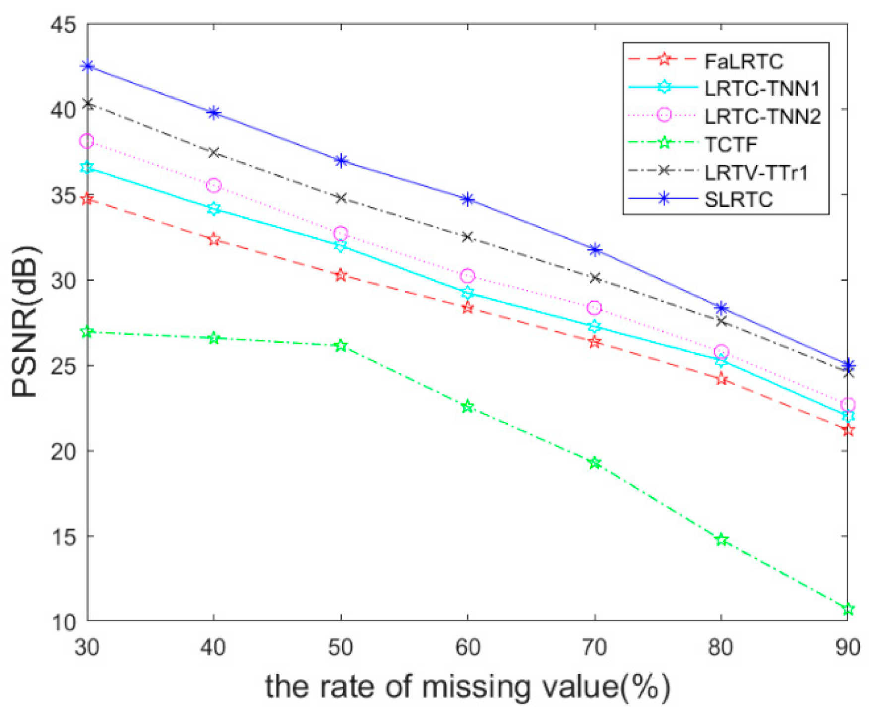
Randomly removing 30%, 40%, 50%, 60%, 70%, 80%, and 90% pixels in the videos, Figure 16 shows the performance comparison of various methods for videos recovery. It can be seen that the SLRTC algorithm proposed is better than other methods.

5. Conclusions

This paper proposes a color image restoration method called SLRTC. Based on the nature of the tensor tubal rank, our method does not minimize the tensor nuclear norm on the observed image, but uses the local similarity characteristics of the image to decompose the image into multiple sub-images through downsampling to enhance the tensor of low rank. Experiments show that the proposed algorithm is better than the comparison algorithms in terms of color image restoration quality and running time.
Obviously, the method proposed in this paper is parameter-independent, and parameter adjustment usually requires complex calculations. In the absence of TV regularization terms, the method proposed in this paper uses the image partial smoothing prior to downsampling the image. It is well integrated into the sub-image low-rank tensor completion, and the effectiveness of the model is proved through experiments.
Since deep learning-based algorithms have shown their potential to tackle this problem of image restoration in recent years [22,23], we next will integrate the low-rank prior into the neural networks to achieve better performance.

Author Contributions

Conceptualization, X.L. and G.T.; Methodology, X.L.; Software, X.L.; Writing—original draft, X.L.; Writing—review and editing X.L. and G.T. All authors have read and agreed to the published version of the manuscript.

Funding

This work was supported by the Postgraduate Research & Practice Innovation Program of Jiangsu Province (KYCX17_0776), and the Research Project of Nanjing University of Posts and Telecommunications (NY218089).

Institutional Review Board Statement

Not applicable.

Informed Consent Statement

Not applicable.

Data Availability Statement

Data available on request from the authors.

Conflicts of Interest

The authors declare no conflict of interest.

References

  1. Zhang, C.; Hu, W.; Jin, T.; Mei, Z. Nonlocal image denoising via adaptive tensor nuclear norm minimization. Neural Comput. Appl. 2015, 29, 3–19. [Google Scholar] [CrossRef]
  2. Rajwade, A.; Rangarajan, A.; Banerjee, A. Image Denoising Using the Higher Order Singular Value Decomposition. IEEE Trans. Pattern Anal. Mach. Intell. 2009, 35, 849–862. [Google Scholar] [CrossRef] [PubMed]
  3. Kolda, T.G.; Bader, B.W. Tensor Decompositions and Applications. SIAM Rev. 2009, 51, 455–500. [Google Scholar] [CrossRef]
  4. Liu, J.; Musialski, P.; Wonka, P.; Ye, J. Tensor Completion for Estimating Missing Values in Visual Data. IEEE Trans. Pattern Anal. Mach. Intell. 2013, 35, 208–220. [Google Scholar] [CrossRef] [PubMed]
  5. Lu, C.; Feng, J.; Lin, Z.; Yan, S. Exact Low Tubal Rank Tensor Recovery from Gaussian Measurements. In Proceedings of the International Joint Conference on Artificial Intelligence, Stockholm, Sweden, 13–19 July 2018; pp. 1948–1954. [Google Scholar]
  6. Zhou, P.; Lu, C.; Lin, Z.; Zhang, C. Tensor Factorization for Low-Rank Tensor Completion. IEEE Trans. Image Process. 2018, 27, 1152–1163. [Google Scholar] [CrossRef] [PubMed]
  7. Liu, X.; Jing, X.Y.; Tang, G.; Wu, F.; Dong, X. Low-rank tensor completion for visual data recovery via the tensor train rank-1 decomposition. IET Image Process. 2020, 14, 114–124. [Google Scholar] [CrossRef]
  8. Kilmer, M.E.; Martin, C.D. Factorization Strategies for Third-order Tensors. Linear Algebra Appl. 2011, 435, 641–658. [Google Scholar] [CrossRef]
  9. Kilmer, M.E.; Braman, K.; Hao, N.; Hoover, R.C. Third-order Tensors as Operators on Matrices: A Theoretical and Computational Framework with in Imaging. SIAM J. Matrix Anal. Appl. 2013, 34, 148–172. [Google Scholar] [CrossRef]
  10. Martin, C.D.; Shafer, R.; LaRue, B. An order-p Tensor Factorization with Applications in Imaging. SIAM J. Sci. Comput. 2013, 35, A474–A490. [Google Scholar] [CrossRef]
  11. Lu, C.; Feng, J.; Chen, Y.; Liu, W.; Lin, Z.; Yan, S. Tensor robust Principal Component Analysis: Exact Recovery of Corrupted Low-rank Tensors via Convex Optimization. In Proceedings of the Conference on Computer Vision and Pattern Recognition, Las Vegas, NV, USA, 27–30 June 2016; pp. 5249–5257. [Google Scholar]
  12. Semerci, O.; Hao, N.; Kilmer, M.E.; Miller, E.L. Tensor-based Formulation and Nuclear Norm Regularization for Multienergy Computed Tomography. IEEE Trans. Image Process. 2014, 23, 1678–1693. [Google Scholar] [CrossRef] [PubMed] [Green Version]
  13. Sun, W.; Huang, L.; So, H.C.; Wang, J. Orthogonal Tubal Rank-1 Tensor Pursuit for Tensor Completion. Signal Process. 2019, 157, 213–224. [Google Scholar] [CrossRef]
  14. Sun, W.; Chen, Y.; Huang, L.; So, H.C. Tensor Completion via Generalized Tensor Tubal Rank Minimization using General Unfolding. IEEE Signal Process. Lett. 2018, 25, 868–872. [Google Scholar] [CrossRef]
  15. Long, Z.; Liu, Y.; Chen, L.; Zhu, C. Low Rank Tensor Completion for Multiway Visual Data. Signal Process. 2019, 155, 301–316. [Google Scholar] [CrossRef]
  16. Zhang, Z.; Ely, G.; Aeron, S.; Hao, N.; Kilmer, M. Novel methods for multilinear data completion and denoising based on tensor-SVD. In Proceedings of the IEEE Conference on Computer Vision and Pattern Recognition, Columbus, OH, USA, 23–28 June 2014; pp. 3842–3849. [Google Scholar]
  17. Wang, A.; Song, X.; Wu, X.; Lai, Z.; Jin, Z. Generalized Dantzig Selector for Low-tubal-rank Tensor Recovery. In Proceedings of the IEEE International Conference on Acoustics, Speech and Signal Processing, Brighton, UK, 12–17 May 2019; pp. 3427–3431. [Google Scholar]
  18. Lu, C.; Feng, J.; Chen, Y.; Liu, W.; Lin, Z.; Yan, S. Tensor Robust Principal Component Analysis with A New Tensor Nuclear Norm. IEEE Trans. Pattern Anal. Mach. Intell. 2020, 42, 925–938. [Google Scholar] [CrossRef] [PubMed]
  19. Zdunek, R.; Fonal, K.; Sadowski, T. Image Completion with Filtered Low-Rank Tensor Train Approximations. In Proceedings of the International Work-Conference on Artificial Neural Networks, Part II, Gran Canaria, Spain, 12–14 June 2019; pp. 235–245. [Google Scholar]
  20. Lu, C.; Feng, J.; Yan, S.; Lin, Z. A Unified Alternating Direction Method of Multipliers by Majorization Minimization. IEEE Trans. Pattern Anal. Mach. Intell. 2018, 40, 527–541. [Google Scholar] [CrossRef] [PubMed]
  21. Wang, Z.; Bovik, A.C.; Sheikh, H.R.; Simoncelli, E.P. Image quality assessment: From error visibility to structural similarity. IEEE Trans. Image Process. 2004, 13, 600–612. [Google Scholar] [CrossRef] [PubMed]
  22. Zhang, K.; Ren, W.; Luo, W.; Lai, W.S.; Stenger, B.; Yang, M.H.; Li, H. Deep image deblurring: A survey. Int. J. Comput. Vis. 2022, 130, 2103–2130. [Google Scholar] [CrossRef]
  23. Zamir, S.W.; Arora, A.; Khan, S.; Hayat, M.; Khan, F.S.; Yang, M.H.; Shao, L. Multi-stage progressive image restoration. In Proceedings of the IEEE Conference on Computer Vision and Pattern Recognition, Nashville, TN, USA, 20–25 June 2021; pp. 14821–14831. [Google Scholar]
Figure 1. Color image and its singular values. (a) Color Image kodim23 denoted by X 512 × 768 × 3 ; (b) Color sub-image set denoted by X s 256 × 384 × 12 ; (c) the singular values of bcirc ( X ) ; (d) the singular values of bcirc ( X s ) .
Sensors 23 01706 g001
Figure 2. A simple demonstration of the sampling method. (a) An image is sampled to obtain four sub-images; (b) A three-channel RGB image is sampled to form four three-channel sub-images.
Sensors 23 01706 g002
Figure 3. Two tensor representations of a color image. (a) image kodim23; (b) X 1 n 1 × n 2 × 3 ; (c) X 2 n 1 × 3 × n 2 .
Sensors 23 01706 g003
Figure 4. Our algorithm SLRTC.
Sensors 23 01706 g004
Figure 5. Flowchart of the proposed framework. The downsampling method is as shown in Section 3.1. After the mode permutation of the sub-images, t-SVT is performed to obtain the recovered sub-images. Finally, the final recovered image can be obtained by aggregating the recovered sub-images.
Sensors 23 01706 g005
Figure 6. Ground truth of nine benchmark color images: Airplane, Baboon, Barbara, Façade, House, Peppers, Sailboat, Giant and Tiger (from left to right).
Sensors 23 01706 g006
Figure 7. Visual effect comparison of different methods on the color image kodim05. The incomplete image contains 50% missing entries, shown as black pixels. (a) Original image; (b) Incomplete image; (c) FaLRTC (26.01 dB); (d) TCTF (22.45 dB); (e)LRTC-TNN1 (28.34 dB); (f) LRTC-TNN2 (29.98 dB); (g) LRTV-TTr1 (29.08 dB); (h) SLRTC (31.93 dB).
Sensors 23 01706 g007
Figure 8. Visual effect comparison of different methods on the color image kodim05. The incomplete image contains 70% missing entries, shown as black pixels. (a) Original image; (b) Incomplete image; (c) FaLRTC (21.80 dB); (d) TCTF (19.41 dB); (e) LRTC-TNN1 (22.67 dB); (f) LRTC-TNN2 (24.59 dB); (g) LRTV-TTr1 (24.48 dB); (h) SLRTC (26.14 dB).
Sensors 23 01706 g008
Figure 9. Visual effect comparison of different methods on the color image kodim23. The incomplete image contains 50% missing entries, shown as black pixels. (a) Original image; (b) Incomplete image; (c) FaLRTC (33.35 dB); (d) TCTF (29.21 dB); (e) LRTC-TNN1 (33.47dB); (f) LRTC-TNN2 (33.72 dB); (g) LRTV-TTr1 (34.46dB); (h) SLRTC (37.96dB).
Sensors 23 01706 g009
Figure 10. Visual effect comparison of different methods on the color image kodim23. The incomplete image contains 70% missing entries, shown as black pixels. (a) Original image; (b) Incomplete image; (c) FaLRTC (29.09 dB); (d) TCTF (26.94 dB); (e) LRTC-TNN1 (28.94 dB); (f) LRTC-TNN2 (29.14 dB); (g) LRTV-TTr1 (30.89 dB); (h) SLRTC (32.33 dB).
Sensors 23 01706 g010
Figure 11. Comparison of the running time.
Sensors 23 01706 g011
Figure 12. Visual effect comparison of different methods on the ninth frame completion of the Mobile video. The incomplete video contains 50% missing entries. (a) Original image; (b) Incomplete image; (c) FaLRTC (21.51 dB); (d) TCTF (21.80 dB); (e) LRTC-TNN1 (24.12 dB); (f) LRTC-TNN2 (28.09dB); (g) LRTV-TTr1 (26.15 dB); (h) SLRTC (29.97 dB).
Sensors 23 01706 g012
Figure 13. Visual effect comparison of different methods on the ninth frame completion of the Mobile video. The incomplete video contains 80% missing entries. (a) Original image; (b) Incomplete image; (c) FaLRTC (16.46 dB); (d) TCTF (11.53 dB); (e) LRTC-TNN1 (18.69 dB); (f) LRTC-TNN2 (20.67dB); (g) LRTV-TTr1 (19.91 dB); (h) SLRTC (20.87 dB).
Sensors 23 01706 g013
Figure 14. Visual effect comparison of different methods on the ninth frame completion of the Bus video. The incomplete video contains 50% missing entries. (a) Original image; (b) Incomplete image; (c) FaLRTC (27.30 dB); (d) TCTF (26.42 dB); (e) LRTC-TNN1 (29.05 dB); (f) LRTC-TNN2 (32.92 dB); (g) LRTV-TTr1 (31.77 dB); (h) SLRTC (34.34 dB).
Sensors 23 01706 g014aSensors 23 01706 g014b
Figure 15. Visual effect comparison of different methods on the ninth frame completion of the Bus video. The incomplete video contains 80% missing entries. (a) Original image; (b) Incomplete image; (c) FaLRTC (21.42 dB); (d) TCTF (14.00 dB); (e) LRTC-TNN1 (22.51 dB); (f) LRTC-TNN2 (24.86 dB); (g) LRTV-TTr1 (23.99 dB); (h) SLRTC (24.69 dB).
Sensors 23 01706 g015
Figure 16. The PSNR metric on video data recovery.
Sensors 23 01706 g016
Table 1. The PSNR and SSIM Comparison of different methods on nine images (The best results are highlighted).
Test
Images
MissngrateFaLRTC [4]LRTC-TNN1 [5]LRTC-TNN2 [5]TCTF [6] LRTV-TTr1 [7]SLRTC
PSNRSSIMPSNRSSIMPSNRSSIMPSNRSSIMPSNRSSIMPSNRSSIM
Airplane30%34.720.97334.340.96734.340.97429.480.91937.730.99136.350.981
50%29.790.91929.230.90630.230.94026.770.84932.900.97131.530.951
70%25.240.79424.680.77726.120.85818.630.52228.570.92427.070.875
Baboon30%28.190.92828.620.92930.150.95426.300.89229.800.95530.760.961
50%24.750.82024.840.82126.230.87523.810.77326.230.87326.890.889
70%22.000.64421.600.62922.710.71417.000.39423.600.73123.310.730
Barbara30%34.570.97337.550.98336.410.98229.720.92437.520.98038.690.989
50%29.760.91930.860.92630.430.93027.490.85832.450.95632.500.954
70%25.390.79525.400.78425.610.80619.790.57228.380.88927.360.856
Facade30%37.580.98939.200.99236.820.98935.220.98037.710.98938.710.992
50%33.490.96934.600.97331.590.96030.360.94633.210.96633.350.971
70%29.770.92530.420.93127.320.89020.840.71829.070.90128.540.909
House30%30.080.97730.810.95930.020.96232.260.94130.260.98238.450.984
50%28.680.93829.140.91328.730.93030.060.88629.370.95734.200.958
70%26.170.84426.140.80026.550.85919.650.51727.940.91229.880.893
Peppers30%31.340.94930.860.93130.120.93826.740.84934.640.98134.300.970
50%27.660.88226.530.83926.590.87225.740.81030.790.95629.960.930
70%23.640.73322.060.65622.790.73318.990.51527.170.90525.760.831
Sailboat30%31.540.95931.050.94832.330.96927.530.89833.690.98133.470.976
50%27.160.88926.740.86927.870.91524.880.80829.680.95029.070.933
70%23.130.74222.750.71123.940.79517.560.48726.020.88225.100.830
Giant30%30.010.95331.370.96032.130.97427.070.90532.220.97833.040.979
50%25.720.87426.650.87727.510.91924.400.81328.050.93728.340.932
70%22.030.71722.460.71323.440.79717.650.50224.500.84424.250.818
Tiger30%33.160.97637.580.98837.550.99128.390.91836.970.99039.290.994
50%27.890.91430.120.93630.650.95525.190.82331.130.95832.390.969
70%23.340.76324.330.77925.130.84318.010.51626.550.87326.480.877
Table 2. The PSNR and SSIM Comparison of different methods on the Kodak PhotoCD dataset, the incomplete images tested contain 30 percent missing entries (The best results are highlighted).
Test
Images
FaLRTC [4]LRTC-TNN1 [5]LRTC-TNN2 [5]TCTF [6]LRTV-TTr1 [7]SLRTC
PSNRSSIMPSNRSSIMPSNRSSIMPSNRSSIMPSNRSSIMPSNRSSIM
kodim0133.570.98939.680.99039.060.99129.030.92735.980.99741.010.994
kodim0238.420.99241.800.98741.310.98933.280.94238.580.99644.390.994
kodim0338.330.99440.750.98742.680.99531.870.92437.820.99744.640.996
kodim0438.160.99340.920.98634.280.98431.760.92137.890.99743.580.994
kodim0531.120.98935.820.98336.670.99024.800.85833.990.99638.980.994
kodim0634.570.98939.600.98941.200.99529.760.92536.020.99642.200.996
kodim0737.710.99641.080.99042.340.99530.130.91037.640.99844.410.996
kodim0831.630.99137.020.98734.590.98725.450.89734.950.99737.820.993
kodim0938.490.99542.380.99034.330.98732.380.94338.110.99843.850.995
kodim1037.450.99441.530.98934.000.98731.900.93537.950.99843.430.995
kodim1134.830.99139.480.98840.390.99330.370.92936.400.99642.180.995
kodim1239.110.99443.000.99042.590.99434.100.94638.710.99744.800.995
kodim1329.230.98134.580.98236.300.98925.090.88532.610.99337.070.991
kodim1433.180.98936.350.98137.920.99027.510.89034.700.99539.830.993
kodim1537.090.99240.390.98538.970.98731.000.92338.010.99742.030.993
kodim1638.770.99343.400.99245.510.99633.280.94437.720.99746.230.997
kodim1736.720.99440.560.98941.690.99431.140.92541.310.99842.790.995
kodim1832.570.98736.620.98036.910.98727.890.88836.500.99638.600.991
kodim1936.340.99240.810.98839.060.99030.860.92740.600.99741.810.994
kodim2036.560.99440.020.98840.730.99231.080.93937.770.99842.120.994
kodim2134.770.99339.060.98740.730.99329.060.92435.980.99741.580.994
kodim2235.790.99038.930.98338.300.98630.780.91536.880.99540.160.990
kodim2337.390.99636.610.99037.590.98931.660.92137.130.99844.170.994
kodim2431.510.98734.760.97835.680.98627.170.89635.280.99636.770.990
Table 3. The PSNR and SSIM Comparison of different methods on the Kodak PhotoCD dataset, the incomplete images tested contain 50 percent missing entries (The best results are highlighted).
Test
Images
FaLRTC [4]LRTC-TNN1 [5]LRTC-TNN2 [5]TCTF [6]LRTV-TTr1 [7]SLRTC
PSNRSSIMPSNRSSIMPSNRSSIMPSNRSSIMPSNRSSIMPSNRSSIM
kodim0129.050.95932.580.94832.310.95826.670.85131.820.98434.010.970
kodim0233.840.97135.220.94435.430.96031.590.89035.360.98537.670.972
kodim0333.770.97534.640.94437.050.97729.500.86935.100.98939.050.983
kodim0433.300.97134.340.93932.330.95729.360.85735.310.98837.050.972
kodim0526.010.94928.340.90529.980.95022.450.74229.080.98131.930.967
kodim0629.810.95832.800.94634.920.97627.200.84931.920.98135.670.979
kodim0732.520.98134.000.95235.590.97527.780.84734.190.99237.650.984
kodim0826.740.96329.740.93328.070.93923.060.80630.000.98630.840.965
kodim0933.550.98135.660.95832.210.96629.950.89235.330.99237.110.978
kodim1032.660.97634.800.95031.900.96329.480.87734.700.99236.890.978
kodim1130.310.96532.650.94033.940.96727.900.85832.560.98435.380.974
kodim1234.210.97536.190.95636.600.97531.620.89635.230.98738.670.981
kodim1324.860.92727.910.90830.020.94922.470.76327.710.96830.620.957
kodim1428.530.95629.600.91031.710.95625.110.79330.470.97933.350.967
kodim1532.430.97233.830.93633.080.95328.650.86434.650.98935.960.970
kodim1633.970.97336.840.96439.390.98330.890.88734.890.98839.950.985
kodim1732.230.97534.580.95336.060.97528.690.85836.430.99337.340.981
kodim1828.040.95129.990.90830.890.94425.500.78831.290.98132.470.961
kodim1931.680.97134.170.94932.500.96028.500.86135.210.98835.110.972
kodim2031.510.97533.640.95034.720.97128.640.88433.950.99136.130.977
kodim2129.710.97132.410.94334.520.97226.700.85631.950.98735.340.976
kodim2231.310.96332.870.93132.910.94828.380.83933.100.98134.560.963
kodim2333.350.98533.470.96033.720.96429.210.87334.460.99237.960.978
kodim2427.100.95129.100.90830.470.94524.750.79930.310.98431.450.959
Table 4. The PSNR and SSIM Comparison of different methods on the Kodak PhotoCD dataset, the incomplete images tested contain 70 percent missing entries (The best results are high-lighted).
Test
Images
FaLRTC [4]LRTC-TNN1 [5]LRTC-TNN2 [5]TCTF [6]LRTV-TTr1 [7]SLRTC
PSNRSSIMPSNRSSIMPSNRSSIMPSNRSSIMPSNRSSIMPSNRSSIM
kodim0125.420.87626.840.81926.980.85722.920.69927.200.93228.290.886
kodim0230.240.91930.460.84831.000.89428.800.79631.670.95032.600.913
kodim0329.690.92429.480.84131.630.92227.480.77231.110.96333.590.942
kodim0429.050.91029.120.82229.370.88426.110.73831.180.95631.660.911
kodim0521.800.82722.670.71124.590.83219.410.53824.480.92526.140.874
kodim0626.090.87127.480.82829.780.92123.190.69427.740.92730.240.924
kodim0727.850.92728.350.84929.930.91324.710.72630.070.97131.860.939
kodim0822.470.88123.880.79122.930.81520.180.66425.120.94624.890.867
kodim0928.990.93629.960.87428.710.90525.610.78631.080.97131.340.927
kodim1028.650.92329.420.85028.820.90225.590.75930.940.97131.520.928
kodim1126.560.89727.380.82228.710.89323.700.71428.430.94229.740.906
kodim1230.140.92630.890.87231.340.92527.370.78531.660.95733.030.935
kodim1321.490.79122.780.72225.040.83718.820.55023.540.88625.450.852
kodim1424.570.85624.590.74026.690.85922.420.62326.340.92428.020.883
kodim1528.280.91728.580.82328.150.86526.140.76130.470.96330.580.905
kodim1630.000.91331.250.87534.030.94226.380.74331.090.95034.350.945
kodim1728.110.91429.240.85330.850.91524.330.71831.670.97232.170.936
kodim1824.420.85025.060.74326.260.83421.350.59827.020.93227.630.873
kodim1927.500.91028.610.84127.260.87724.810.73630.320.95829.180.904
kodim2027.400.92528.340.85729.920.91924.760.77729.850.97031.260.932
kodim2125.640.90526.890.83129.230.91422.640.71527.680.95229.830.920
kodim2227.550.88727.990.80328.360.85325.090.69429.230.93529.720.883
kodim2329.090.95128.940.88029.140.89826.940.81730.890.97632.330.932
kodim2423.610.85724.470.75226.000.84021.210.60726.230.94126.840.869
Disclaimer/Publisher’s Note: The statements, opinions and data contained in all publications are solely those of the individual author(s) and contributor(s) and not of MDPI and/or the editor(s). MDPI and/or the editor(s) disclaim responsibility for any injury to people or property resulting from any ideas, methods, instructions or products referred to in the content.