
Small Sample Coherent DOA Estimation Method Based on S2S Neural Network Meta Reinforcement Learning

Abstract
1. Introduction
2. MDP Model for Coherent DOA Estimation
2.1. Quadratic Feature Extraction of Coherent DOA Estimation
2.2. MDP Model for Coherent DOA Estimation
2.2.1. Definition of the State Space S
2.2.2. Definition of Action Space A
2.2.3. Definition of State Transfer Gain
3. DOA Estimation Based on S2S Network Meta−Reinforcement Learning Algorithm
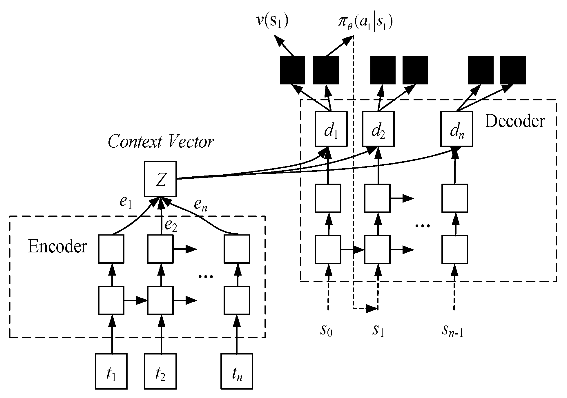
3.1. Expression of S2S Deep Neural Network
3.2. The Optimal Strategy Algorithm Based on Meta−Reinforcement Learning
| Algorithm 1 The Optimal Strategy Training Algorithm Based on Meta−reinforcement Learning |
| 1: . 2: . do. . , do. 6: of the network parameters. being the inner MDP learning rate. 8: After each task of the sequence converges, the system state is updated and the strategy learning for the next task proceeds. The parameters of the convergence strategy corresponding to each task of this sequence are saved. 9: End for. 10: The saved network parameters learned from the previous sequence are passed to the outer loop to train the hyper-parameters. 11: is the outer learning rate, which is a balanced parameter for exploration and exploitation. 12: End for. |
4. Experiments and Analysis of Results
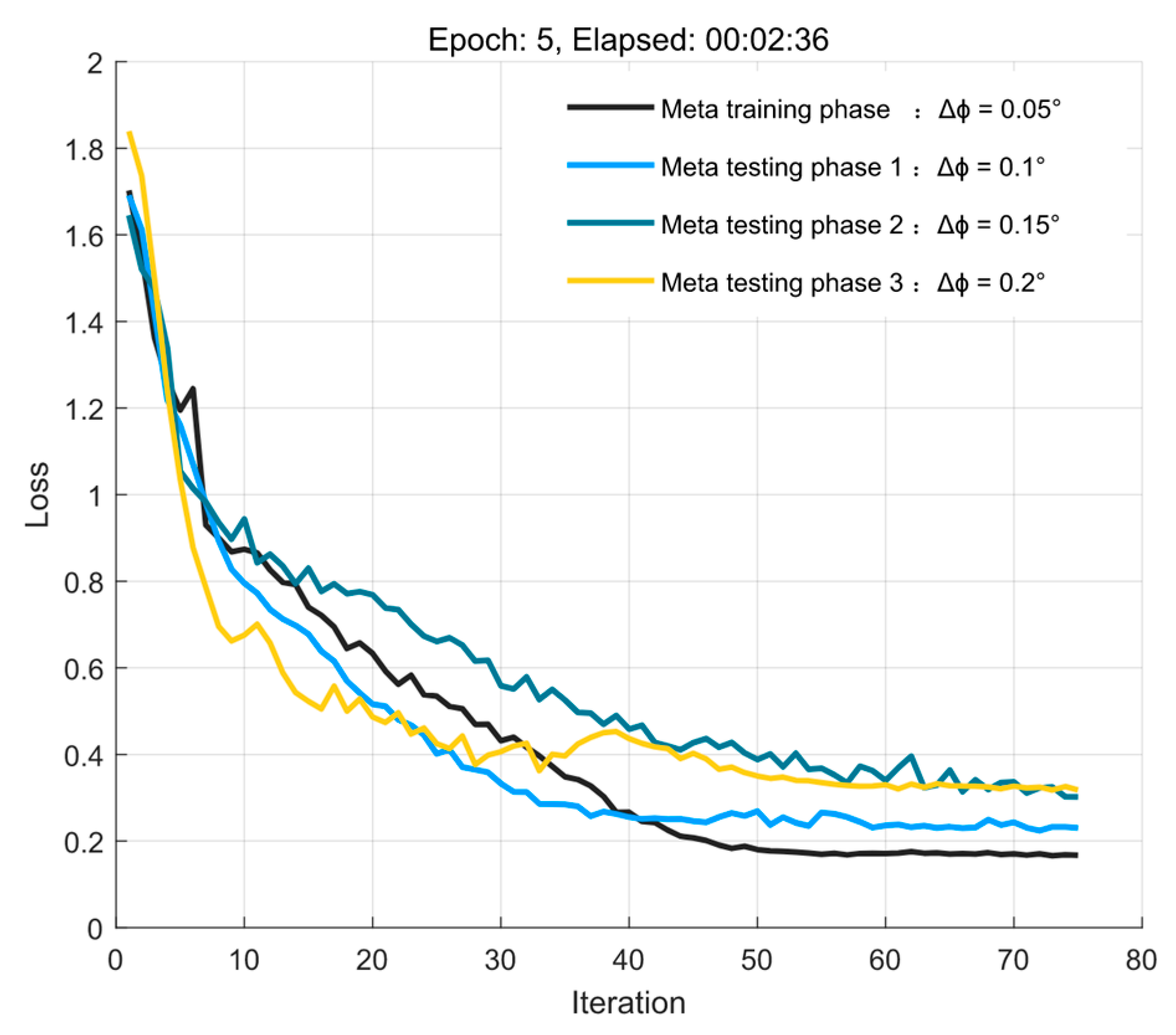
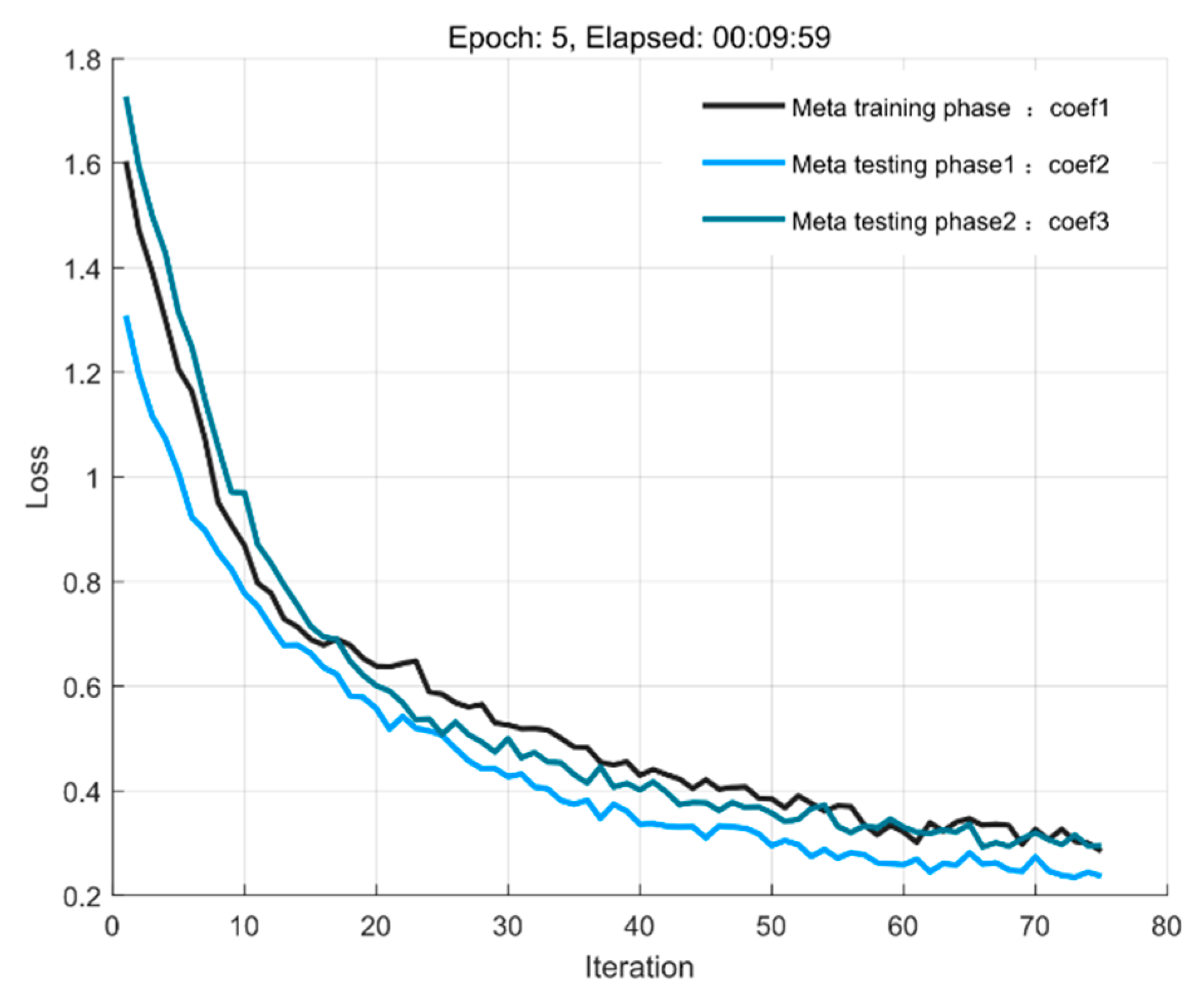
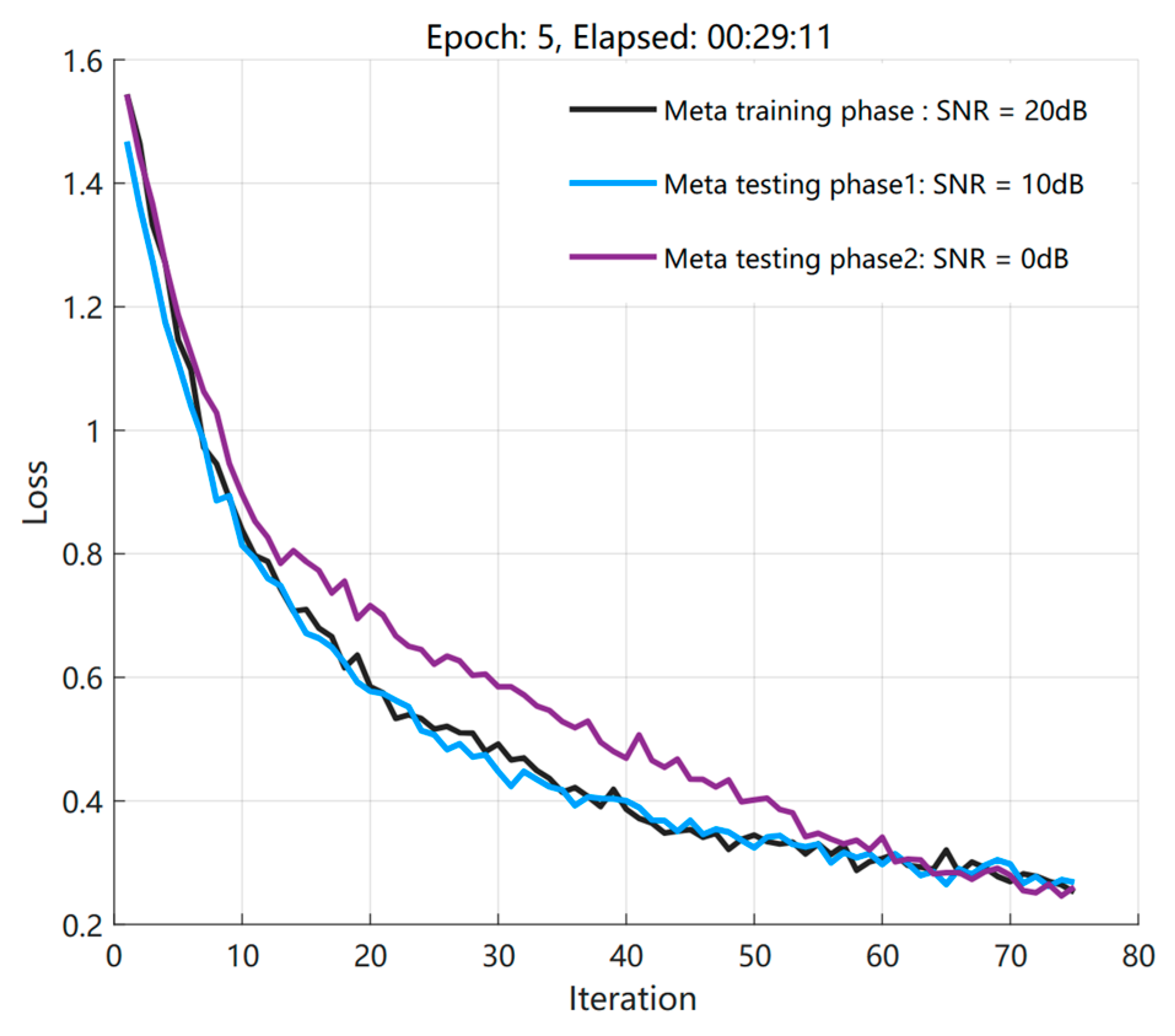
4.1. Loss Function Trained under Different Influences
4.2. Performance Testing in the Original Environment Based on the Meta−Training Phase
4.3. Performance Testing in New Environments Based on Meta−Testing Phases
4.4. Comparison of Test Sample Cost
4.5. Calculation Complexity and Test Time Analysis
- Calculation complexity
- B.
- Test-time analysis
5. Conclusions
Author Contributions
Funding
Institutional Review Board Statement
Informed Consent Statement
Data Availability Statement
Acknowledgments
Conflicts of Interest
References
- Schmidt, R.O. Multiple emitter location and signal parameter estimation. IEEE Trans. Antennas Propag. 1986, 34, 276–280. [Google Scholar] [CrossRef]
- Haykin, S.; Greenlay, T.; Litva, J. Performance evaluation of the modified FBLP method for angle of arrival estimation using real radar multipath data. IEE Proc. F Commun. Radar Signal Process. 1985, 132, 159–174. [Google Scholar] [CrossRef]
- Shan, T.-J.; Wax, M.; Kailath, T. On spatial smoothing for direction-of-arrival estimation of coherent signals. IEEE Trans. Acoust. Speech Signal Process. 1985, 33, 806–811. [Google Scholar] [CrossRef]
- Rao, B.D.; Hari KV, S. Weighted subspace methods and spatial smoothing: Analysis and comparison. IEEE Trans. Signal Process. 1993, 41, 788–803. [Google Scholar] [CrossRef]
- Roy, R.; Kailath, T. ESPRIT-estimation of signal parameters via rotational invariance techniques. IEEE Trans. Acoust. Speech Signal Process. 1989, 37, 984–995. [Google Scholar] [CrossRef]
- Shan, T.J.; Wax, M. Adaptive beamforming for coherent signals and interference. IEEE Trans. Acoust. Speech Signal Process. 1985, 33, 527–536. [Google Scholar] [CrossRef]
- Choi, Y.H. On conditions for the rank restoration in forward backward spatial smoothing. IEEE Trans. Signal Process. 2002, 50, 2900–2901. [Google Scholar] [CrossRef]
- Choi, Y.H. Subspace-based coherent source localization with forward/backward covariance matrices. IEE Proc. Radar Sonar Navig. 2002, 149, 145–151. [Google Scholar] [CrossRef]
- Du, W.X.; Kirlin, R.L. Improved Spatial Smoothing Techniques for DOA Estimation of Coherent Signals. IEEE Trans Signal Process. 1991, 39, 1208–1210. [Google Scholar] [CrossRef]
- Rohwer, J.A.; Abdallah, C.T. One-vs-One Multiclass Least Squares Support Vector Machines for Direction of Arrival Estimation. Appl. Comput. Electromagn. Soc. J. 2003, 18, 345–354. [Google Scholar]
- Christodoulou, C.G.; Rohwer, J.A.; Abdallah, C.T. The use of machine learning in smart antennas. IEEE Antennas Propag. Soc. Symp. 2004, 1, 321–324. [Google Scholar] [CrossRef]
- Donelli, M.; Viani, F.; Rocca, P.; Massa, A. An Innovative Multiresolution Approach for DOA Estimation Based on a Support Vector Classification. IEEE Trans. Antennas Propag. 2009, 57, 2279–2292. [Google Scholar] [CrossRef]
- Du, J.X.; Feng, X.A.; Ma, Y. DOA estimation based on support vector machine-Large scale multiclass classification problem. IEEE Int. Conf. Signal Process. Commun. Comput. 2011, 57, 2279–2292. [Google Scholar] [CrossRef]
- Yuan, Y.; Wu, S.; Wu, M.; Yuan, N. Unsupervised Learning Strategy for Direction-of-arrival Estimation Network. IEEE Signal Process. Lett. 2021, 28, 1450–1454. [Google Scholar] [CrossRef]
- Liu, Z.M.; Zhang, C.; Yu, P.S. Direction-of-arrival estimation based on deep neural networks with robustness to array imperfections. IEEE Trans. Antennas Propag. 2018, 66, 7315–7327. [Google Scholar] [CrossRef]
- Wu, L.L.; Liu, Z.M.; Huang, Z.T. Deep convolution network for direction of arrival estimation with sparse prior. IEEE Signal Process. Lett. 2019, 26, 1688–1692. [Google Scholar] [CrossRef]
- Xiang, H.; Chen, B.; Yang, T.; Liu, D. Improved de-multipath neural network models with self-paced feature-to-feature learning for DOA estimation in multipath environment. IEEE Trans. Veh. Technol. 2020, 69, 5068–5078. [Google Scholar] [CrossRef]
- Xiang, H.; Chen, B.; Yang, M.; Yang, T.; Liu, D. A novel phase enhancement method for low-angle estimation based on supervised DNN learning. IEEE Access 2019, 7, 82329–82336. [Google Scholar] [CrossRef]
- Yao, Y.Y.; Lei, H.; He, W.J. A-CRNN-Based Method for Coherent DOA Estimation with Unknown Source Number. Sensors 2020, 20, 2296–2311. [Google Scholar] [CrossRef]
- Hoang, D.T.; Lee, K. Deep Learning-Aided Coherent Direction-of-Arrival Estimation With the FTMR Algorithm. IEEE Trans. Signal Process. 2022, 70, 1118–1130. [Google Scholar] [CrossRef]
- Merkofer, J.P.; Revach, G.; Shlezinger, N.; van Sloun, R.J.G. Deep Augmented Music Algorithm for Data-Driven Doa Estimation. In Proceedings of the ICASSP 2022–2022 IEEE International Conference on Acoustics, Speech and Signal Processing (ICASSP), Singapore, 22–27 May 2022; pp. 3598–3602. [Google Scholar] [CrossRef]
- Houhong, X.; Meibin, Q.; Baixiao, C.; Zhuang, S. Signal separation and super-resolution DOA estimation based on multi-objective joint learning. Appl. Intell. 2022. [Google Scholar] [CrossRef]
- Xiang, H.; Chen, B.; Yang, M.; Xu, S. Angle separation learning for coherent DOA estimation with deep sparse prior. IEEE Commun. Lett. 2021, 25, 465–469. [Google Scholar] [CrossRef]
- Liu, L.; Xiong, K.; Cao, J.; Lu, Y.; Fan, P.; Ben Letaief, K. Average AoI Minimization in UAV-Assisted Data Collection With RF Wireless Power Transfer: A Deep Reinforcement Learning Scheme. IEEE Internet Things J. 2022, 9, 5216–5228. [Google Scholar] [CrossRef]
- Zhang, Q.; Gui, L.; Zhu, S.; Lang, X. Task Offloading and Resource Scheduling in Hybrid Edge-Cloud Networks. IEEE Access 2021, 9, 85350–85366. [Google Scholar] [CrossRef]
- Wang, J.; Hu, J.; Min, G.; Zomaya, A.Y.; Georgalas, N. Fast Adaptive Task Offloading in Edge Computing Based on Meta Reinforcement Learning. IEEE Trans. Parallel Distrib. Syst. 2021, 32, 242–253. [Google Scholar] [CrossRef]
- Álvaro, P.; Miguel, D.; Francisco, C. Interactive neural machine translation. Comput. Speech Lang. 2017, 45, 201–220. [Google Scholar] [CrossRef]
- Nichol, A.; Ansari, J.; Schulman, J. On first-order meta−learning algorithms. arxiv 2018, arXiv:1803.02999. [Google Scholar]
- Yao, X.; Zhu, J.; Huo, G.; Xu, N.; Liu, X.; Zhang, C. Model-agnostic multi-stage loss optimization meta learning. Int. J. Mach. Learn. Cybern. 2021, 12, 2349–2363. [Google Scholar] [CrossRef]
- Kim, K.-S.; Choi, Y.-S. HyAdamC: A New Adam-Based Hybrid Optimization Algorithm for Convolution Neural Networks. Sensors 2021, 21, 4054. [Google Scholar] [CrossRef]


| Parameters | Value Description | Parameters | Value Description |
|---|---|---|---|
| Number of m-learning sequences | 5 | Number of array elements | M = 21 |
| Inner/outer loop learning rate | = 0.002 | Snapshots | Snapshots = [100, 80, 60, 40] |
| Number of training samples | 150,000 | Number of coherent sources | K = 2 |
| Number of test samples | 3000 | Beamwidth | 5° |
| Batch size | 20 | Wave length | = 1 m |
| Gradient descent threshold | 5 | Interval of Array element | /2 |
| MDP return discount factor | 0.9 | Incoming wave direction range | ] |
| Number of S2S network neurons | units = 256 | Quantification unit | ] |
| embedding e vector dimension | 256 | Quantization discrete length | ) = [121, 61, 41, 31] |
| Over-fitting factor dropout | 0.5 | Source correlation coefficient | [1,e^(jpi/6),…,e^(j2pi)] |
| Network hidden unit | Layers = 256 | Signal-to-noise ratio 1 | [0 dB, 10 dB, 20 dB] |
| Encoding layer | Layer1 = 2 | Signal-to-noise ratio 2 | SNR = [−5 dB, 5 dB] (step = 2 dB) |
| Decoding layer | Layer2 = 2 |
| Original Environment | Direction of Incoming Waves Label (Degree) | Incoming Wave Angle Identification (Degree) | ||
|---|---|---|---|---|
| Angle of Wave 1 | Angle of Wave 2 | Angle of Wave 1 | Angle of Wave 2 | |
| test 1 | 2.4 | −0.2 | 2.6 | −0.2 |
| test 2 | 2.2 | −2.4 | 2.2 | −2.2 |
| test 3 | 0.2 | 0.0 | 0.4 | 0.0 |
| New Environment | Direction of Incoming Waves Label (Degree) | Incoming Wave Angle Identification (Degree) | ||
|---|---|---|---|---|
| Angle of Wave 1 | Angle of Wave 2 | Angle of Wave 1 | Angle of Wave 2 | |
| test 1 | −2.4 | 0.8 | −2.2 | 1.1 |
| test 2 | −1.6 | 0.4 | −1.6 | 0.5 |
| test 3 | 1.4 | 0.4 | 1.5 | 0.4 |
| Models | RMSE | Training Sample |
|---|---|---|
| Normal | 0.0363° | 150,000 |
| S2S-MRL | 0.0372° | 3000 |
| Models | Computational Complexity |
|---|---|
| S2S-MRL | |
| SSMUSIC | |
| OGSBL |
| Models | RMSE | Operation Time(s) |
|---|---|---|
| SS-MUSIC | 0.4117° | 0.0031 |
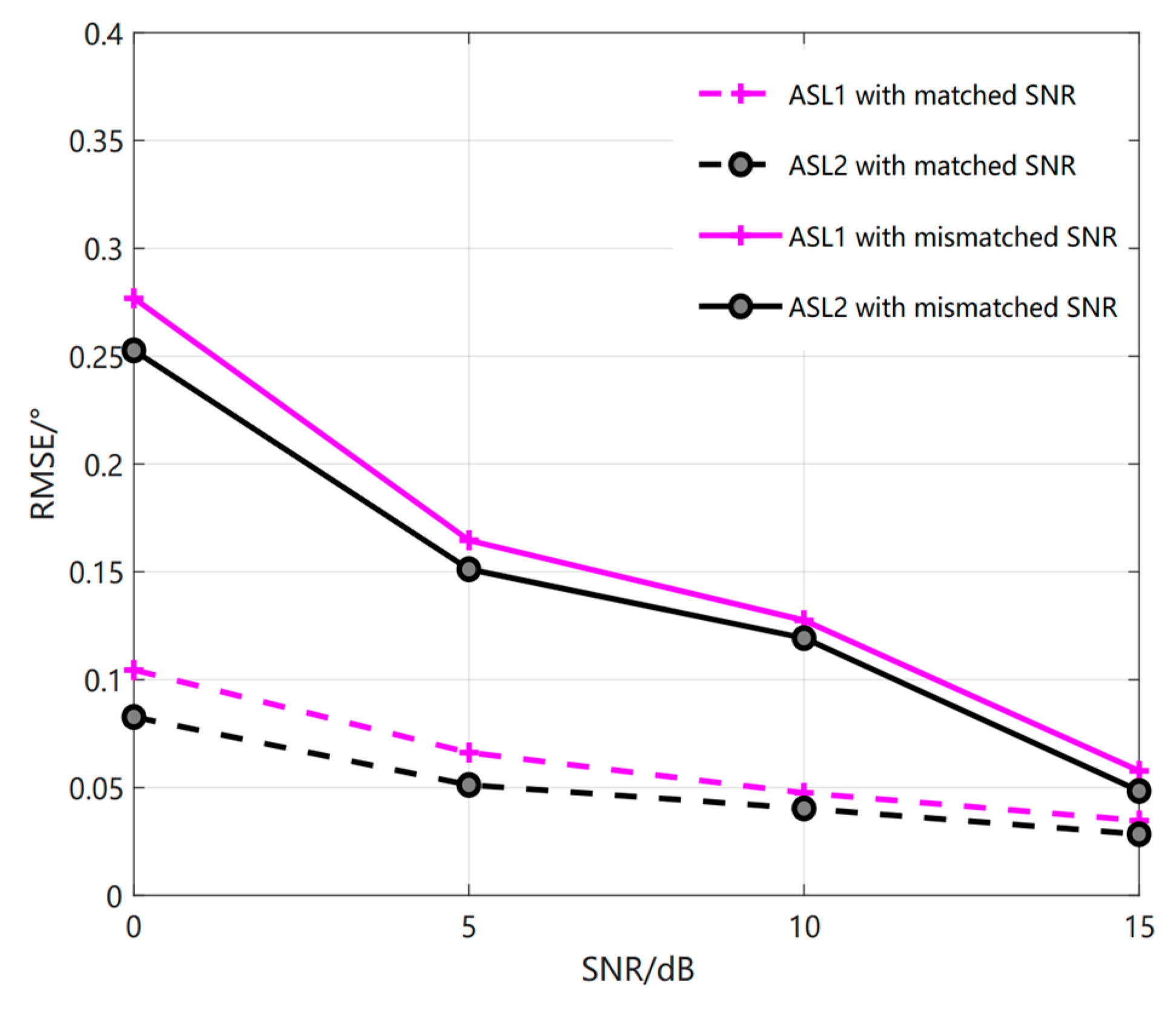
| ASL1 | 0.0642° | 0.0004 |
| ASL2 | 0.0513° | 0.0004 |
| S2S-MRL | 0.0372° | 0.0007 |
Disclaimer/Publisher’s Note: The statements, opinions and data contained in all publications are solely those of the individual author(s) and contributor(s) and not of MDPI and/or the editor(s). MDPI and/or the editor(s) disclaim responsibility for any injury to people or property resulting from any ideas, methods, instructions or products referred to in the content. |
© 2023 by the authors. Licensee MDPI, Basel, Switzerland. This article is an open access article distributed under the terms and conditions of the Creative Commons Attribution (CC BY) license (https://creativecommons.org/licenses/by/4.0/).
Share and Cite
Wu, Z.; Wang, J. Small Sample Coherent DOA Estimation Method Based on S2S Neural Network Meta Reinforcement Learning. Sensors 2023, 23, 1546. https://doi.org/10.3390/s23031546
Wu Z, Wang J. Small Sample Coherent DOA Estimation Method Based on S2S Neural Network Meta Reinforcement Learning. Sensors. 2023; 23(3):1546. https://doi.org/10.3390/s23031546
Chicago/Turabian StyleWu, Zihan, and Jun Wang. 2023. "Small Sample Coherent DOA Estimation Method Based on S2S Neural Network Meta Reinforcement Learning" Sensors 23, no. 3: 1546. https://doi.org/10.3390/s23031546
APA StyleWu, Z., & Wang, J. (2023). Small Sample Coherent DOA Estimation Method Based on S2S Neural Network Meta Reinforcement Learning. Sensors, 23(3), 1546. https://doi.org/10.3390/s23031546