Abstract
Nowadays, state-of-the-art direct visual odometry (VO) methods essentially rely on points to estimate the pose of the camera and reconstruct the environment. Direct Sparse Odometry (DSO) became the standard technique and many approaches have been developed from it. However, only recently, two monocular plane-based DSOs have been presented. The first one uses a learning-based plane estimator to generate coarse planes as input for optimization. When these coarse estimates are too far from the minimum, the optimization may fail. Thus, the entire system result is dependent on the quality of the plane predictions and restricted to the training data domain. The second one only detects planes in vertical and horizontal orientation as being more adequate to structured environments. To the best of our knowledge, we propose the first Stereo Plane-based VO inspired by the DSO framework. Differing from the above-mentioned methods, our approach purely uses planes as features in the sliding window optimization and uses a dual quaternion as pose parameterization. The conducted experiments showed that our method presents a similar performance to Stereo DSO, a point-based approach.
1. Introduction
A requirement for a mobile robot’s autonomy is the ability to extract useful information from the environment and create a map by using its sensors, while the robot explores the environment and simultaneously locates itself with that map. The research areas that address this problem using cameras as the main sensor are called Visual Odometry (VO) and visual Simultaneous Localization and Mapping (vSLAM).
According to Chen et al. [1], these techniques can be classified into two main different approaches: feature-based or direct techniques. The first is based on the extraction of features present in successive images to, through correspondence between these features, determine the pose of the robot and reconstruct a sparse map. The second approach minimizes the photometric error between a set of pixels of two images using a homography function. Both techniques are used in either monocular, stereo or RGB-D camera systems.
While early works paid more attention to the quality of pose estimates, with the extraction of sparse environment information, recent works have focused on improving the quality and density of the mapping in the SLAM process. More accurate sensors, computer processing power increase and new techniques contributed to the emergence of (semi-)dense and/or large-scale maps in VO and visual SLAM systems [2]. Now, some techniques allow choosing the density of the map according to the computational resources available [3].
These maps can be constructed with many types of features present in the environment, starting from geometric primitives, such as points [4], lines [5] and planes [6], to more complex structures, for instance, quadrics [7], cubics [8] and objects detected via Convolutional Neural Networks (CNNs) [9].
A predominance of techniques based on keyframes is observed in direct methods [10,11], which in general store point information in certain frames along a path traveled by the robot. Thus, point-based maps are widely used in such techniques. One of the reasons for this is the fact that high-gradient regions are present in corners and edges, which can be used to obtain disparity maps and create point-based maps. However, the use of points for map representation could be computationally expensive as far as the number of points increases and they do not contribute to the overall interpretation of the 3D structure of the mapped environment since each point is represented independently.
A more appropriate map representation, when the desired requirement is to use features that optimize the relationship between density and stored information, is to make use of planar regions. Planes are dominant in structured environments, both internal and external, and can be expandable, representing a large part of the scene with a few parameters [7]. Planes make possible the use of some constraints, such as Manhattan constraints [6,7], to restrict the relationship between planes in the environment, producing more consistent maps. Furthermore, it is possible to assign semantics to planar regions, since a region can represent, for example, walls or the floor and a set of planar regions can represent more complex structures [12].
The most prominent direct VO approach in recent years was developed by Engel et al. [10], called Direct Sparse Odometry (DSO). This technique initially developed for monocular cameras is based on point cloud and has become popular due to the quality of the results obtained in estimating odometry with reduced information. Several works have been developed from this technique. However, only recently, works developed by Wu and Beltrame [13] and Xu et al. [14] presented the first methods that use planes within the DSO framework.
In the first mentioned planar technique, the inverse depth of a pixel, used as the feature parameter in the DSO method, is expressed as a function of the homogeneous plane variables. This plane representation can also be understood as the coefficients of a unit quaternion [15]. Although this technique presents a valid description of the use of planes in the DSO framework, it requires that sufficiently good initial estimates of planes be obtained for the optimization to converge. To solve this problem, this technique made use of a plane estimator based on a CNN, which restricts the whole approach to the data domain used to train the network. In addition, it causes the method to depend on the quality of network predictions to initialize properly.
The second mentioned planar technique uses points that are part of the same plane to add a constraint to the optimization and increase the accuracy of the odometry results. This technique prioritizes indoor environments as far as it detects vertical and horizontal planes.
A representation of planes that is also minimal and follows the natural evolution of the DSO approach is the inverse depth of three image points [16]. The use of this approach makes possible the employment of disparity-based algorithms, which estimate point depth, already used by DSO. Furthermore, this approach causes the map features to be interpreted in two ways, i.e., as a set of three points or as a planar region formed by three vertices. This dual interpretation can be advantageous in situations in which point segmentation algorithms in image planes fail, causing points from different planes to be present in the same segment.
Thus, inspired by the DSO approach, the goal of this paper is to present a purely direct stereo VO framework that performs mapping with planar regions, represented by three-point inverse depths.
The proposed framework is, to the best of our knowledge, the first stereo plane-based VO inspired by the DSO framework. Moreover, we first introduce the use of dual quaternions in parameterizing the robot pose for direct methods. According to Wang et al. [17], among the various existing rigid body representations, the unit dual quaternion offers the most compact and computationally efficient screw transformation formalism.
This paper is organized as follows. Section 2 is a literature review of the main works in the area of direct VO and visual SLAM. In Section 3, a brief introduction of the main theoretical components addressed in this paper is presented. Then, Section 4 presents the Direct Planar Odometry framework. Section 5 presents the results of the proposed technique, as well as a discussion about them. Finally, in Section 6, we highlight the main ideas and contributions of this work and present some prospects for future works.
2. Related Works
This section presents a literature review of the developed techniques of Direct VO and visual SLAM. These techniques are classified according to the generated map as point-based or plane-based. Subsequently, SLAM methods that use dual quaternions for pose parameterization are presented. Finally, the main contributions of this paper are listed.
2.1. Point-Based Direct VO/SLAM
One of the most popular approaches has been the technique developed for monocular cameras called Large-Scale Direct SLAM (LSD-SLAM) [18]. LSD-SLAM presents a direct SLAM framework that generates a consistent large-scale map. For this, a semi-dense depth map, obtained from high-gradient pixels, is used in the image alignment. In the pose parameterization, the Lie group SIM(3) is applied and in addition to the rigid body parameters (rotation and translation), a scale parameter is added. Finally, this method achieves a consistent global map formed by 3D points through pose-graph optimization. A stereo camera version [11] and an extension of it [19], as well as an omnidirectional camera approach [20], have also been developed.
Recognizing some deficiencies in LSD-SLAM, mainly in pose estimation, some researchers have proposed improvements to the framework. Wang et al. [21] proposed to improve the initial estimation of VO by incorporating a constant-velocity model to provide initial estimates for the optimization, whereas Zhang et al. [22] developed a learning-based confidence model, which applied to the depth map helps in choosing the best pixels to be used in the optimization.
Later, the same research group that developed LSD-SLAM proposed DSO, which brought significant improvements in monocular odometry by optimizing camera poses, intrinsic and map parameters, boosting results through the use of photometric camera calibration. Subsequently, several versions of this work were presented, mainly addressing the use of different camera types [3,23], a modification with loop closure [24] and using predictions provided by deep learning techniques [25]. Yang et al. [26] proposed a semi-supervised network called StackNet for deep monocular depth estimation; these estimates were incorporated to overcome scale drift, an intrinsic limitation in monocular VO. The so-called Deep Virtual Stereo Odometry (DVSO) framework incorporates the left disparity prediction in the depth initialization and the right prediction in the bundle adjustment process using a virtual stereo term. More recently, Yang et al. [27] developed the D3VO, which integrated three pieces of information predicted by a semi-supervised network to benefit a monocular odometry method. More specifically, they used a network based on MonoDepth2 [28] which, besides predicting depth and relative camera pose, also retrieves photometric uncertainty and brightness transformation parameters. These predictions were then used through the processing framework, respectively, serving as initial values for both the front-end tracking and back-end optimization, performing inter-frame illumination alignment and weighting the photometric residuals.
Other approaches based on the DSO technique have also been developed. One of these approaches was SalientDSO [29] which, inspired by human vision, searches for regions of interest in the image that serves as input to the system. Parallelization of the original approach was proposed by Pereira et al. [30]. In addition, semi-direct approaches that mix direct VO methods and indirect ones to refine keyframe pose are also present in the literature [31,32,33].
2.2. Plane-Based Direct SLAM
One of the first real-time direct SLAM techniques to gain notoriety was the work proposed by Silveira et al. [16], who developed a monocular SLAM, using planes to generate the map, optimized by Efficient Second-order Minimization (ESM). To obtain initial estimates of the parameters, an approach that couples the proposed direct technique with a filter-based method was adopted.
Plane parameterization using the depths of three points, represented by three non-collinear pixels in a given image patch, is also introduced in the mentioned approach. This representation was employed on several square-shaped patches, subdividing the image, to estimate the plane parameters. In some situations in which patches are projections of regions with more than one plane in the scene, not necessarily all pixels of the patch will be contained in the same plane as the three points used in the parameterization. Such pixels can affect the correct estimation of the parameters.
In the approach DPPTAM [34], a monocular technique based on LSD-SLAM is developed using a semi-dense depth map. In the mentioned paper, the image is segmented using superpixels [35] and the points of the semi-dense map are projected onto the image and clustered according to plane parameterization segmentation performed by the superpixels. After that, the planes are estimated using Singular Value Decomposition (SVD) applied to the points clustered in each superpixel. DPPTAM keeps the points of a superpixel, allowing the use of non-convex regions. However, this is not a compact representation, since all the points of the superpixel are stored. In other words, the same problem of point-based visual SLAM techniques remains.
Ma et al. [36] developed CPA-SLAM, a real-time visual SLAM technique developed for RGB-D cameras that mix photometric and geometric alignment in the same optimization. To estimate planes, the keyframe is segmented into many regions and a global plane model that uses graph optimization is applied in all local observations.
As mentioned previously, the recent work by Wu and Beltrame [13] presented the first planar DSO-based technique. For each point chosen at each new image, parameters of the plane represented by unit quaternions are estimated. When a set of neighboring points projected from different keyframes in the current frame have the same descriptor, a planar region is determined and inserted into the optimization. The prediction strategy is performed using the PlaneNet [37] technique, which estimates the planes present in each pixel from a color image. This CNN-based technique is time-consuming and its efficiency depends on the domain of the network training data, which in practice limits the applicability of the framework as a whole.
The second planar DSO-based approach (PVI-DSO) is presented by Xu et al. [14], who developed a visual-inertial odometry (VIO) technique that fuses coplanar constraint regularities to improve the accuracy of the localization. In this application, only vertical and horizontal planes are detected, prioritizing its use in structured environments.
All approaches mentioned above showed a preference for point-based maps in direct SLAM applications. Among the few direct techniques found that use planes, none of them is a stereo-based framework.
2.3. Pose Parameterization
Different parameterizations for the pose have been used in visual SLAM and VO techniques. The homogeneous transformation matrix alongside its algebra has been one of the preferred approaches of the main direct SLAM methods. Virtually all of the techniques presented in this paper use this approach or a similar one, such as , which takes into account the scale factor.
One parameterization that is not new but that has recently been employed in visual SLAM techniques is unit dual quaternion. According to Thomas [38], quaternions are of vital importance in representing spatial rotations; however, a lack of precise understanding of the meaning of its operations leads to an underutilization of quaternion-derived techniques, such as dual quaternions.
According to Kenwright [39], dual quaternions are compact, unambiguous, singularity-free and computationally minimalist for rigid transformations. In addition, they offer the most compact way to represent rotations and translations. More recently, they have been employed in visual SLAM techniques based on stochastic filters [40,41,42,43,44,45], and some based on graph-SLAM [46,47] have been observed. Despite the wide use of this parametrization in feature-based SLAM approaches, our approach is the first to use it in direct VO.
2.4. Contributions
The main contribution of this work is the development of a plane-based direct VO technique inspired by the DSO approach. To the best of our knowledge, our work is the first purely direct stereo VO approach to use planes as features. The proposed plane parameterization represents a natural evolution of the DSO technique and has the following qualities:
- From the pose optimization point of view, the vertices of the planar region do not need to be part of the same real scene plane. For these cases, it is possible to interpret the feature as a set of three points. Thus, there is no need for differentiation of points and planes in the mathematical formulation of the problem.
- As a consequence of the previous statement, this parameterization allows the use of fast but low accuracy, algorithms for segmenting pixels into planes, not hindering the performance of the technique as a whole.
- Inspired by the DSO technique, which uses only a set of 8 pixels per point in the parameter optimization, this work uses only 8 pixels per vertex of the planar region, which represents only 24 pixels per plane. Depending on the distance between vertices, it can describe a large planar area in the scene with a small amount of data.
- This approach allows the three vertices of an existing planar region to be reused to form new planar regions, even contributing to a better coupling between the map elements.
A second contribution is the use of dual quaternion for representing the pose, that being the first direct VO technique that uses this type of parameterization.
3. Theoretical Background
In this section, the basic concepts for the development of this work are presented, starting with the homography model, which is dependent on the camera pose and the planes in the environment. Then, the basic concepts of the unit dual quaternion, the plane parameterization and the efficient second-order optimization model are presented. Some of these topics have been presented in a previous study by the authors, which compares different parameterizations of a plane [48]. However, for didactic purposes, we decided to present these concepts again in this article.
3.1. Plane-Based Two-View Homography
Figure 1 shows the projections of point , belonging to the plane , on the reference image and the image . It is assumed that the projections and , where is a identity matrix, is the intrinsic parameters matrix, is the rotation matrix and is the translation vector. The equation that maps to is given by:
where is the inverse depth of the point , relative to the reference frame and, in this case, ∝ means an up-to-scale equality.
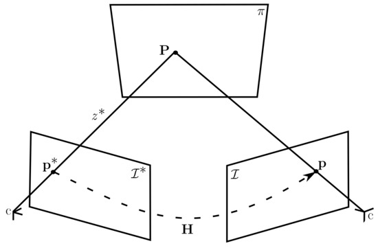
Figure 1.
Homography between two images given a plane.
The relationship between the plane and the inverse depth is given by:
where plane is parameterized by the unit normal vector and its distance from the reference frame. Thus, substituting in Equation (1) by Equation (2), we find:
such that and is the homography matrix. Finally, multiplication between and leads to:
where means homography matrix element.
The parameters of the homography matrix are , representing plane information, and , representing a pose. Since the front-end of this work estimates pose and plane parameters separately, the optimization formulation of the plane and pose will be presented independently.
For plane estimation, the pose between two images is considered to be known. This relative pose can be static, i.e., given by the stereo baseline, and temporal, given by successive images of the left camera. Thus, Equation (3) becomes:
In the step for obtaining the relative pose of subsequent images from the left camera, the structure information is considered known and Equation (3) becomes:
3.2. Problem Formulation
In contrast to the DSO approach, the optimization technique used to estimate planes and poses in this work is Efficient Second-order Minimization (ESM). This second-order technique, presented by Malis [49], has as its main advantage the need to determine only first-order approximations.
The photometric error is formulated as a non-linear optimization problem and it is defined as:
where represents pose parameters and represents plane parameters.
3.2.1. Plane Optimization
The plane is estimated by the optimization considering the relative pose between a given frame and a reference frame is known. Therefore, Equation (7) is rewritten to include only as parameter in the optimization:
where the photometric error element is part of the residual vector of size () and represents the vector of parameters of , such that:
where is the function that maps the parameter vector of the plane to its normal representation , applied in Equation (3).
Similar to other optimization methods (e.g., Newton), ESM is an iterative method. To determine the new estimate , a function dependent on the previous estimate and the increment is applied:
where represents the theta update function, which depends on the relation between and . The optimization will estimate new values of until the established stopping criterion is satisfied.
On the assumption that is expanded in a second-order Taylor series around the point , we have:
where and are the Jacobian and Hessian evaluated at and , respectively.
As a central feature of the ESM method, in Equation (11) the Hessian matrix must be expressed in terms of Jacobian. To enable this, the Jacobian is expanded in a first-order Taylor series and we obtain:
Thus, by substituting in Equation (11) with Equation (12) and dropping the second- and third-order residuals, we have:
Applying the optimization condition from Equation (8) and solving it, we find:
where is the optimal increment that satisfies the optimization criterion.
Applying the same simplifications adopted by Silveira et al. [16], we assume that . Thus, Equation (14) becomes:
where , is the photometric error vector with all pixels applied in the optimization, and are the image gradient of the reference and current frames and is the matrix demonstrated by Benhimane and Malis [50]. is the Jacobian of relative to the parameters of .
Finally, the increment of is given by:
3.2.2. Plane Parameterization
There are several ways to parameterize a plane and the chosen parameterization influences the efficiency of the optimization. Following Lins et al. [48], the parameterization applied in this work uses the inverse depth information of three non-collinear pixels belonging to the reference image (Figure 2). Considering that these three points are in the same plane, the vector is defined as:
where , and are the depth of these points.
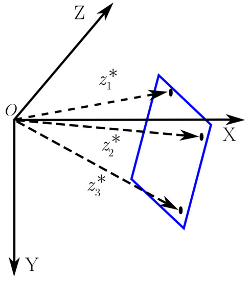
Figure 2.
The figure shows three non-collinear points, belonging to the plane and projected onto the reference image with depths , and , respectively.
For this parameterization, as introduced by Equation (9), the function which maps the parameters to is given by:
where:
are the pixel coordinates, in the reference image, of the three points and is the matrix of intrinsic parameters. The update rule, given by function (Equation 10) is:
3.2.3. Pose Optimization
The problem of estimating the pose parameters is solved in the same way as plane optimization. In this case, Equation (7) becomes:
where represents the homogeneous transformation matrix belonging to the Lie group of rigid transformations. Similarly, the goal of this step is to find the unit dual quaternion , which represents pose parameters and such that the reprojection error is minimal.
Using ESM, we find a similar result to that obtained in the plane optimization, given by:
where represents the Jacobian of pose and the vector is the reprojection error. Finally, the pose increment is given by:
3.2.4. Unit Quaternion
Quaternions were introduced by Hamilton in 1866 as an extension of the complex number theory to formulate a four-dimensional manifold [38]. A quaternion is a four-component number consisting of a scalar part and a vector part . Formally, a general quaternion q is defined as:
where its conjugate is given by . The vector form is and the orthogonal complex numbers , and are defined, such that .
The addition of two quaternions and is and the product of two quaternions is given by the Hamilton product, where:
When the scalar part is equal to zero, the quaternion is written as and is called a pure quaternion. Since is a three-dimensional vector, clearly there is a one-to-one correspondence between vectors in 3D space. In addition, a quaternion with a unit length, where , is called a unit quaternion and can be used to represent rotation about an axis (denoted by the unit vector ) and an angle as follows:
3.3. Unit Dual Quaternion
A dual quaternion, denoted by , is defined as a dual number comprised of two quaternion components:
where and are quaternions representing the real and dual parts, and denotes the dual unit, which is defined by and . Equivalently, the dual quaternions can be defined as an eight-dimensional vector space:
where the first four elements represent the real part and the last four elements represent the dual part. The unit dual quaternion is subject to the constraint , where is its conjugate.
As the unit quaternions can be used to represent rotations, the unit dual quaternions can be used to represent rigid transformation [39]. Thus, the real part of the unit dual quaternion is a unit quaternion that represents rotation and the dual part represents translation combined with rotation:
and
where is a pure quaternion formed with position vector.
To link the unit dual quaternions with optimization, the homogeneous transformation matrix is given in terms of the unit dual quaternion:
and the update rule used in optimization is given by:
where the updated pose is obtained by the multiplication of the pose and the optimization increment through the Hamilton product.
3.4. Summary of DSO
DSO is a keyframe-based approach, in which each keyframe is responsible for storing several high-gradient points, distributed over the image. Using a sliding window procedure, only a fixed amount of keyframes are kept in the system. Whenever a new keyframe needs to be created, an old keyframe is discarded. Each point of each keyframe has its inverse depth estimated through disparity, refined through Gauss–Newton optimization and kept in a semi-dense depth map.
A total of 2000 points, distributed along the keyframes belonging to the sliding window, are chosen and called active points. Whenever a new frame is available, these points are used to estimate the new pose. Later, the active points are used in the sliding window optimization, which is responsible for refining the pose estimates of all the keyframes of the sliding window and the depth parameters of the active points. In the global optimization, the intrinsic camera parameters and the affine brightness correction factors are also refined.
The energy function used in DSO is given by Equation (35):
where can be found by Equation (1), , , a, b are the brightness parameters of the reference and current images and is a gradient-dependent weighting factor. consists of the set including all pixels in the optimization. represents the Huber norm.
As active points leave the scene or become occluded, they are marginalized and other points are activated. When many points of a single keyframe are discarded, the entire keyframe is marginalized and a new keyframe is inserted into the sliding window.
4. Direct Planar Odometry (DPO) with Stereo Camera
The proposed framework is based on DSO and is organized according to Figure 3. The system is divided into two parts: front-end and back-end. The front-end is composed of the system initialization, the tracking step and the creation and deletion of keyframes from the sliding window. The back-end is responsible for optimizing all the parameters belonging to the sliding window keyframes.
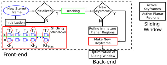
Figure 3.
Framework of the proposed approach.
In the system startup, the first stereo pair is detected and a set of high-gradient pixels, distributed over the entire left image of the stereo pair, is selected. The inverse depth of each pixel is estimated through disparity and refined through optimization. Some of these points are used for planar region creation, which will be part of the first keyframe of the sliding window.
When the second stereo pair is available, the tracking algorithm estimates the relative pose between the keyframe and the current frame. Then, through a set of rules, the system checks if it is necessary to turn the current frame into a new keyframe. If so, points from the current frame are selected to form new immature planes, which are a set of planes from which the active planes are selected, i.e., the planes that will be part of the optimization. Moreover, whenever a new keyframe is created, the sliding window optimization is performed. Additionally, this step is also responsible for managing planar regions from a given keyframe inside the sliding window.
4.1. Initialization
The first step carried out in initialization is the selection and depth estimation of high-gradient points in the left image. The procedure for point and depth estimation is the same as in Stereo DSO [3]. These points are used to create planar regions in the image. This step is carried out by creating a set of triangles generated by the 2D Delaunay triangle algorithm. This routine differs from PVI-DSO [14], which uses 2D Delaunay triangulation over the DSO depth map.
Finally, the initialization is performed at different resolutions of the image (pyramid levels) and the estimated features are used in the tracking step. The planar regions generated at the original image resolution are activated and stored in the first frame, which is the first keyframe of the sliding window.
4.2. Tracking
As indicated in Figure 3, the tracking step is performed between the left camera images. Using the formulation presented in Equation (25), parameterized with unit dual quaternions (Section 3.3) and using planar regions, the relative pose between the current frame and the newest keyframe can be determined by the tracking algorithm. The active planes, applied in the tracking step of all keyframes in the sliding window, are projected in the newest keyframe. In addition, as in DSO, the constant motion model is used for estimating the initial pose and in optimization, an image pyramid approach is employed.
4.3. Keyframe Creation and Disposal
The creation and exclusion of new keyframes follow a similar rule to the one adopted in DSO [10]. Their work uses three criteria for creating a new keyframe: the optical flow mean squared error (MSE), the optical flow MSE without rotation and the relative brightness factor between two images. Since this work does not use brightness parameters, only the first two criteria are used to manage when new keyframes should be created.
In our approach, the management keyframe exclusion is effected with two criteria: the keyframe number of planar regions participating in the sliding window optimization and the keyframe age. Keyframes with fewer active planar regions and that are not among the two newest keyframes have priority to be discarded. Like the DSO, a limit of seven keyframes is defined to be kept in the sliding window.
4.4. Planar Region Creation and Disposal
In the DSO approach, when a new keyframe is inserted into the sliding window, a series of high-gradient points are selected from the left-image keyframe. Some of these selected points are observations of keyframe points, inside the sliding window. To prevent these points from being inserted in the newest keyframe, the DSO uses a distance map. It expresses the distances of map elements to points of all sliding window keyframes, projected onto the image of the newest keyframe. Thus, the system can discard points with the same image position as existing points.
In contrast, in the construction of the DPO map, only active planes are used, i.e., planar regions of all keyframes considered in the sliding window to participate in the optimization. As they are composed of three points, the vertices of these regions are projected onto the image of the newest keyframe with halved resolution. This resolution reduction procedure is equivalent to expanding the vertex size in the newest image. The position in the image of each projected vertex is used in the distance map, which has the same dimensions as the reduced image.
All elements of the distance map are initialized with the integer 1000, representing that still there are no nearby neighbor projected planes. Then, the indexes of the planar region vertices are used to attribute zero in the corresponding distance map elements, a value that indicates occupied positions. A rasterization process is also performed on each planar region to insert zero in the inner parts of these planes, indicating that these elements are also occupied positions.
To attribute values for other map elements, a point is chosen for each planar region edge. These points are defined by the intersection of the edge with the line formed by the region centroid and the remaining vertex, which is not part of the edge. From these points, elements neighboring an element that has a smaller integer number get the smaller number added to the number 1. Thus, this procedure allows the distance map to report the distance from an element of the array to an edge of a planar region.
Each time a new keyframe is created, high-gradient points distributed throughout the left image are selected. The depth of these points is estimated through disparity. Two-dimensional Delaunay triangularization is applied to these points to generate a set of triangles, which are considered immature planes whenever the depths of their vertices are valid.
Similar to DSO, part of these planes can be activated and included in the optimization, according to the maximum number of regions. To be activated, an immature plane cannot be an observation of another active plane. To achieve this, before a plan is activated, a check of its position with respect to other active points is performed using the distance map. Figure 4 shows an example of how new planar regions are created.
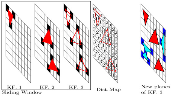
Figure 4.
The example shows a sliding window formed by two old keyframes and one new keyframe. In the first keyframe (KF. 1), there is an active planar region, represented by the triangle (red) and its vertices (black). The second keyframe (KF. 2) has two active planar regions. The third keyframe (KF. 3) shows projections of the vertices from the previous keyframes (black). The distance map is exemplified in the fourth frame. Elements with zero indicate occupied positions with old edges. Elements with values above zero represent the distance from the element to the edge. Thus, new planes that fall at a certain distance from the edges of old activated planes are accepted to be activated in the new keyframe. Finally, the last frame presents new activated planes (cyan) and their vertices (blue).
When the number of active planes is greater than the defined maximum number, the ones that leave the image or have a high residual are discarded. This procedure differs from the one performed with DSO. In their method, parameters from the keyframe that will be discarded are used one last time in the sliding window optimization.
4.5. Sliding Window Optimization
The optimization is performed with all active planes of all keyframes in the sliding window. When a given plane of an active keyframe is visible in another one, we consider this an observation. Thus, in this approach, an observation always takes place between two keyframes. In addition, since the sliding window keyframes have geometric proximity, a given planar region can have multiple observations.
The formulation of the sliding window optimization can be represented by:
where is the vector with all optimized parameters, is the vector of pose parameters, is the vector of feature parameters, represents the set of keyframes in the sliding window, is the set of active planar regions of a keyframe and is the number of observations of a given planar region .
Since the pose parameters of the stereo pair are fixed, the feature observations realized by the stereo pair are not directly added to the optimization. To take into account the information of these observations, we perform a similar procedure carried out with Stereo DSO. This procedure consists of replacing the residual of the temporal stereo observations with:
where is the weighted average of the static and temporal residuals, given that is a constant fixed in 0.15 and represents the relative pose between the keyframe k and the j-th observation.
The increment of the parameters is given by:
where represents the Jacobian matrices of the relative poses and active planar regions and represents the residual vector of all observations.
As the DSO, this formulation also uses the concept of First Estimate Jacobian [51] in the assembly of the Hessian matrix and Shur’s elimination; these are done similarly. In addition, in their method, the marginalized variables in Shur’s elimination are points that will be discarded. The proposed technique, on the other hand, marginalizes the active features in the same manner as is common in indirect methods [52]. Moreover, since the terms of the residuals in the optimization matrix depend on two frames, the adjoint dual unit quaternion is used to relate relative pose to absolute pose [53]. An example of a configuration of the sliding window can be viewed in Figure 5.
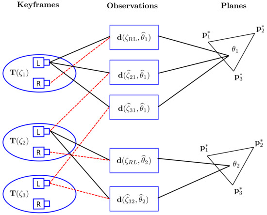
Figure 5.
The example shows a sliding window with three keyframes, with poses , and . There are two planar regions, belonging to the first keyframe, having three observations, and belonging to the second keyframe, having two observations.
5. Experimental Results
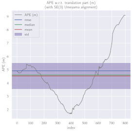
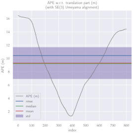
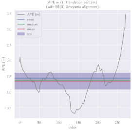
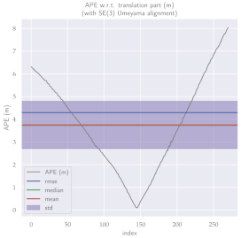
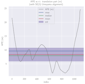
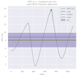
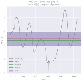
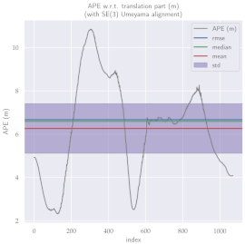
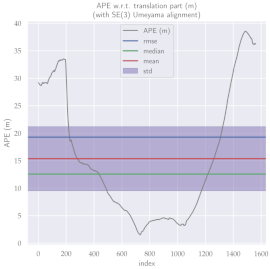
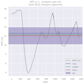
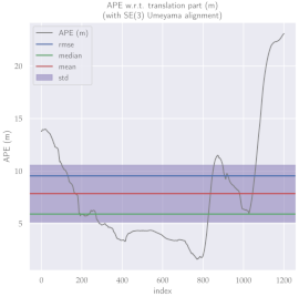
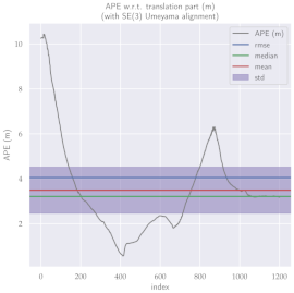
For performance evaluation and comparison of the method, six sequences from the KITTI dataset [54] were used. In each of these sequences, an average trajectory was used, defined by the average of ten simulations. As an evaluation criterion, the Absolute Pose Error (APE), implemented in Python’s EVO library [55], was used. This metric compares the reference poses (ground truth) with the poses estimated with the VO/SLAM method. For the simulations, whenever possible, we tried to use the same configuration parameters as the DSO in the DPO. Thus, parameters such as the number of pixels per point or vertex were set to eight (8) and the maximum number of active keyframes within the sliding window was seven (7). The results for each sequence can be viewed in Table 1, Table 2 and Table 3. For each sequence, the APE metric is given for each frame of the sequence. Information such as RMS error, mean, median and standard deviation are also presented.

Table 1.
The absolute pose error (APE) for all frames of sequences 3 and 4 of the KITTI dataset.

Table 2.
The absolute pose error (APE) for all frames of sequences 6 and 7 of the KITTI dataset.

Table 3.
The absolute pose error (APE) for all frames of sequences 9 and 10 of the KITTI dataset.
Discussion
Analyzing the graphs of sequences 3, 4, 6, 7, 9 and 10 from the KITTI dataset, it is possible to notice in Table 4 that in sequences 3, 4 and 7 the mean errors and standard deviations were smaller in the DPO. In sequences 6 and 9, DPO mean errors were slightly above the DSO. However, the maximum errors of the DPO were much larger than the DSO, indicating large errors at isolated points of the trajectory. Finally, sequence 10 showed a much smaller mean error and standard deviation for DSO. It is important to emphasize that even without photometric camera calibration and optimization of brightness parameters, the DPO presented a similar performance to the DSO and obtained better results in half of the evaluated cases. However, of the six analyzed sequences, three presented a much higher maximum error for DPO, a fact that might be partially justified by the lack of optimization of illumination parameters. In the future, we intend to insert an illumination optimization model into the proposed technique.

Table 4.
Comparison of mean error, standard deviation and minimum and maximum error of the six analyzed sequences between DPO and Stereo DSO.
From a computational cost point of view, we measure the frame per second (FPS) for both methods. Although DPO was programmed on the stereo DSO platform, no multi-threading parallelization or SSE (Streaming SIMD Extensions) instruction set was used to accelerate the algorithm. Nevertheless, on a 7th-generation Intel core-i5 PC with 8 GB RAM, the algorithm runs at a rate of about 1 FPS, while DSO runs at a rate of 5.63 FPS. Looking at the computational cost from the perspective of the amount of data used in the optimization, the number of active planes is limited to 667 planes in the sliding window. Since each plane consists of three points, the maximum number of points per optimization is 2001 points, equivalent to the number used by Stereo DSO.
Figure 6 presents an example of the map reconstructed by our method. From a set of points, the planes used in the optimization are estimated from the Delaunay triangularization. Although this approach is ideal for coupling vertices that belong to different planes, for the sake of simplicity, in this first version the generated planes were considered independent. From the map point of view, this work is seen as a first step in the development of a map that can be used not only for odometry but also to represent structures in the environment to aid trajectory planning. Although some of the planes determined by the method may not represent real-world planes, Delaunay triangularization allows non-planar regions to be approximated by planes.
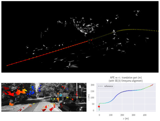
Figure 6.
This figure shows a sample result, taken from KITTI sequence 3. The bottom right image represents the resulting DPO trajectory. Sections with colors closer to blue indicate less positioning error. The star indicates the position of the keyframe, shown in the lower left image. Finally, the top image presents a sample 3D visualization of the map.
6. Conclusions
This paper presented a technique inspired by DSO, but instead of points, we make use of planar regions as features. It also introduced the use of dual quaternions to represent the camera’s poses in direct methods. Comparisons of the proposed technique with Stereo DSO were performed and the presented results showed DPO accuracy within the DSO standards, this being consistently superior in half of the experiments performed, given that each sequence was evaluated several times. In the future, in order to improve the accuracy of the odometry, we intend to add illumination parameters to the optimization, as well as loop closure detection. Moreover, in order to improve the map representation, we intend to make the features more susceptible to the inclusion of semantics, which could help in the trajectory generation.
Author Contributions
Conceptualization, F.C.A.L., A.A.D.M. and P.J.A.; methodology, F.C.A.L. and N.S.R.; software, F.C.A.L. and N.S.R.; validation, F.C.A.L. and N.S.R.; theoretical formulation, F.C.A.L.; writing—original draft preparation, F.C.A.L. and N.S.R.; writing—review and editing, F.C.A.L., N.S.R. and V.G.J.; supervision, P.J.A., A.A.D.M. and V.G.J. All authors have read and agreed to the published version of the manuscript.
Funding
This study was financed in part by the Coordination of Improvement of Higher Education Personnel—Brazil—CAPES (Finance Code 001, 23038.000776/2017-54 and 88887.123920/2014-00), by São Paulo Research Foundation—FAPESP (grant 2014/50851-0) and by the Brazilian National Council for Scientific and Technological Development—CNPq (grant 65755/2014-3).
Institutional Review Board Statement
Not applicable.
Informed Consent Statement
Not applicable.
Data Availability Statement
Not applicable.
Acknowledgments
We thank the Laboratory of Robotics and Dedicated Systems (LARS) at the Federal University of Rio Grande do Norte and the Laboratory of Intelligent Systems (LASI) at the University of São Paulo for providing materials and infrastructure to conduct the presented research.
Conflicts of Interest
The authors declare no conflict of interest.
References
- Chen, Y.; Zhou, Y.; Lv, Q.; Deveerasetty, K.K. A Review of V-SLAM*. In Proceedings of the IEEE International Conference on Information and Automation (ICIA), Wuyishan, China, 11–13 August 2018; pp. 603–608. [Google Scholar] [CrossRef]
- Newcombe, R.a.; Davison, A.J.; Izadi, S.; Kohli, P.; Hilliges, O.; Shotton, J.; Molyneaux, D.; Hodges, S.; Kim, D.; Fitzgibbon, A. KinectFusion: Real-time dense surface mapping and tracking. In Proceedings of the 10th IEEE International Symposium on Mixed and Augmented Reality (ISMAR), Basel, Switzerland, 26–29 October 2011; pp. 127–136. [Google Scholar] [CrossRef]
- Wang, R.; Schwörer, M.; Cremers, D. Stereo DSO: Large-Scale Direct Sparse Visual Odometry with Stereo Cameras. In Proceedings of the IEEE International Conference on Computer Vision (ICCV), Venice, Italy, 22–29 October 2017; pp. 3923–3931. [Google Scholar] [CrossRef]
- Mur-Artal, R.; Montiel, J.M.M.; Tardós, J.D. ORB-SLAM: A Versatile and Accurate Monocular SLAM System. IEEE Trans. Robot. 2015, 31, 1147–1163. [Google Scholar] [CrossRef]
- Pumarola, A.; Vakhitov, A.; Agudo, A.; Sanfeliu, A.; Moreno-Noguer, F. PL-SLAM: Real-time monocular visual SLAM with points and lines. In Proceedings of the IEEE International Conference on Robotics and Automation (ICRA), Singapore, 29 May–3 June 2017; pp. 4503–4508. [Google Scholar] [CrossRef]
- Le, P.H.; Kosecka, J. Dense piecewise planar RGB-D SLAM for indoor environments. In Proceedings of the IEEE International Conference on Intelligent Robots and Systems (IROS), Vancouver, BC, Canada, 24–28 September 2017; pp. 4944–4949. [Google Scholar] [CrossRef]
- Hosseinzadeh, M.; Latif, Y.; Pham, T.; Suenderhauf, N.; Reid, I. Structure Aware SLAM using Quadrics and Planes. In Computer Vision—ACCV 2018 Lecture Notes in Computer Science; Springer: Cham, Switzerland, 2018; Volume 11363, pp. 410–426. [Google Scholar] [CrossRef]
- Yang, S.; Scherer, S. CubeSLAM: Monocular 3-D Object SLAM. IEEE Trans. Robot. 2019, 35, 925–938. [Google Scholar] [CrossRef]
- Sharma, A.; Dong, W.; Kaess, M. Compositional Scalable Object SLAM. In Proceedings of the IEEE International Conference on Robotics and Automation (ICRA), Xi’an, China, 30 May–5 June 2021. [Google Scholar]
- Engel, J.; Koltun, V.; Cremers, D. Direct Sparse Odometry. IEEE Trans. Pattern Anal. Mach. Intell. 2018, 40, 611–625. [Google Scholar] [CrossRef] [PubMed]
- Engel, J.; Stückler, J.; Cremers, D. Large-scale direct SLAM with stereo cameras. In Proceedings of the IEEE/RSJ International Conference on Intelligent Robots and Systems (IROS), Hamburg, Germany, 28 September–2 October 2015; pp. 1935–1942. [Google Scholar] [CrossRef]
- Yang, S.; Song, Y.; Kaess, M.; Scherer, S. Pop-up slam: Semantic monocular plane slam for low-texture environments. In Proceedings of the IEEE/RSJ International Conference on Intelligent Robots and Systems (IROS), Daejeon, Republic of Korea, 9–14 October 2016; pp. 1222–1229. [Google Scholar]
- Wu, F.; Beltrame, G. Direct Sparse Odometry with Planes. IEEE Robot. Autom. Lett. 2022, 7, 557–564. [Google Scholar] [CrossRef]
- Xu, B.; Li, X.; Li, J.; Yuen, C.; Dai, J.; Gong, Y. PVI-DSO: Leveraging Planar Regularities for Direct Sparse Visual-Inertial Odometry. arXiv 2022, arXiv:2204.02635. [Google Scholar]
- Kaess, M. Simultaneous localization and mapping with infinite planes. In Proceedings of the IEEE International Conference on Robotics and Automation (ICRA), Seattle, WA, USA, 26–30 May 2015; pp. 4605–4611. [Google Scholar] [CrossRef]
- Silveira, G.; Malis, E.; Rives, P. An efficient direct approach to visual SLAM. IEEE Trans. Robot. 2008, 24, 969–979. [Google Scholar] [CrossRef]
- Wang, X.; Han, D.; Yu, C.; Zheng, Z. The geometric structure of unit dual quaternion with application in kinematic control. J. Math. Anal. Appl. 2012, 389, 1352–1364. [Google Scholar] [CrossRef]
- Engel, J.; Schöps, T.; Cremers, D. LSD-SLAM: Large-Scale Direct Monocular SLAM. In Computer Vision—ECCV 2014; Fleet, D., Pajdla, T., Schiele, B., Tuytelaars, T., Eds.; Springer International Publishing: Cham, Switzerland, 2014; pp. 834–849. [Google Scholar]
- Usenko, V.; Engel, J.; Stückler, J.; Cremers, D. Reconstructing Street-Scenes in Real-Time from a Driving Car. In Proceedings of the International Conference on 3D Vision (3DV), Lyon, France, 19–22 October 2015; pp. 607–614. [Google Scholar] [CrossRef]
- Caruso, D.; Engel, J.; Cremers, D. Large-scale direct SLAM for omnidirectional cameras. In Proceedings of the IEEE/RSJ International Conference on Intelligent Robots and Systems (IROS), Hamburg, Germany, 28 September–2 October 2015; pp. 141–148. [Google Scholar] [CrossRef]
- Wang, P.; Gao, C.; Guo, W.; Li, M.; Zha, F.; Cong, Y. Robust and fast mapping based on direct methods. In Proceedings of the 2nd International Conference on Advanced Robotics and Mechatronics (ICARM), Hefei and Tai’an, China, 27–31 August 2017; pp. 592–595. [Google Scholar] [CrossRef]
- Zhang, W.; Yan, Z.; Xiao, G.; Feng, A.; Zuo, W. Real-Time Direct Monocular SLAM With Learning-Based Confidence Estimation. IEEE Access 2019, 7, 103365–103376. [Google Scholar] [CrossRef]
- Matsuki, H.; von Stumberg, L.; Usenko, V.; Stuckler, J.; Cremers, D. Omnidirectional DSO: Direct Sparse Odometry With Fisheye Cameras. IEEE Robot. Autom. Lett. 2018, 3, 3693–3700. [Google Scholar] [CrossRef]
- Gao, X.; Wang, R.; Demmel, N.; Cremers, D. LDSO: Direct Sparse Odometry with Loop Closure. In Proceedings of the IEEE/RSJ International Conference on Intelligent Robots and Systems (IROS), Madrid, Spain, 1–5 October 2018; pp. 2198–2204. [Google Scholar] [CrossRef]
- Zhao, C.; Tang, Y.; Sun, Q.; Vasilakos, A.V. Deep Direct Visual Odometry. IEEE Trans. Intell. Transp. Syst. 2021, 23, 7733–7742. [Google Scholar] [CrossRef]
- Yang, N.; Wang, R.; Stuckler, J.; Cremers, D. Deep virtual stereo odometry: Leveraging deep depth prediction for monocular direct sparse odometry. In Proceedings of the 15th European Conference on Computer Vision (ECCV), Munich, Germany, 8–14 September 2018; pp. 817–833. [Google Scholar]
- Yang, N.; Stumberg, L.v.; Wang, R.; Cremers, D. D3vo: Deep depth, deep pose and deep uncertainty for monocular visual odometry. In Proceedings of the IEEE/CVF Conference on Computer Vision and Pattern Recognition (CVPR), Virtual, 14–19 June 2020; pp. 1281–1292. [Google Scholar]
- Godard, C.; Mac Aodha, O.; Firman, M.; Brostow, G.J. Digging into self-supervised monocular depth estimation. In Proceedings of the IEEE/CVF International Conference on Computer Vision (ICCV), Seoul, Republic of Korea, 27 October–2 November 2019; pp. 3828–3838. [Google Scholar]
- Liang, H.J.; Sanket, N.J.; Fermüller, C.; Aloimonos, Y. SalientDSO: Bringing Attention to Direct Sparse Odometry. arXiv 2018, arXiv:1803.00127. [Google Scholar]
- Pereira, C.; Falcao, G.; Alexandre, L.A. Pragma-Oriented Parallelization of the Direct Sparse Odometry SLAM Algorithm. In Proceedings of the 27th Euromicro International Conference on Parallel, Distributed and Network-Based Processing (PDP), Pavia, Italy, 13–15 February 2019; pp. 252–259. [Google Scholar] [CrossRef]
- Lee, S.H.; Civera, J. Loosely-Coupled Semi-Direct Monocular SLAM. IEEE Robot. Autom. Lett. 2019, 4, 399–406. [Google Scholar] [CrossRef]
- Tang, F.; Li, H.; Wu, Y. FMD Stereo SLAM: Fusing MVG and Direct Formulation Towards Accurate and Fast Stereo SLAM. In Proceedings of the International Conference on Robotics and Automation (ICRA), Montreal, QC, Canada, 20–24 May 2019; pp. 133–139. [Google Scholar] [CrossRef]
- Liang, W.; He, L.P.; Liu, J.; Wang, Y. A Robust RGB-D SLAM with Loosely-Coupled Semi-Direct Method. In Proceedings of the Global Reliability and Prognostics and Health Management (PHM-Shanghai), Shanghai, China, 16–18 October 2020; pp. 1–5. [Google Scholar] [CrossRef]
- Concha, A.; Civera, J. DPPTAM: Dense piecewise planar tracking and mapping from a monocular sequence. In Proceedings of the IEEE/RSJ International Conference on Intelligent Robots and Systems (IROS), Hamburg, Germany, 28 September–2 October 2015; pp. 5686–5693. [Google Scholar] [CrossRef]
- Achanta, R.; Shaji, A.; Smith, K.; Lucchi, A.; Fua, P.; Süsstrunk, S. SLIC Superpixels Compared to State-of-the-Art Superpixel Methods. IEEE Trans. Pattern Anal. Mach. Intell. 2012, 34, 2274–2282. [Google Scholar] [CrossRef] [PubMed]
- Ma, L.; Kerl, C.; Stückler, J.; Cremers, D. CPA-SLAM: Consistent plane-model alignment for direct RGB-D SLAM. In Proceedings of the IEEE International Conference on Robotics and Automation (ICRA), Stockholm, Sweden, 16–21 May 2016; pp. 1285–1291. [Google Scholar] [CrossRef]
- Liu, C.; Yang, J.; Ceylan, D.; Yumer, E.; Furukawa, Y. PlaneNet: Piece-Wise Planar Reconstruction from a Single RGB Image. In Proceedings of the IEEE/CVF Conference on Computer Vision and Pattern Recognition (CVPR), Salt Lake City, UT, USA, 18–23 June 2018; pp. 2579–2588. [Google Scholar] [CrossRef]
- Thomas, F. Approaching Dual Quaternions From Matrix Algebra. IEEE Trans. Robot. 2014, 30, 1037–1048. [Google Scholar] [CrossRef]
- Kenwright, B. A Beginners Guide to Dual-Quaternions: What They Are, How They Work, and How to Use Them for 3D. In Proceedings of the 20th International Conference on Computer Graphics, Visualization and Computer Vision (WSCG), Plzen, Czech Republic, 25–28 June 2012; pp. 1–13. [Google Scholar]
- Filipe, N.; Kontitsis, M.; Tsiotras, P. Extended Kalman Filter for spacecraft pose estimation using dual quaternions. In Proceedings of the American Control Conference (ACC), Chicago, IL, USA, 01–03 July 2015; pp. 3187–3192. [Google Scholar] [CrossRef]
- Sveier, A.; Myhre, T.A.; Egeland, O. Pose Estimation with Dual Quaternions and Iterative Closest Point. In Proceedings of the Annual American Control Conference (ACC), Milwaukee, WI, USA, 27–29 June 2018; pp. 1913–1920. [Google Scholar] [CrossRef]
- Varghese, A.; Chandra, M.G.; Kumar, K. Dual quaternion based IMU and vision fusion framework for mobile augmented reality. In Proceedings of the 9th IEEE International Symposium on Intelligent Signal Processing (WISP), Siena, Italy, 15–17 May 2015; pp. 1–6. [Google Scholar] [CrossRef]
- Bultmann, S.; Li, K.; Hanebeck, U.D. Stereo Visual SLAM Based on Unscented Dual Quaternion Filtering. In Proceedings of the 22th International Conference on Information Fusion (FUSION), Ottawa, ON, Canada, 2–5 July 2019; pp. 1–8. [Google Scholar]
- Sveier, A.; Egeland, O. Dual Quaternion Particle Filtering for Pose Estimation. IEEE Trans. Control. Syst. Technol. 2020, 29, 2012–2025. [Google Scholar] [CrossRef]
- Li, K.; Pfaff, F.; Hanebeck, U.D. Unscented Dual Quaternion Particle Filter for SE(3) Estimation. IEEE Control Syst. Lett. 2021, 5, 647–652. [Google Scholar] [CrossRef]
- Kim, J.; Cheng, J.; Shim, H. Efficient Graph-SLAM optimization using unit dual-quaternions. In Proceedings of the 12th International Conference on Ubiquitous Robots and Ambient Intelligence (URAI), Goyangi, Republic of Korea, 28–30 October 2015; pp. 34–39. [Google Scholar] [CrossRef]
- Cheng, J.; Kim, J.; Jiang, Z.; Che, W. Dual Quaternion-Based Graphical SLAM. Robot. Auton. Syst. 2016, 77, 15–24. [Google Scholar] [CrossRef]
- Lins, F.C.A.; Luz, O.M.; Medeiros, A.A.D.; Alsina, P.J. A Comparison of Three Different Parameterizations to Represent Planes For the Mapping Step of Direct Visual SLAM Approaches. In Proceedings of the Latin American Robotics Symposium (LARS), Brazilian Symposium on Robotics (SBR) and Workshop on Robotics in Education (WRE), Natal, Brazil, 9–13 November 2020; pp. 1–6. [Google Scholar] [CrossRef]
- Malis, E. Improving vision-based control using efficient second-order minimization techniques. IEEE Int. Conf. Robot. Autom. 2004, 2, 1843–1848. [Google Scholar] [CrossRef]
- Benhimane, S.; Malis, E. Real-time image-based tracking of planes using efficient second-order minimization. In Proceedings of the IEEE/RSJ International Conference on Intelligent Robots and Systems (IROS), Sendai, Japan, 28 September–2 October 2004; Volume 1, pp. 943–948. [Google Scholar] [CrossRef]
- Huang, G.P.; Mourikis, A.I.; Roumeliotis, S.I. A First-Estimates Jacobian EKF for Improving SLAM Consistency. In Experimental Robotics; Khatib, O., Kumar, V., Pappas, G.J., Eds.; Springer: Berlin/Heidelberg, Germany, 2009; pp. 373–382. [Google Scholar]
- Gao, X.; Zhang, T.; Liu, Y.; Yan, Q. 14 Lectures on Visual SLAM: From Theory to Practice; Publishing House of Electronics Industry: Beijing, China, 2017; Chapter 8. [Google Scholar]
- Saltus, R.; Salehi, I.; Rotithor, G.; Dani, A.P. Dual Quaternion Visual Servo Control. In Proceedings of the 59th IEEE Conference on Decision and Control (CDC), Jeju, Republic of Korea, 14–18 December 2020; pp. 5956–5961. [Google Scholar] [CrossRef]
- Geiger, A.; Lenz, P.; Urtasun, R. Are we ready for Autonomous Driving? The KITTI Vision Benchmark Suite. In Proceedings of the Conference on Computer Vision and Pattern Recognition (CVPR), Providence, RI, USA, 16–21 June 2012. [Google Scholar]
- Grupp, M. evo: Python Package for the Evaluation of Odometry and SLAM. 2017. Available online: https://github.com/MichaelGrupp/evo (accessed on 15 October 2022).
Disclaimer/Publisher’s Note: The statements, opinions and data contained in all publications are solely those of the individual author(s) and contributor(s) and not of MDPI and/or the editor(s). MDPI and/or the editor(s) disclaim responsibility for any injury to people or property resulting from any ideas, methods, instructions or products referred to in the content. |
© 2023 by the authors. Licensee MDPI, Basel, Switzerland. This article is an open access article distributed under the terms and conditions of the Creative Commons Attribution (CC BY) license (https://creativecommons.org/licenses/by/4.0/).
