
UAV Photogrammetry for Estimating Stand Parameters of an Old Japanese Larch Plantation Using Different Filtering Methods at Two Flight Altitudes


Abstract
1. Introduction
2. Review of Literature
3. Materials and Methods
3.1. Study Site
3.2. Field Data
3.3. UAV Data
3.4. Data Analysis
3.4.1. UAV Image Processing
3.4.2. Generation of the CHM
3.4.3. Individual Tree Detection
3.4.4. Tree Height Estimation
3.4.5. Tree Crown Delineation
3.4.6. Tree DBH, V, and CST Estimation
3.4.7. Accuracy Assessment and Validation
4. Results
4.1. The CHM and Orthomosaic
4.2. Individual Tree Detection and Tree Density
4.3. Tree Height
4.4. CA and CC Percentages
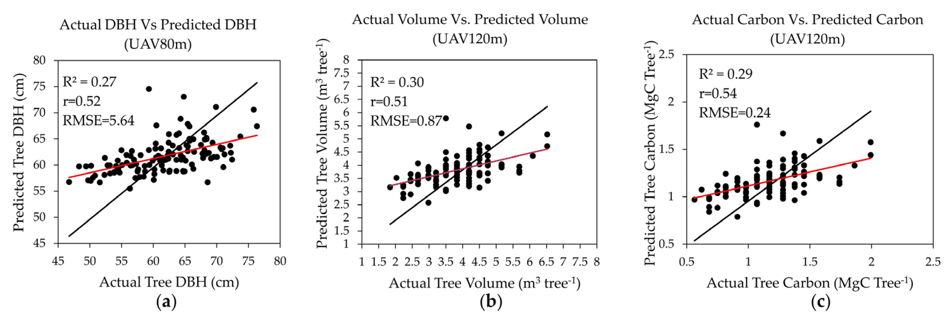
4.5. DBH, V, and CST
5. Discussion
5.1. Individual Tree Detection and Tree Density
5.2. Tree Height
5.3. Crown Delineation and CC Percentage
5.4. Tree DBH, V, and CST
5.5. Parameter Setting during the Photogrammetric Process
6. Conclusions
Author Contributions
Funding
Informed Consent Statement
Data Availability Statement
Acknowledgments
Conflicts of Interest
Appendix A

| Photogrammetric Process | Parameters |
|---|---|
| Image alignment | Accuracy: medium |
| Pair selection: Reference | |
| Key points: 40,000 | |
| Tie points: 1000 | |
| Guided marker positioning | 4 |
| Camera optimization parameters | F, b1, b2, cx, cy, k1–k4, p1, p2 |
| Building dense cloud | Quality: medium |
| Depth filtering: Mild | |
| Quality: medium | |
| Depth filtering: mild | |
| Building mesh | Surface type: medium |
| Source data: Dense cloud | |
| Interpolation: Disabled | |
| Face count: high | |
| Building DEM | Type: Geographic |
| Source data: Dense cloud | |
| Interpolation: enabled | |
| Building orthomosaic | Type: Geographic |
| Surface: DEM | |
| Blending mode: Mosaic | |
| Enable hole filling |
| Photogrammetric Process | Setting | UAV 80 m | UAV 120 m |
|---|---|---|---|
| Image alignment | Matching time | 15 min 34 s | 4 min 9 s |
| Alignment time | 25 min 55 s | 3 min 34 s | |
| Camera optimization | Optimization time | 1 min 13 s | 13 s |
| Building dense cloud | Processing time | 1 h 1 min | 18 min 5 s |
| Generation time | 2 h 7 min | 18 min 5 s | |
| Depth map and reconstruct | 1 h 30 min | 1 h 7 min | |
| Building DEM | Processing time | 2 min 6 s | 15 s |
| Building Orthomosaic | Processing time | 1 h 28 min | 1 h 5 min |
| Systems used | Software: Agsoft Metashape Professional Software version: 1.8.4 build 14856 OS: Windows 64 bit RAM: 31.71 GB CPU: 11th Gen Inter(R) Core (TM) i7-11800H @2.30 GHz GPU: NVIDIA GeForce RTX 3050 Ti Laptop GPU | ||
| UAV Attribute | UAV 80 m | UAV 120 m |
|---|---|---|
| Acquired images | 1257 | 372 |
| Flying altitude | 80 m | 120 m |
| Point density | 931 points/m2 | 328 points/m2 |
| Pixel resolution | 3.25 cm/pix | 5.39 cm/pix |
| Image resolution | 8192 × 5460 pix | 8192 × 5460 pix |
| Ground resolution | 0.813 cm/pix | 1.35 cm/pix |
| Tie points | 1,109,968 | 483,325 |
| Projections | 3,707,621 | 1,030,596 |
| Mean reprojection error (pixel) | 2.84 pix | 3.04 pix |
| Total error with GCPs | 0.331 pix | 0.367 pix |
| Dense clouds | 136,581,158 | 74,639,588 |
| Coordinate system | JGD2000 Japan–19 zone XII/GSIGEO 2000 geoid | |


References
- Yang, Z.; Zheng, Q.; Zhuo, M.; Zeng, H.; Hogan, J.A.; Lin, T.C. A Culture of Conservation: How an Ancient Forest Plantation Turned into an Old-Growth Forest Reserve–The Story of the Wamulin Forest. People Nat. 2021, 3, 1014–1024. [Google Scholar] [CrossRef]
- Hoshi, H. Forest Tree Genetic Resources Conservation Stands of Japanese Larch (Larix kaempferi (Lamb.) Carr.); Genetic Resources Department, Forest Tree Breeding Center: Ibaraki, Japan, 2004; Volume 1. Available online: https://www.ffpri.affrc.go.jp/ftbc/research/kakonokouhousi/documents/e-tokubetu.pdf (accessed on 1 March 2023).
- Sato, M.; Seki, K.; Kita, K.; Moriguchi, Y.; Hashimoto, M.; Yunoki, K.; Ohnishi, M. Comparative Analysis of Diterpene Composition in the Bark of the Hybrid Larch F1, Larix gmelinii var. japonica × L. kaempferi and their Parent Trees. J. Wood Sci. 2009, 55, 32–40. [Google Scholar] [CrossRef]
- Mishima, K.; Hirakawa, H.; Iki, T.; Fukuda, Y.; Hirao, T.; Tamura, A.; Takahashi, M. Comprehensive Collection of Genes and Comparative Analysis of Full-Length Transcriptome Sequences from Japanese Larch (Larix kaempferi) and Kuril Larch (Larix gmelinii var. japonica). BMC Plant Biol. 2022, 22, 470. [Google Scholar] [CrossRef] [PubMed]
- Nagamitsu, T.; Nagasaka, K.; Yoshimaru, H.; Tsumura, Y. Provenance Tests for Survival and Growth of 50-Year-Old Japanese Larch (Larix kaempferi) Trees related to Climatic Conditions in Central Japan. Tree Genet. Genomes 2014, 10, 87–99. [Google Scholar] [CrossRef]
- Nagaike, T. Snag Abundance and Species Composition in a Managed Forest Landscape in Central Japan Composed of Larix kaempferi Plantations and Secondary Broadleaf Forests. Silva Fenn. 2009, 43, 755–766. [Google Scholar] [CrossRef][Green Version]
- Takata, K.; Kurlnobu, S.; Koizumi, A.; Yasue, K.; Tamai, Y.; Kisanuki, M. Bibliography on Japanese Larch (Larix kaempferi (Lamb.) Carr.). Eurasian J. For. Res. 2005, 8, 111–126. [Google Scholar]
- Forestry Agency. State of Japan’s Forests and Forest Management-3rd Country Report of Japan to the Montreal Process; Japan, 2019. Available online: https://www.maff.go.jp/e/policies/forestry/attach/pdf/index-8.pdf (accessed on 20 March 2023).
- Kitao, N. Current State of Larch-Forestry in Hokkaido [Japan]: Area Studies for the Management of Experiment Forests of Kyoto University. Bull. Kyoto Univ. For. 1983, 55, 107–121. (In Japanese) [Google Scholar]
- Torita, H.; Masaka, K. Influence of Planting Density and Thinning on Timber Productivity and Resistance to Wind Damage in Japanese Larch (Larix kaempferi) Forests. J. Environ. Manag. 2020, 268, 110298. [Google Scholar] [CrossRef]
- Krause, S.; Sanders, T.G.M.; Mund, J.P.; Greve, K. UAV-Based Photogrammetric Tree Height Measurement for Intensive Forest Monitoring. Remote Sens. 2019, 11, 758. [Google Scholar] [CrossRef]
- Phalla, T.; Ota, T.; Mizoue, N.; Kajisa, T.; Yoshida, S.; Vuthy, M.; Heng, S. The Importance of Tree Height in Estimating Individual Tree Biomass while Considering Errors in Measurements and Allometric Models. Agrivita 2018, 40, 131–140. [Google Scholar] [CrossRef]
- Ramli, M.F.; Tahar, K.N. Homogeneous Tree Height Derivation from Tree Crown Delineation using Seeded Region Growing (SRG) Segmentation. Geo-Spat. Inf. Sci. 2020, 23, 195–208. [Google Scholar] [CrossRef]
- Panagiotidis, D.; Abdollahnejad, A.; Surový, P.; Chiteculo, V. Determining Tree Height and Crown Diameter from High-Resolution UAV Imagery. Int. J. Remote Sens. 2017, 38, 2392–2410. [Google Scholar] [CrossRef]
- Jayathunga, S.; Owari, T.; Tsuyuki, S.; Hirata, Y. Potential of UAV Photogrammetry for Characterization of Forest Canopy Structure in Uneven-Aged Mixed Conifer–Broadleaf Forests. Int. J. Remote Sens. 2020, 41, 53–73. [Google Scholar] [CrossRef]
- Sadeghi, S.M.M.; Attarod, P.; Pypker, T.G. Differences in Rainfall Interception during the Growing and Non-Growing Seasons in a Fraxinus rotundifolia Mill. Plantation Located in a Semiarid Climate. J. Agr. Sci. Tech. 2015, 17, 145–156. [Google Scholar]
- Thenkabail, P.S. Land Resources Monitoring, Modeling, and Mapping with Remote Sensing; Thenkabail, P.S., Ed.; CRC Press: Boca Raton, FL, USA, 2015; ISBN 9780429089442. [Google Scholar]
- Gao, H.; Bi, H.; Li, F. Modelling Conifer Crown Profiles as Nonlinear Conditional Quantiles: An Example with Planted Korean Pine in Northeast China. For. Ecol. Manag. 2017, 398, 101–115. [Google Scholar] [CrossRef]
- Valjarević, A.; Djekić, T.; Stevanović, V.; Ivanović, R.; Jandziković, B. GIS Numerical and Remote Sensing Analyses of Forest Changes in the Toplica Region for the Period of 1953–2013. Appl. Geogr. 2018, 92, 131–139. [Google Scholar] [CrossRef]
- Avery, T.E.; Burkhart, H. Forest Measurements, 5th ed.; McGraw Hill: Boston, MA, USA, 2002. [Google Scholar]
- Thiel, C.; Schmullius, C. Comparison of UAV Photograph-Based and Airborne LiDAR-Based Point Clouds over Forest from a Forestry Application Perspective. Int. J. Remote Sens. 2017, 38, 2411–2426. [Google Scholar] [CrossRef]
- Zarco-Tejada, P.J.; Diaz-Varela, R.; Angileri, V.; Loudjani, P. Tree Height Quantification using Very High Resolution Imagery Acquired from an Unmanned Aerial Vehicle (UAV) and Automatic 3D Photo-Reconstruction Methods. Eur. J. Agron. 2014, 55, 89–99. [Google Scholar] [CrossRef]
- Gu, J.; Grybas, H.; Congalton, R.G. Individual Tree Crown Delineation from UAS Imagery Based on Region Growing and Growth Space Considerations. Remote Sens. 2020, 12, 2363. [Google Scholar] [CrossRef]
- Bohlin, J.; Wallerman, J.; Fransson, J.E.S. Forest Variable Estimation using Photogrammetric Matching of Digital Aerial Images in Combination with a High-Resolution DEM. Scand. J. For. Res. 2012, 27, 692–699. [Google Scholar] [CrossRef]
- Järnstedt, J.; Pekkarinen, A.; Tuominen, S.; Ginzler, C.; Holopainen, M.; Viitala, R. Forest Variable Estimation using a High-Resolution Digital Surface Model. ISPRS J. Photogramm. Remote Sens. 2012, 74, 78–84. [Google Scholar] [CrossRef]
- White, J.C.; Wulder, M.A.; Vastaranta, M.; Coops, N.C.; Pitt, D.; Woods, M. The Utility of Image-Based Point Clouds for Forest Inventory: A Comparison with Airborne Laser Scanning. Forests 2013, 4, 518–536. [Google Scholar] [CrossRef]
- Wang, X.; Zhao, Q.; Han, F.; Zhang, J.; Jiang, P. Canopy Extraction and Height Estimation of Trees in a Shelter Forest Based on Fusion of an Airborne Multispectral Image and Photogrammetric Point Cloud. J. Sens. 2021, 2021, 5519629. [Google Scholar] [CrossRef]
- Moe, K.T.; Owari, T.; Furuya, N.; Hiroshima, T.; Morimoto, J. Application of UAV Photogrammetry with LiDAR Data to Facilitate the Estimation of Tree Locations and DBH Values for High-Value Timber Species in Northern Japanese Mixed-Wood Forests. Remote Sens. 2020, 12, 2865. [Google Scholar] [CrossRef]
- Hastaoglu, K.Ö.; Gogsu, S.; Gul, Y. Determining the Relationship between the Slope and Directional Distribution of the UAV Point Cloud and the Accuracy of Various IDW Interpolation. Int. J. Eng. Geosci. 2022, 7, 161–173. [Google Scholar] [CrossRef]
- Xu, Z.; Shen, X.; Cao, L.; Coops, N.C.; Goodbody, T.R.H.; Zhong, T.; Zhao, W.; Sun, Q.; Ba, S.; Zhang, Z.; et al. Tree Species Classification using UAS-Based Digital Aerial Photogrammetry Point Clouds and Multispectral Imageries in Subtropical Natural Forests. Int. J. Appl. Earth Obs. Geoinf. 2020, 92, 102173. [Google Scholar] [CrossRef]
- Kaartinen, H.; Hyyppä, J.; Yu, X.; Vastaranta, M.; Hyyppä, H.; Kukko, A.; Holopainen, M.; Heipke, C.; Hirschmugl, M.; Morsdorf, F.; et al. An International Comparison of Individual Tree Detection and Extraction using Airborne Laser Scanning. Remote Sens. 2012, 4, 950–974. [Google Scholar] [CrossRef]
- Vauhkonen, J.; Seppänen, A.; Packalén, P.; Tokola, T. Improving Species-Specific Plot Volume Estimates Based on Airborne Laser Scanning and Image Data using Alpha Shape Metrics and Balanced Field Data. Remote Sens. Environ. 2012, 124, 534–541. [Google Scholar] [CrossRef]
- Guerra-Hernández, J.; Cosenza, D.N.; Rodriguez, L.C.E.; Silva, M.; Tomé, M.; Díaz-Varela, R.A.; González-Ferreiro, E. Comparison of ALS- and UAV(SfM)-Derived High-Density Point Clouds for Individual Tree Detection in Eucalyptus Plantations. Int. J. Remote Sens. 2018, 39, 5211–5235. [Google Scholar] [CrossRef]
- Kukunda, C.B.; Duque-Lazo, J.; González-Ferreiro, E.; Thaden, H.; Kleinn, C. Ensemble Classification of Individual Pinus Crowns from Multispectral Satellite Imagery and Airborne LiDAR. Int. J. Appl. Earth Obs. Geoinf. 2018, 65, 12–23. [Google Scholar] [CrossRef]
- Takahashi, T.; Yamamoto, K.; Senda, Y.; Tsuzuku, M. Estimating Individual Tree Heights of Sugi (Cryptomeria japonica D. Don) Plantations in Mountainous Areas using Small-Footprint Airborne LiDAR. J. For. Res. 2005, 10, 135–142. [Google Scholar] [CrossRef]
- Machimura, T.; Fujimoto, A.; Hayashi, K.; Takagi, H.; Sugita, S. A Novel Tree Biomass Estimation Model Applying the Pipe Model Theory and Adaptable to UAV-Derived Canopy Height Models. Forests 2021, 12, 258. [Google Scholar] [CrossRef]
- Iizuka, K.; Yonehara, T.; Itoh, M.; Kosugi, Y. Estimating Tree Height and Diameter at Breast Height (DBH) from Digital Surface Models and Orthophotos obtained with an Unmanned Aerial System for a Japanese Cypress (Chamaecyparis obtusa) Forest. Remote Sens. 2018, 10, 13. [Google Scholar] [CrossRef]
- Ota, T.; Ogawa, M.; Mizoue, N.; Fukumoto, K.; Yoshida, S. Forest Structure Estimation from a UAV-Based Photogrammetric Point Cloud in Managed Temperate Coniferous Forests. Forests 2017, 8, 343. [Google Scholar] [CrossRef]
- Popescu, S.C.; Wynne, R.H. Seeing the Trees in the Forest. Photogramm. Eng. Remote Sens. 2004, 70, 589–604. [Google Scholar] [CrossRef]
- Abdullah, S.; Tahar, K.N.; Abdul Rashid, M.F.; Osoman, M.A. Estimating Tree Height Based on Tree Crown from UAV Imagery. Malays. J. Sustain. Environ. 2022, 9, 99. [Google Scholar] [CrossRef]
- Jeronimo, S.M.A.; Kane, V.R.; Churchill, D.J.; McGaughey, R.J.; Franklin, J.F. Applying LiDAR Individual Tree Detection to Management of Structurally Diverse Forest Landscapes. J. For. 2018, 116, 336–346. [Google Scholar] [CrossRef]
- Koontz, M.J.; Latimer, A.M.; Mortenson, L.A.; Fettig, C.J.; North, M.P. Cross-Scale Interaction of Host Tree Size and Climatic Water Deficit Governs Bark Beetle-Induced Tree Mortality. Nat. Commun. 2021, 12, 129. [Google Scholar] [CrossRef]
- Swayze, N.C.; Tinkham, W.T.; Vogeler, J.C.; Hudak, A.T. Influence of Flight Parameters on UAS-Based Monitoring of Tree Height, Diameter, and Density. Remote Sens. Environ. 2021, 263, 112540. [Google Scholar] [CrossRef]
- Nasiri, V.; Darvishsefat, A.A.; Arefi, H.; Pierrot-Deseilligny, M.; Namiranian, M.; Le Bris, A. Unmanned Aerial Vehicles (UAV)-Based Canopy Height Modeling under Leaf-on and Leaf-off Conditions for Determining Tree Height and Crown Diameter (Case Study: Hyrcanian Mixed Forest). Can. J. For. Res. 2021, 51, 962–971. [Google Scholar] [CrossRef]
- Arzt, M.; Deschamps, J.; Schmied, C.; Pietzsch, T.; Schmidt, D.; Tomancak, P.; Haase, R.; Jug, F. LABKIT: Labeling and Segmentation Toolkit for Big Image Data. Front. Comput. Sci. 2022, 4, 10. [Google Scholar] [CrossRef]
- Grznárová, A.; Mokroš, M.; Surový, P.; Slavík, M.; Pondelík, M.; Mergani, J. The Crown Diameter Estimation from Fixed Wing Type of UAV Imagery. Int. Arch. Photogramm. Remote Sens. Spatial Inf. Sci.-ISPRS Arch. 2019, 42, 337–341. [Google Scholar] [CrossRef]
- Silva, C.A.; Hudak, A.T.; Vierling, L.A.; Valbuena, R.; Cardil, A.; Mohan, M.; de Almeida, D.R.A.; Broadbent, E.N.; Almeyda Zambrano, A.M.; Wilkinson, B.; et al. TREETOP: A Shiny-based Application and R Package for Extracting Forest Information from LiDAR Data for Ecologists and Conservationists. Methods Ecol. Evol. 2022, 13, 1164–1176. [Google Scholar] [CrossRef]
- Young, D.J.N.; Koontz, M.J.; Weeks, J.M. Optimizing Aerial Imagery Collection and Processing Parameters for Drone-Based Individual Tree Mapping in Structurally Complex Conifer Forests. Methods Ecol. Evol. 2022, 13, 1447–1463. [Google Scholar] [CrossRef]
- Maras, E.E.; Nasery, N. Investigating the Length, Area and Volume Measurement Accuracy of UAV-Based Oblique Photogrammetry Models Produced with and without Ground Control Points. Int. J. Eng. Geosci. 2023, 8, 32–51. [Google Scholar] [CrossRef]
- Lerma, J.L.; Navarro, S.; Cabrelles, M.; Villaverde, V. Terrestrial Laser Scanning and Close Range Photogrammetry for 3D Archaeological Documentation: The Upper Palaeolithic Cave of Parpalló as a Case Study. J. Archaeol. Sci. 2010, 37, 499–507. [Google Scholar] [CrossRef]
- Yakar, M.; Ulvi, A.; Yiğit, A.Y.; Alptekin, A. Discontinuity Set Extraction from 3D Point Clouds Obtained by UAV Photogrammetry in a Rockfall Site. Surv. Rev. 2023, 55, 416–428. [Google Scholar] [CrossRef]
- Godfrey, I.; Avard, G.; Brenes, J.P.S.; Cruz, M.M.; Meghraoui, K. Using Sniffer4D and SnifferV Portable Gas Detectors for UAS Monitoring of Degassing at the Turrialba Volcano Costa Rica. Adv. UAV 2023, 3, 54–90. [Google Scholar]
- Gómez, C.; Wulder, M.A.; Montes, F.; Delgado, J.A. Modeling Forest Structural Parameters in the Mediterranean Pines of Central Spain using QuickBird-2 Imagery and Classification and Regression Tree Analysis (CART). Remote Sens. 2012, 4, 135–159. [Google Scholar] [CrossRef]
- Morin, D.; Planells, M.; Guyon, D.; Villard, L.; Mermoz, S.; Bouvet, A.; Thevenon, H.; Dejoux, J.-F.; Le Toan, T.; Dedieu, G. Estimation and Mapping of Forest Structure Parameters from Open Access Satellite Images: Development of a Generic Method with a Study Case on Coniferous Plantation. Remote Sens. 2019, 11, 1275. [Google Scholar] [CrossRef]
- Jayathunga, S.; Owari, T.; Tsuyuki, S. Evaluating the Performance of Photogrammetric Products using Fixed-Wing UAV Imagery over a Mixed Conifer–Broadleaf Forest: Comparison with Airborne Laser Scanning. Remote Sens. 2018, 10, 187. [Google Scholar] [CrossRef]
- Gao, S.; Zhang, Z.; Cao, L. Individual Tree Structural Parameter Extraction and Volume Table Creation Based on Near-Field LiDAR Data: A Case Study in a Subtropical Planted Forest. Sensors 2021, 21, 8162. [Google Scholar] [CrossRef] [PubMed]
- Belmonte, A.; Sankey, T.; Biederman, J.A.; Bradford, J.; Goetz, S.J.; Kolb, T.; Woolley, T. UAV-derived Estimates of Forest Structure to Inform Ponderosa Pine Forest Restoration. Remote Sens. Ecol. Conserv. 2020, 6, 181–197. [Google Scholar] [CrossRef]
- Kameyama, S.; Sugiura, K. Effects of Differences in Structure from Motion Software on Image Processing of Unmanned Aerial Vehicle Photography and Estimation of Crown Area and Tree Height in Forests. Remote Sens. 2021, 13, 626. [Google Scholar] [CrossRef]
- Hao, Y.; Widagdo, F.R.A.; Liu, X.; Quan, Y.; Liu, Z.; Dong, L.; Li, F. Estimation and Calibration of Stem Diameter Distribution using UAV Laser Scanning Data: A Case Study for Larch (Larix olgensis) Forests in Northeast China. Remote Sens. Environ. 2022, 268, 112769. [Google Scholar] [CrossRef]
- Liu, K.; Shen, X.; Cao, L.; Wang, G.; Cao, F. Estimating Forest Structural Attributes using UAV-LiDAR Data in Ginkgo Plantations. ISPRS J. Photogramm. Remote Sens. 2018, 146, 465–482. [Google Scholar] [CrossRef]
- Navarro, A.; Young, M.; Allan, B.; Carnell, P.; Macreadie, P.; Ierodiaconou, D. The Application of Unmanned Aerial Vehicles (UAVs) to estimate Above-Ground Biomass of Mangrove Ecosystems. Remote Sens. Environ. 2020, 242, 111747. [Google Scholar] [CrossRef]
- Silva, C.A.; Hudak, A.T.; Vierling, L.A.; Loudermilk, E.L.; O’Brien, J.J.; Hiers, J.K.; Jack, S.B.; Gonzalez-Benecke, C.; Lee, H.; Falkowski, M.J.; et al. Imputation of Individual Longleaf Pine (Pinus palustris Mill.) Tree Attributes from Field and LiDAR Data. Can. J. Remote Sens. 2016, 42, 554–573. [Google Scholar] [CrossRef]
- Korpela, I.; Anttila, P.; Pitkänen, J. The Performance of a Local Maxima Method for Detecting Individual Tree Tops in Aerial Photographs. Int. J. Remote Sens. 2006, 27, 1159–1175. [Google Scholar] [CrossRef]
- Lindberg, E.; Hollaus, M. Comparison of Methods for Estimation of Stem Volume, Stem Number and Basal Area from Airborne Laser Scanning Data in a Hemi-Boreal Forest. Remote Sens. 2012, 4, 1004–1023. [Google Scholar] [CrossRef]
- Gao, T.; Gao, Z.; Sun, B.; Qin, P.; Li, Y.; Yan, Z. An Integrated Method for estimating Forest-Canopy Closure Based on UAV LiDAR Data. Remote Sens. 2022, 14, 4317. [Google Scholar] [CrossRef]
- Cao, Y.; Ball, J.G.C.; Coomes, D.A.; Steinmeier, L.; Knapp, N.; Wilkes, P.; Disney, M.; Calders, K.; Burt, A.; Lin, Y.; et al. Benchmarking Airborne Laser Scanning Tree Segmentation Algorithms in Broadleaf Forests Shows High Accuracy Only for Canopy Trees. Int. J. Appl. Earth Obs. Geoinf. 2023, 123, 103490. [Google Scholar] [CrossRef]
- Mohan, M.; Leite, R.V.; Broadbent, E.N.; Wan Mohd Jaafar, W.S.; Srinivasan, S.; Bajaj, S.; Dalla Corte, A.P.; Do Amaral, C.H.; Gopan, G.; Saad, S.N.M.; et al. Individual Tree Detection using UAV-LiDAR and UAV-SfM Data: A Tutorial for Beginners. Open Geosci. 2021, 13, 1028–1039. [Google Scholar] [CrossRef]
- Fu, L.; Duan, G.; Ye, Q.; Meng, X.; Luo, P.; Sharma, R.P.; Sun, H.; Wang, G.; Liu, Q. Prediction of Individual Tree Diameter using a Nonlinear Mixed-Effects Modeling Approach and Airborne LiDAR Data. Remote Sens. 2020, 12, 1066. [Google Scholar] [CrossRef]
- Leite, R.; Silva, C.; Mohan, M.; Cardil, A.; Almeida, D.; Carvalho, S.; Jaafar, W.; Guerra-Hernández, J.; Weiskittel, A.; Hudak, A.; et al. Individual Tree Attribute Estimation and Uniformity Assessment in Fast-Growing Eucalyptus spp. Forest Plantations using LiDAR and Linear Mixed-Effects Models. Remote Sens. 2020, 12, 3599. [Google Scholar] [CrossRef]
- Liang, X.; Wang, Y.; Jaakkola, A.; Kukko, A.; Kaartinen, H.; Hyyppa, J.; Honkavaara, E.; Liu, J. Forest Data Collection using Terrestrial Image-Based Point Clouds from a Handheld Camera Compared to Terrestrial and Personal Laser Scanning. IEEE Trans. Geosci. Remote Sens. 2015, 53, 5117–5132. [Google Scholar] [CrossRef]
- Piermattei, L.; Karel, W.; Wang, D.; Wieser, M.; Mokroš, M.; Surový, P.; Koreň, M.; Tomaštík, J.; Pfeifer, N.; Hollaus, M. Terrestrial Structure from Motion Photogrammetry for Deriving Forest Inventory Data. Remote Sens. 2019, 11, 950. [Google Scholar] [CrossRef]
- Sun, Y.; Jin, X.; Pukkala, T.; Li, F. Predicting Individual Tree Diameter of Larch (Larix olgensis) from UAV-LiDAR Data using Six Different Algorithms. Remote Sens. 2022, 14, 1125. [Google Scholar] [CrossRef]
- Hirschmugl, M.; Sobe, C.; Di Filippo, A.; Berger, V.; Kirchmeir, H.; Vandekerkhove, K. Review on the Possibilities of Mapping Old-Growth Temperate Forests by Remote Sensing in Europe. Environ. Model. Assess. 2023, 28, 761–785. [Google Scholar] [CrossRef]
- Qiu, Z.; Feng, Z.-K.; Wang, M.; Li, Z.; Lu, C. Application of UAV Photogrammetric System for Monitoring Ancient Tree Communities in Beijing. Forests 2018, 9, 735. [Google Scholar] [CrossRef]
- Holiaka, D.; Kato, H.; Yoschenko, V.; Onda, Y.; Igarashi, Y.; Nanba, K.; Diachuk, P.; Holiaka, M.; Zadorozhniuk, R.; Kashparov, V.; et al. Scots Pine Stands Biomass Assessment using 3D Data from Unmanned Aerial Vehicle Imagery in the Chernobyl Exclusion Zone. J. Environ. Manag. 2021, 295, 113319. [Google Scholar] [CrossRef] [PubMed]
- Zhou, X.; Zhang, X. Individual Tree Parameters Estimation for Plantation Forests Based on UAV Oblique Photography. IEEE Access 2020, 8, 96184–96198. [Google Scholar] [CrossRef]
- Moe, K.T.; Owari, T.; Furuya, N.; Hiroshima, T. Comparing Individual Tree Height Information Derived from Field Surveys, LiDAR and UAV-DAP for High-Value Timber Species in Northern Japan. Forests 2020, 11, 223. [Google Scholar] [CrossRef]
- Greenhouse Gas Inventory Office of Japan and Ministry of Environment, Japan (Ed.) National Greenhouse Gas Inventory Report of JAPAN 2023; Center for Global Environmental Research, Earth System Division, National Institute for Environmental Studies: Japan. Available online: https://www.nies.go.jp/gio/archive/nir/jqjm1000001v3c7t-att/NIR-JPN-2023-v3.0_gioweb.pdf (accessed on 3 February 2023).
- Tavasci, L.; Lambertini, A.; Donati, D.; Girelli, V.A.; Lattanzi, G.; Castellaro, S.; Gandolfi, S.; Borgatti, L. A Laboratory for the Integration of Geomatic and Geomechanical Data: The Rock Pinnacle “Campanile Di Val Montanaia”. Remote Sens. 2023, 15, 4854. [Google Scholar] [CrossRef]
- Mot, L.; Hong, S.; Charoenjit, K.; Zhang, H. Tree Height Estimation using Field Measurement and Low-Cost Unmanned Aerial Vehicle (UAV) at Phnom Kulen National Park of Cambodia. In Proceedings of the 2021 9th International Conference on Agro-Geoinformatics, Agro-Geoinformatics 2021, Shenzhen, China, 26–29 July 2021. [Google Scholar]
- Pourreza, M.; Moradi, F.; Khosravi, M.; Deljouei, A.; Vanderhoof, M.K. GCPs-Free Photogrammetry for estimating Tree Height and Crown Diameter in Arizona Cypress Plantation using UAV-Mounted GNSS RTK. Forests 2022, 13, 1905. [Google Scholar] [CrossRef]
- Mohan, M.; Silva, C.A.; Klauberg, C.; Jat, P.; Catts, G.; Cardil, A.; Hudak, A.T.; Dia, M. Individual Tree Detection from Unmanned Aerial Vehicle (UAV) Derived Canopy Height Model in an Open Canopy Mixed Conifer Forest. Forests 2017, 8, 340. [Google Scholar] [CrossRef]
- Ahongshangbam, J.; Röll, A.; Ellsäßer, F.; Hendrayanto; Hölscher, D. Airborne Tree Crown Detection for Predicting Spatial Heterogeneity of Canopy Transpiration in a Tropical Rainforest. Remote Sens. 2020, 12, 651. [Google Scholar] [CrossRef]
- Goutte, C.; Gaussier, E. A Probabilistic Interpretation of Precision, Recall and F-Score, with Implication for Evaluation. In Proceedings of the Lecture Notes in Computer Science; Springer: Berlin/Heidelberg, Germany, 2005; Volume 3408, pp. 345–359. [Google Scholar]
- Sokolova, M.; Japkowicz, N.; Szpakowicz, S. Beyond Accuracy, F-Score and ROC: A Family of Discriminant Measures for Performance Evaluation. In AI 2006: Advances in Artificial Intelligence; AI 2006. Lecture Notes in Computer Science; Sattar, A., Kang, B., Eds.; Springer: Berlin/Heidelberg, Germany, 2006; Volume 4304, pp. 1015–1021. [Google Scholar] [CrossRef]
- Akaike, H. Information Theory and an Extension of the Maximum Likelihood Principle; Selected Papers of Hirotugu Akaike. Springer Series in Statistics; Parzen, E., Tanabe, K., Kitagawa, G., Eds.; Springer: New York, NY, USA, 1998; pp. 199–213. [Google Scholar] [CrossRef]
- Kock, N.; Lynn, G.S. Lateral Collinearity and Misleading Results in Variance-Based SEM: An Illustration and Recommendations. J. Assoc. Inf. Syst. 2012, 13, 546–580. [Google Scholar] [CrossRef]
- Xiao, C.; Qin, R.; Huang, X.; Li, J. A Study of using Fully Convolutional Network for Treetop Detection on Remote Sensing Data. In Proceedings of the ISPRS Annals of the Photogrammetry, Remote Sensing and Spatial Information Sciences, Karlsruhe, Germany; 2018; Volume 4, pp. 163–169. Available online: https://isprs-annals.copernicus.org/articles/IV-1/163/2018/isprs-annals-IV-1-163-2018.pdf (accessed on 20 April 2023).
- Nevalainen, O.; Honkavaara, E.; Tuominen, S.; Viljanen, N.; Hakala, T.; Yu, X.; Hyyppä, J.; Saari, H.; Pölönen, I.; Imai, N.N.; et al. Individual Tree Detection and Classification with UAV-Based Photogrammetric Point Clouds and Hyperspectral Imaging. Remote Sens. 2017, 9, 185. [Google Scholar] [CrossRef]
- Islami, M.M.; Rusolono, T.; Setiawan, Y.; Rahadian, A.; Hudjimartsu, S.A.; Prasetyo, L.B. Height, Diameter and Tree Canopy Cover Estimation Based on Unmanned Aerial Vehicle (UAV) Imagery with Various Acquisition Height. Media Konserv. 2021, 26, 17–27. [Google Scholar] [CrossRef]
- White, J. Estimating the Age of Large & Veteran Trees in Britain; Forestry Commission: Edinburgh, Scotland, 1998; Available online: https://www.ancienttreeforum.org.uk/wp-content/uploads/2015/03/John-White-estimating-file-pdf.pdf (accessed on 28 April 2023).
- Gilmartin, E. Ancient and Veteran Trees: An Assessment Guid; The Woodland Trust: Grantham, UK, 2022.
- Cai, S.; Zhang, W.; Liang, X.; Wan, P.; Qi, J.; Yu, S.; Yan, G.; Shao, J. Filtering Airborne LiDAR Data Through Complementary Cloth Simulation and Progressive TIN Densification Filters. Remote Sens. 2019, 11, 1037. [Google Scholar] [CrossRef]
- Tang, S.; Dong, P.; Buckles, B.P. Three-Dimensional Surface Reconstruction of Tree Canopy from Lidar Point Clouds using a Region-Based Level Set Method. Int. J. Remote Sens. 2013, 34, 1373–1385. [Google Scholar] [CrossRef]
- Yoshida, T.; Hasegawa, M.; Taira, H.; Noguchi, M. Stand Structure and Composition of a 60-Year-Old Larch (Larix kaempferi) Plantation with Retained Hardwoods. J. For. Res. 2005, 10, 351–358. [Google Scholar] [CrossRef]
- Kita, K.; Fujimoto, T.; Uchiyama, K.; Kuromaru, M.; Akutsu, H. Estimated Amount of Carbon Accumulation of Hybrid Larch in Three 31-Year-Old Progeny Test Plantations. J. Wood Sci. 2009, 55, 425–434. [Google Scholar] [CrossRef]
- Yu, X.; Hyyppä, J.; Vastaranta, M.; Holopainen, M.; Viitala, R. Predicting Individual Tree Attributes from Airborne Laser Point Clouds Based on the Random Forests Technique. ISPRS J. Photogramm. Remote Sens. 2011, 66, 28–37. [Google Scholar] [CrossRef]
- Chen, Q.; Gong, P.; Baldocchi, D.; Tian, Y.Q. Estimating Basal Area and Stem Volume for Individual Trees from Lidar Data. Photogramm. Eng. Remote Sens. 2007, 73, 1355–1365. [Google Scholar] [CrossRef]
- Jucker, T.; Caspersen, J.; Chave, J.; Antin, C.; Barbier, N.; Bongers, F.; Dalponte, M.; van Ewijk, K.Y.; Forrester, D.I.; Haeni, M.; et al. Allometric Equations for Integrating Remote Sensing Imagery into Forest Monitoring Programmes. Glob. Chang. Biol. 2017, 23, 177–190. [Google Scholar] [CrossRef]
- Hulshof, C.M.; Swenson, N.G.; Weiser, M.D. Tree Height-Diameter Allometry across the United States. Ecol. Evol. 2015, 5, 1193–1204. [Google Scholar] [CrossRef]
- Mousavi, V.; Varshosaz, M.; Remondino, F. Evaluating Tie Points Distribution, Multiplicity and Number on the Accuracy of UAV Photogrammetry Blocks. Int. Arch. Photogramm. Remote Sens. Spat. Inf. Sci. 2021, XLIII, 39–46. [Google Scholar] [CrossRef]
- Snavely, N.; Seitz, S.M.; Szeliski, R. Modeling the World from Internet Photo Collections. Int. J. Comput. Vis. 2008, 80, 189–210. [Google Scholar] [CrossRef]
- Lowe, D.G. Distinctive Image Features from Scale-Invariant Keypoints. Int. J. Comput. Vis. 2004, 60, 91–110. [Google Scholar] [CrossRef]
- Barazzetti, L. Network Design in Close-Range Photogrammetry with Short Baseline Images. ISPRS Ann. Photogramm. Remote Sens. Spat. Inf. Sci. 2017, IV–2, 17–23. [Google Scholar] [CrossRef]
- Farella, E.M.; Torresani, A.; Remondino, F. Refining the Joint 3D Processing of Terrestrial and UAV Images using Quality Measures. Remote Sens. 2020, 12, 2873. [Google Scholar] [CrossRef]
- Mousavi, V.; Varshosaz, M.; Rashidi, M.; Li, W. A New Multi-Criteria Tie Point Filtering Approach to increase the Accuracy of UAV Photogrammetry Models. Drones 2022, 6, 413. [Google Scholar] [CrossRef]
- Izere, P. Plant Height Estimation Using RTK-GNSS Enabled Unmanned Aerial Vehicle (UAV) Photogrammetry. Master’s Thesis, University of Nebraska, Lincoln, NE, USA, 2023. [Google Scholar]
- Tomaštík, J.; Mokroš, M.; Surový, P.; Grznárová, A.; Merganič, J. UAV RTK/PPK Method—An Optimal Solution for Mapping Inaccessible Forested Areas? Remote Sens. 2019, 11, 721. [Google Scholar] [CrossRef]
- Zhao, B.; Li, J.; Wang, L.; Shi, Y. Positioning Accuracy Assessment of a Commercial RTK UAS. In Proceedings of the Autonomous Air and Ground Sensing Systems for Agricultural Optimization and Phenotyping V; SPIE Defense + Commercial Sensing: 2020, 1141409; p. 8. Available online: https://www.spiedigitallibrary.org/conference-proceedings-of-spie/11414/2557899/Positioning-accuracy-assessment-of-a-commercial-RTK-UAS/10.1117/12.2557899.short?SSO=1 (accessed on 20 September 2023).
- Štroner, M.; Urban, R.; Seidl, J.; Reindl, T.; Brouček, J. Photogrammetry using UAV-Mounted GNSS RTK: Georeferencing Strategies without GCPs. Remote Sens. 2021, 13, 1336. [Google Scholar] [CrossRef]
- Tahar, K.N. An Evaluation on Different Number of Ground Control Points in Unmanned Aerial Vehicle Photogrammetric Block. Int. Arch. Photogramm. Remote Sens. Spat. Inf. Sci. 2013, XL–2, 27–29. [Google Scholar] [CrossRef]
- Kalacska, M.; Lucanus, O.; Arroyo-Mora, J.; Laliberté, É.; Elmer, K.; Leblanc, G.; Groves, A. Accuracy of 3D Landscape Reconstruction without Ground Control Points using Different UAS Platforms. Drones 2020, 4, 13. [Google Scholar] [CrossRef]
- Stott, E.; Williams, R.D.; Hoey, T.B. Ground Control Point Distribution for Accurate Kilometre-Scale Topographic Mapping using an RTK-GNSS Unmanned Aerial Vehicle and SfM Photogrammetry. Drones 2020, 4, 55. [Google Scholar] [CrossRef]
- Štroner, M.; Urban, R.; Reindl, T.; Seidl, J.; Brouček, J. Evaluation of the Georeferencing Accuracy of a Photogrammetric Model using a Quadrocopter with Onboard GNSS RTK. Sensors 2020, 20, 2318. [Google Scholar] [CrossRef]
- Martínez-Carricondo, P.; Agüera-Vega, F.; Carvajal-Ramírez, F.; Mesas-Carrascosa, F.-J.; García-Ferrer, A.; Pérez-Porras, F.-J. Assessment of UAV-Photogrammetric Mapping Accuracy Based on Variation of Ground Control Points. Int. J. Appl. Earth Obs. Geoinf. 2018, 72, 1–10. [Google Scholar] [CrossRef]
- Yu, J.J.; Kim, D.W.; Lee, E.J.; Son, S.W. Determining the Optimal Number of Ground Control Points for Varying Study Sites through Accuracy Evaluation of Unmanned Aerial System-Based 3D Point Clouds and Digital Surface Models. Drones 2020, 4, 49. [Google Scholar] [CrossRef]
- Frey, J.; Kovach, K.; Stemmler, S.; Koch, B. UAV Photogrammetry of Forests as a Vulnerable Process. A Sensitivity Analysis for a Structure from Motion RGB-Image Pipeline. Remote Sens. 2018, 10, 912. [Google Scholar] [CrossRef]

 ,
,  ,
,  ,
,  represents the save (tap to save current settings and create a mission flight), delete selected waypoint (tap to delete the selected waypoint), start flight button (tap to perform the flight mission), and clear waypoints (tap to clear all the added waypoint), respectively. The meaning of location 1. 東京大学樹木園桜公園 and 2. 樹木園 are the cherry blossom park of the University of Tokyo arboretum and arboretum, respectively.
, , , represents the save (tap to save current settings and create a mission flight), delete selected waypoint (tap to delete the selected waypoint), start flight button (tap to perform the flight mission), and clear waypoints (tap to clear all the added waypoint), respectively. The meaning of location 1. 東京大学樹木園桜公園 and 2. 樹木園 are the cherry blossom park of the University of Tokyo arboretum and arboretum, respectively.
represents the save (tap to save current settings and create a mission flight), delete selected waypoint (tap to delete the selected waypoint), start flight button (tap to perform the flight mission), and clear waypoints (tap to clear all the added waypoint), respectively. The meaning of location 1. 東京大学樹木園桜公園 and 2. 樹木園 are the cherry blossom park of the University of Tokyo arboretum and arboretum, respectively.
, , , represents the save (tap to save current settings and create a mission flight), delete selected waypoint (tap to delete the selected waypoint), start flight button (tap to perform the flight mission), and clear waypoints (tap to clear all the added waypoint), respectively. The meaning of location 1. 東京大学樹木園桜公園 and 2. 樹木園 are the cherry blossom park of the University of Tokyo arboretum and arboretum, respectively.


| Field Parameter | Unit | Mean | SD * | Range |
|---|---|---|---|---|
| Tree height (TH) | m tree−1 | 35.20 | 3.27 | 25.80–42.90 |
| Tree diameter (DBH) | cm tree−1 | 60.94 | 7.14 | 45.45–79.93 |
| Basal area (BA) | m2 tree−1 | 0.30 | 0.07 | 0.16–0.50 |
| Stem volume (V) | m3 tree−1 | 3.76 | 1.10 | 1.84–7.42 |
| Carbon stock (CST) | MgC tree−1 | 1.15 | 0.34 | 0.56–2.27 |
| Tree density | stems ha–1 | 147 |
| UAV Parameter | Setting |
|---|---|
| Model | DJI Matrice 300 RTK (Da-Jiang Innovations, Shenzhen, China) |
| Camera model | DJI Zenmuse P1 RGB (Da-Jiang Innovations, Shenzhen, China) |
| Lens specifications * | Sensor Dimensions: 35.000 mm × 23.328 mm Resolution: 8192 × 5460 Focal Length: 35 mm Pixel Size: 4.39 × 4.39 μm |
| Flight altitude | 80 m and 120 m |
| Front overlap | 90% |
| Side overlap | 90% |
| Flight time | 30 min |
| Flight take-off speed | 15 m/s |
| Average Flight speed—80 m | 5 m/s |
| Average Flight speed—120 m | 7 m/s |
| Ground Sampling Distance—80 m | 1.00 cm/pixel |
| Ground Sampling Distance—120 m | 1.51 cm/pixel |
| UAV Altitude | Filtering Method * | Search Radius/Sigma (m) | Window Size (m)/Search Method | UAV Treetop ** |
|---|---|---|---|---|
| UAV 80 m | LML | 1 | circle | 304 |
| 2 | circle | 182 | ||
| 3 | circle | 135 | ||
| LMG | 1 | circle | 316 | |
| 2 | circle | 224 | ||
| 3 | circle | 184 | ||
| 4 | circle | 182 | ||
| 5 | circle | 182 | ||
| SM | FWS: 3 × 3, SWS: 3 × 3 | 242 | ||
| FWS: 5 × 5, SWS: 3 × 3 | 151 | |||
| SG | 1 | FWS: 3 × 3 | 258 | |
| 2 | FWS: 3 × 3 | 245 | ||
| 3 | FWS: 3 × 3 | 244 | ||
| 1 | FWS: 5 × 5 | 154 | ||
| 2 | FWS: 5 × 5 | 152 | ||
| 3 | FWS: 5 × 5 | 153 | ||
| UAV 120 m | LML | 1 | circle | 300 |
| 2 | circle | 182 | ||
| 3 | circle | 131 | ||
| LMG | 1 | circle | 317 | |
| 2 | circle | 226 | ||
| 3 | circle | 190 | ||
| 4 | circle | 187 | ||
| 5 | circle | 187 | ||
| SM | FWS: 3 × 3, SWS: 3 × 3 | 243 | ||
| FWS: 5 × 5, SWS: 3 × 3 | 149 | |||
| SG | 1 | FWS: 3 × 3 | 249 | |
| 2 | FWS: 3 × 3 | 244 | ||
| 1 | FWS: 5 × 5 | 150 | ||
| 2 | FWS: 5 × 5 | 149 |
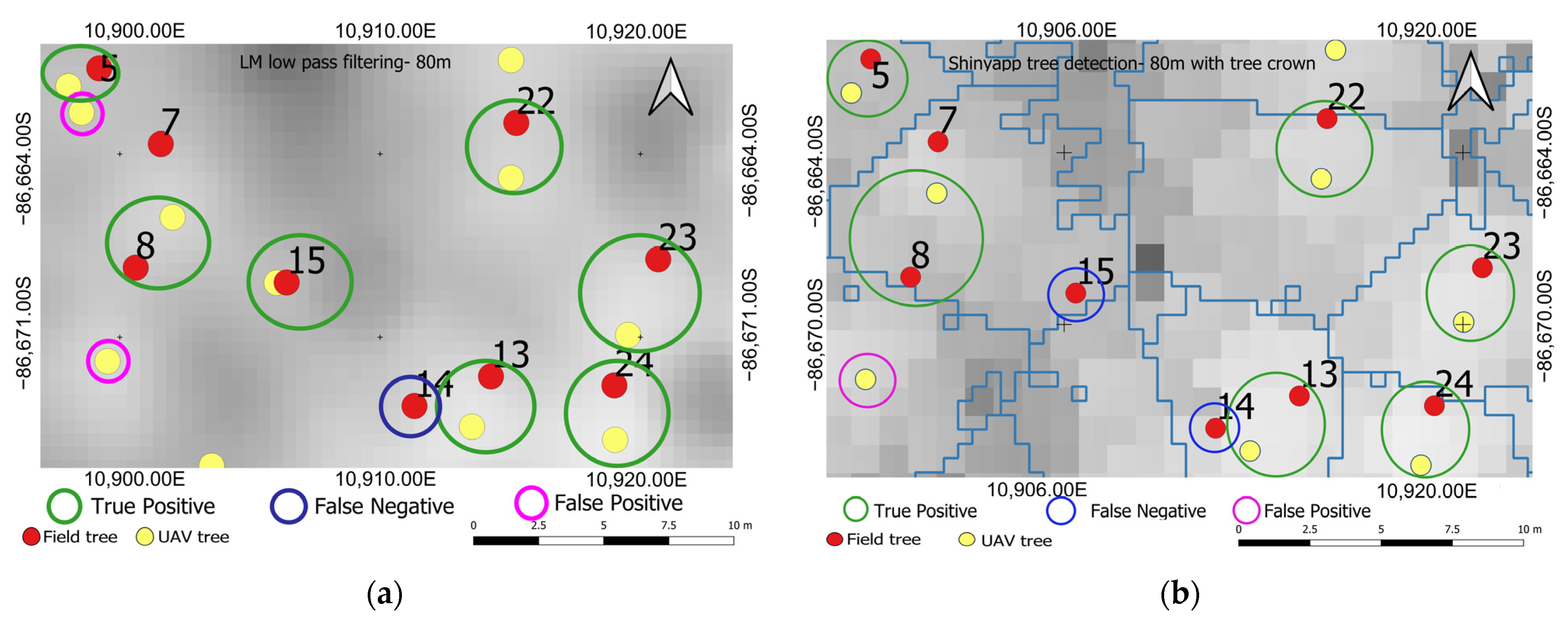
| UAV Altitude | Filtering Method * | UAV Treetop | Tree Density | TP | FP | FN | Precision | Recall | F-Score |
|---|---|---|---|---|---|---|---|---|---|
| UAV 80 m | LML2 | 176 | 189.09 | 124 | 52 | 12 | 0.91 | 0.70 | 0.79 |
| SM5 | 144 | 154.71 | 122 | 22 | 14 | 0.90 | 0.85 | 0.87 | |
| SG2 | 145 | 155.78 | 122 | 23 | 14 | 0.90 | 0.84 | 0.87 | |
| UAV 120 m | LML2 | 178 | 191.24 | 119 | 59 | 17 | 0.88 | 0.67 | 0.76 |
| SM5 | 142 | 152.56 | 116 | 26 | 20 | 0.85 | 0.82 | 0.83 | |
| SG2 | 142 | 152.56 | 115 | 27 | 21 | 0.85 | 0.81 | 0.83 |
| Field and UAV Altitude | Filtering Method * | Mean TH ± SD (m) | Maximum | Minimum |
|---|---|---|---|---|
| Field | Field TH (n = 136) | 35.23 ± 3.27 | 42.90 | 25.80 |
| UAV 80 m | LML2 (n = 136) | 35.49 ± 2.81 | 40.62 | 26.71 |
| SM5 (n = 123) | 35.63 ± 2.55 | 40.62 | 27.40 | |
| SG2 (n = 122) | 35.65 ± 2.52 | 40.62 | 27.40 | |
| UAV 120 m | LML2 (n = 125) | 35.76 ± 2.89 | 41.97 | 27.18 |
| SM5 (n = 123) | 35.08 ± 2.63 | 40.85 | 27.37 | |
| SG2 (n = 122) | 35.81 ± 2.62 | 40.86 | 27.15 |
| UAV Altitude | Filtering Method * | Mean TH ± SD (m) | Maximum | Minimum | CC Larch (%) | CC All (%) |
|---|---|---|---|---|---|---|
| UAV 80 m | Manual CA (n = 136) | 56.65 ± 21.27 | 144.76 | 23.89 | 74.74 | 77.44 |
| SM5 (n = 98) | 63.72 ± 18.73 | 106.00 | 31.25 | 92.02 | 96.05 | |
| SG2 (n = 98) | 63.83 ± 18.65 | 106.00 | 31.25 | 92.77 | 96.06 | |
| UAV 120 m | Manual CA (n = 136) | 56.44 ± 21.24 | 144.76 | 23.89 | 74.74 | 77.44 |
| SM5 (n = 106) | 55.57 ± 14.33 | 100.50 | 19.50 | 78.72 | 82.29 | |
| SG2 (n = 95) | 56.64 ± 14.29 | 100.50 | 19.50 | 78.72 | 82.29 |
| UAV Altitude | Dependent Variable (Unit) | Independent Variables ** | Selected Model | Parameter Estimates | R2 | RMSE |
|---|---|---|---|---|---|---|
| UAV 80 m | DBH (cm) | SG_TH, ND, M_CA, C_peri | Intercept | 45.02948 *** | 0.27 | 5.64 |
| SG_TH | 0.20821 * | |||||
| M_CA | 0.16068 *** | |||||
| UAV 120 m | V (m3 tree−1) | SG_TH, M_CA, ND, SG_CA | Intercept | −0.773327 *** | 0.30 | 0.87 |
| SG_TH | 0.086222 * | |||||
| M_CA | 0.025442 *** | |||||
| C (MgC tree−1) | SG_TH, M_CA, ND, SG_CA | Intercept | −0.229230 *** | 0.29 | 0.24 | |
| SG_TH | 0.026223 * | |||||
| M_CA | 0.007716 *** |
Disclaimer/Publisher’s Note: The statements, opinions and data contained in all publications are solely those of the individual author(s) and contributor(s) and not of MDPI and/or the editor(s). MDPI and/or the editor(s) disclaim responsibility for any injury to people or property resulting from any ideas, methods, instructions or products referred to in the content. |
© 2023 by the authors. Licensee MDPI, Basel, Switzerland. This article is an open access article distributed under the terms and conditions of the Creative Commons Attribution (CC BY) license (https://creativecommons.org/licenses/by/4.0/).
Share and Cite
Karthigesu, J.; Owari, T.; Tsuyuki, S.; Hiroshima, T. UAV Photogrammetry for Estimating Stand Parameters of an Old Japanese Larch Plantation Using Different Filtering Methods at Two Flight Altitudes. Sensors 2023, 23, 9907. https://doi.org/10.3390/s23249907
Karthigesu J, Owari T, Tsuyuki S, Hiroshima T. UAV Photogrammetry for Estimating Stand Parameters of an Old Japanese Larch Plantation Using Different Filtering Methods at Two Flight Altitudes. Sensors. 2023; 23(24):9907. https://doi.org/10.3390/s23249907
Chicago/Turabian StyleKarthigesu, Jeyavanan, Toshiaki Owari, Satoshi Tsuyuki, and Takuya Hiroshima. 2023. "UAV Photogrammetry for Estimating Stand Parameters of an Old Japanese Larch Plantation Using Different Filtering Methods at Two Flight Altitudes" Sensors 23, no. 24: 9907. https://doi.org/10.3390/s23249907
APA StyleKarthigesu, J., Owari, T., Tsuyuki, S., & Hiroshima, T. (2023). UAV Photogrammetry for Estimating Stand Parameters of an Old Japanese Larch Plantation Using Different Filtering Methods at Two Flight Altitudes. Sensors, 23(24), 9907. https://doi.org/10.3390/s23249907