


Enhancing QoS of Telecom Networks through Server Load Management in Software-Defined Networking (SDN)


Abstract
:1. Introduction
Motivations and Significance of Research Technique
- (a)
- By applying the DASLM approach, there is less end-to-end latency delay, maximum throughput, and less queuing delays by avoiding elephant flows, equal load management, and efficient use of bandwidth can be achieved.
- (b)
- Bandwidth enhancement is obtained using the proposed (DASLM) technique.
- (c)
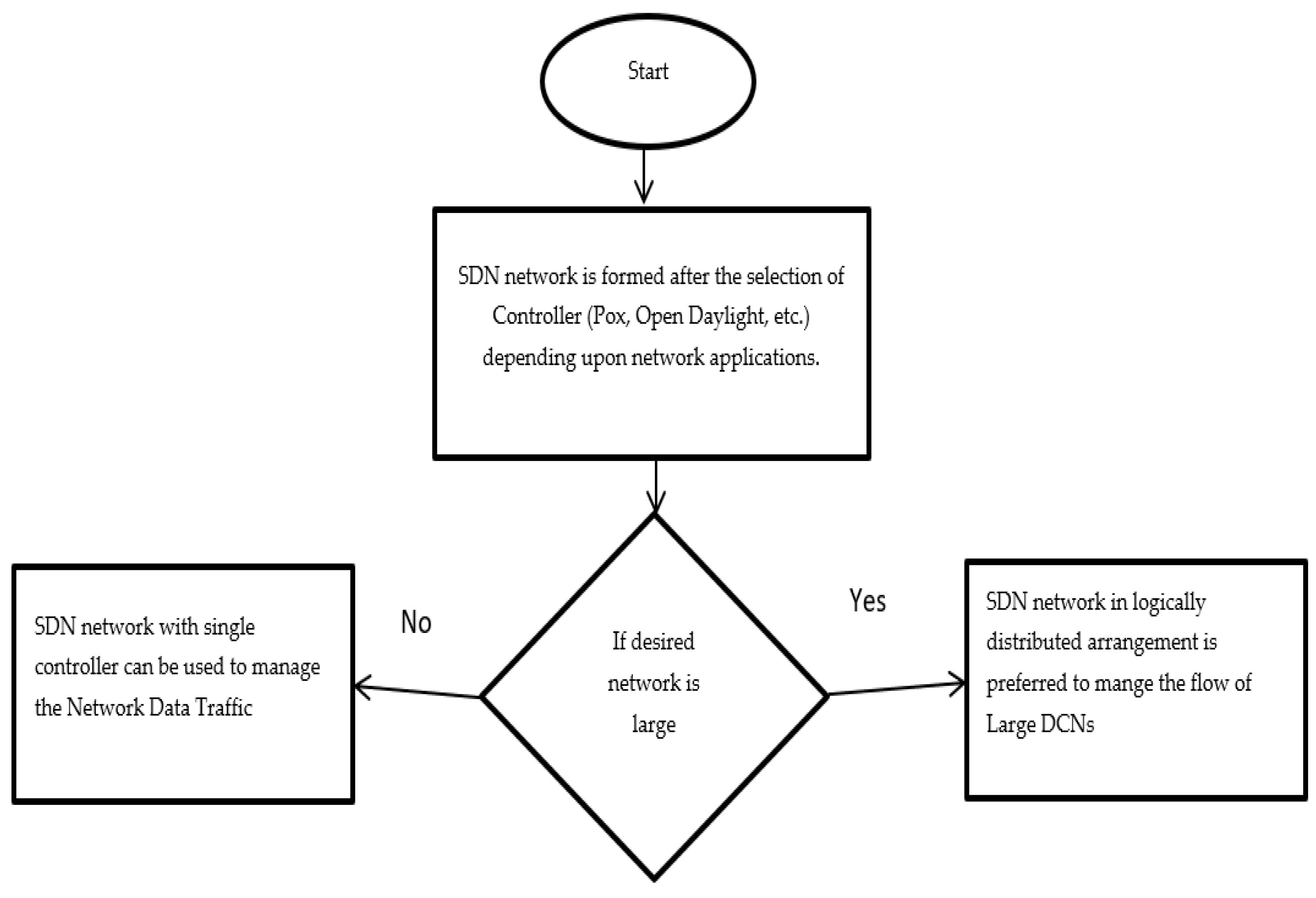
- In the case of large networks (more switches, hosts, data center servers), the single controller could become loaded, exhausted, and lead to a single-point failure. The solution mentioned in different research techniques, as discussed in Section 2.1, was to use multiple controllers (in the master-salve version). The major issues in the implementation of these methods involve the following:
- (1)
- The compatibility of two controllers.
- (2)
- Providing the data center server access to both controllers.
- (3)
- Switches flow managed by both controllers.
- (d)
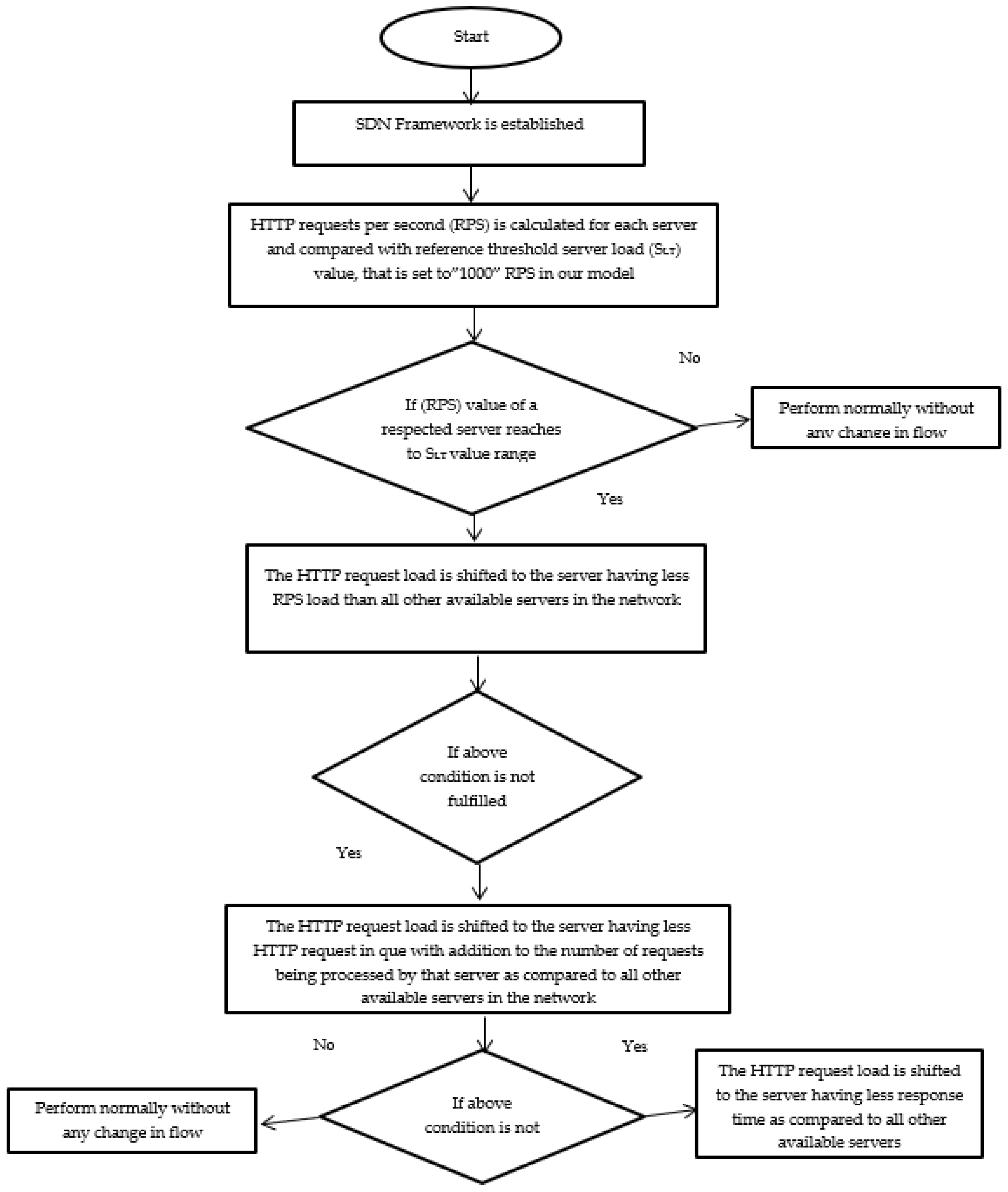
- The other major problem addressed in the proposed technique is the load balancing in the HTTP service provider servers by calculating the number of HTTP requests on each server and computing the server load. The HTTP request per second value (RPS) of each server is compared with the reference server load threshold (SLT) value (as explained in Section 3.1), which is set to a level of 1000 (HTTP requests per second) in our case. If the number of HTTP requests on the particular server has reached the (SLT) value, then that server is considered loaded and is removed from the available pool of servers in the SDN network, and no new HTTP request is assigned to that server until the RPS value decreases below the SLT value range. The load is balanced by directing the flow of HTTP requests from the loaded server to other available servers on the following bases:
2. Literature Review
2.1. Traditional Methods for Load Balancing in SDN Network
2.1.1. Load-Balancing Techniques of Network Servers
2.1.2. Measurement of Network Basic Component
2.1.3. Passive Load Flow Analysis Modeling
2.1.4. Active Load Flow Analysis Modeling
2.1.5. Data Traffic Management
2.1.6. Energy Scavenging Techniques
2.2. Comparisons of the Proposed Algorithm (DASLM) with Traditional Load-Balancing Methods
3. Research Methodology
3.1. Foundational Theoretical Background
- (1)
- Network devices (routers, switches, etc.).
- (2)
- Network infrastructure.
- (3)
- QoS results extraction.
- (4)
- When the controller of an SDN-based network provides greater latency delays in HTTP request handling and indicates that the controller is not performing load management tasks properly. Example of a large SDN-based network:
- (a)
- A network has a hundred thousand network devices (routers, switches, servers, etc.), a large number of concurrent HTTP requests generating end users, and multiple data centers.
- (b)
- A network has hundreds of thousands of virtual machines, and their communication is managed through SDN-based applications.
- (c)
- An SDN network provides services to many end-users covering a sizeable geographical area.
3.2. Procedural Steps
- (a)
- SDN controller (POX) is first switched (up) to the running condition.
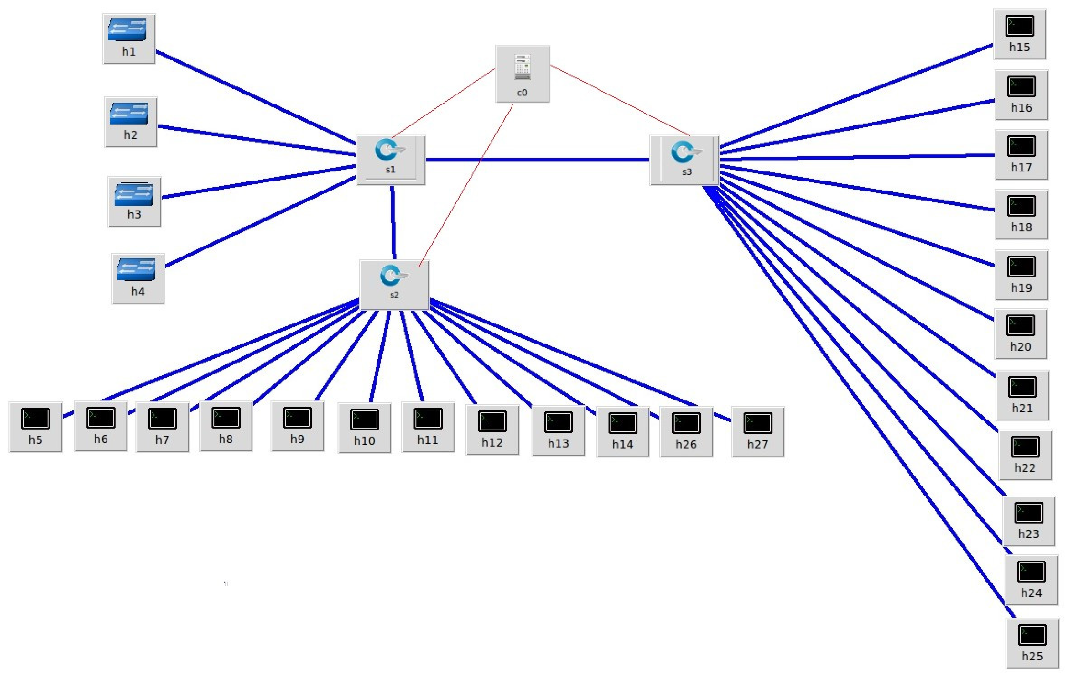
- (b)
- The network topology (shown in Figure 8) is drawn on the Mininet graphical interface or can be established by writing a command in the command line interface of Mininet.
- (c)
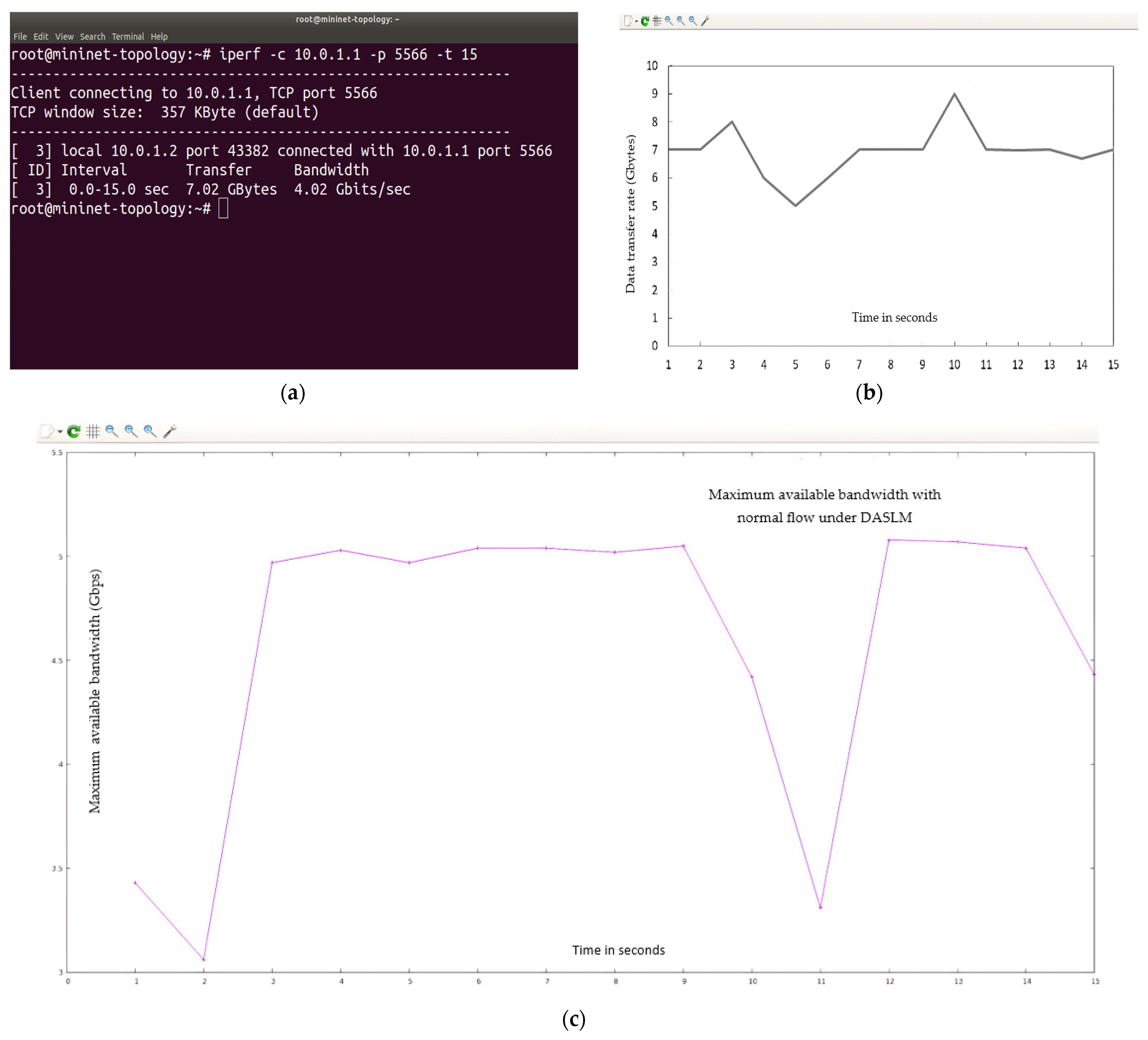
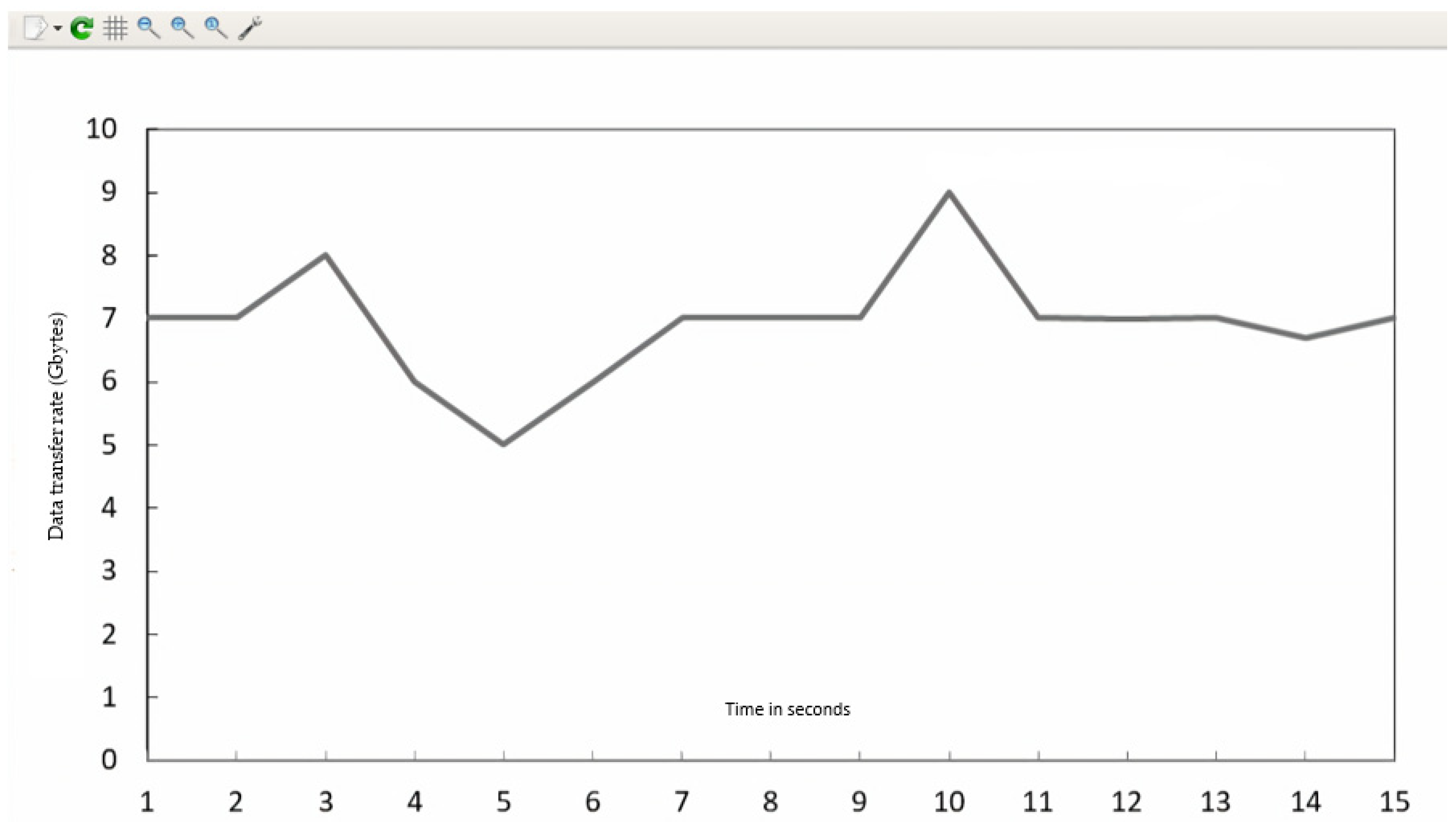
- Server load (in terms of HTTP requests) is calculated, and based on these calculations, the graph of the QoS parameters is obtained using the I-Perf and Gnu-plot utility.
- (a)
- The controller (POX) is switched to active mode by running the DASLM algorithm (with details as mentioned in Section 3.1).
- (b)
- The network topology (shown in Figure 8) is drawn on the Mininet graphical interface or can be established by writing a command in the command line interface of Mininet.
- (c)
- Server load (in terms of HTTP requests) is calculated, and based on these calculations, the graph of the QoS parameters is obtained using the I-Perf and Gnu-plot utility.
- (d)
- The comparison is drawn between the QoS parameters results obtained in both portions (1 and 2). However, the QoS parameter results in portion 2 will be far superior to those obtained in portion 1 (the QoS result details are explained in Section 4).
3.3. SDN-Based Environment (Lab Setup)
- (a)
- Two cores i-7 (HP 15 Dw4029NE, Core i7, 12th Generation, 256 GB SSD, 1 TB HDD, 2 GB NVIDIA MX550 DOS), ten generations with 32 GB RAM each.
- (b)
- With three VMs (virtual machines) on each PC, one is used to run an SDN controller, one for the Mininet topology, and the other for the network performance graph.
- (c)
- Mininet is required to simulate the network along the I-Perf and J-Perf (required for QOS parameter measurement).
- (d)
- P-J-T graph and Gnu-plot utility convert text files in the simulated graph for QOS parameter analysis.
- (e)
- Wireshark tool (for network graphs).
- (f)
- POX Controller (scripted in Python—version: 3.11.4).
4. Simulation Results and Discussion
4.1. (CaseI: Finding QoS Parameters of User-Defined Network Topology without the DASLM Algorithm)
4.1.1. Normal Flow
4.1.2. Loaded Scenario
4.2. Case II: Finding QoS Parameters of User-Defined Network Topology with the Implementation of the DASLM Algorithm on an SDN Controller
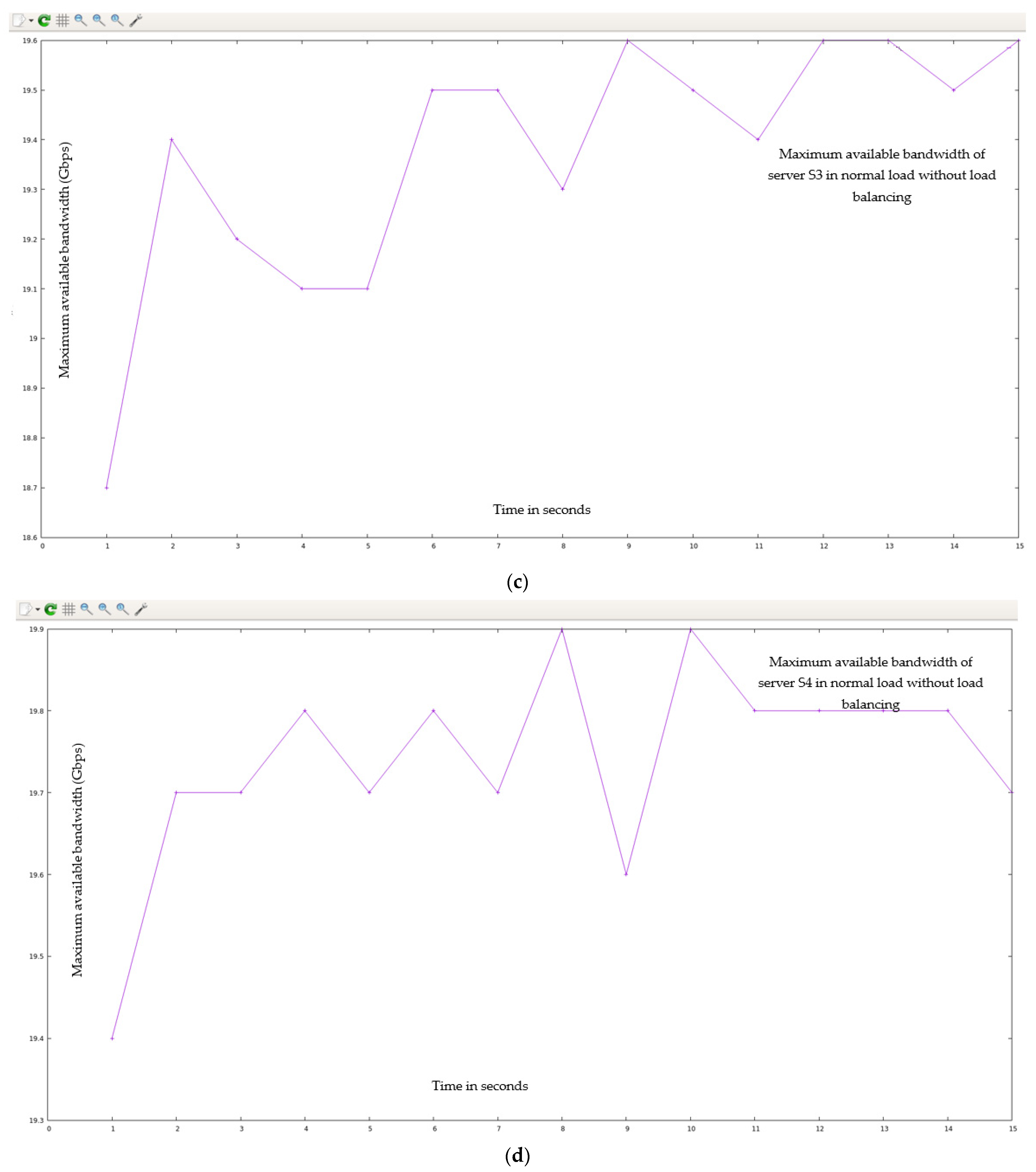
4.2.1. Normal Flow
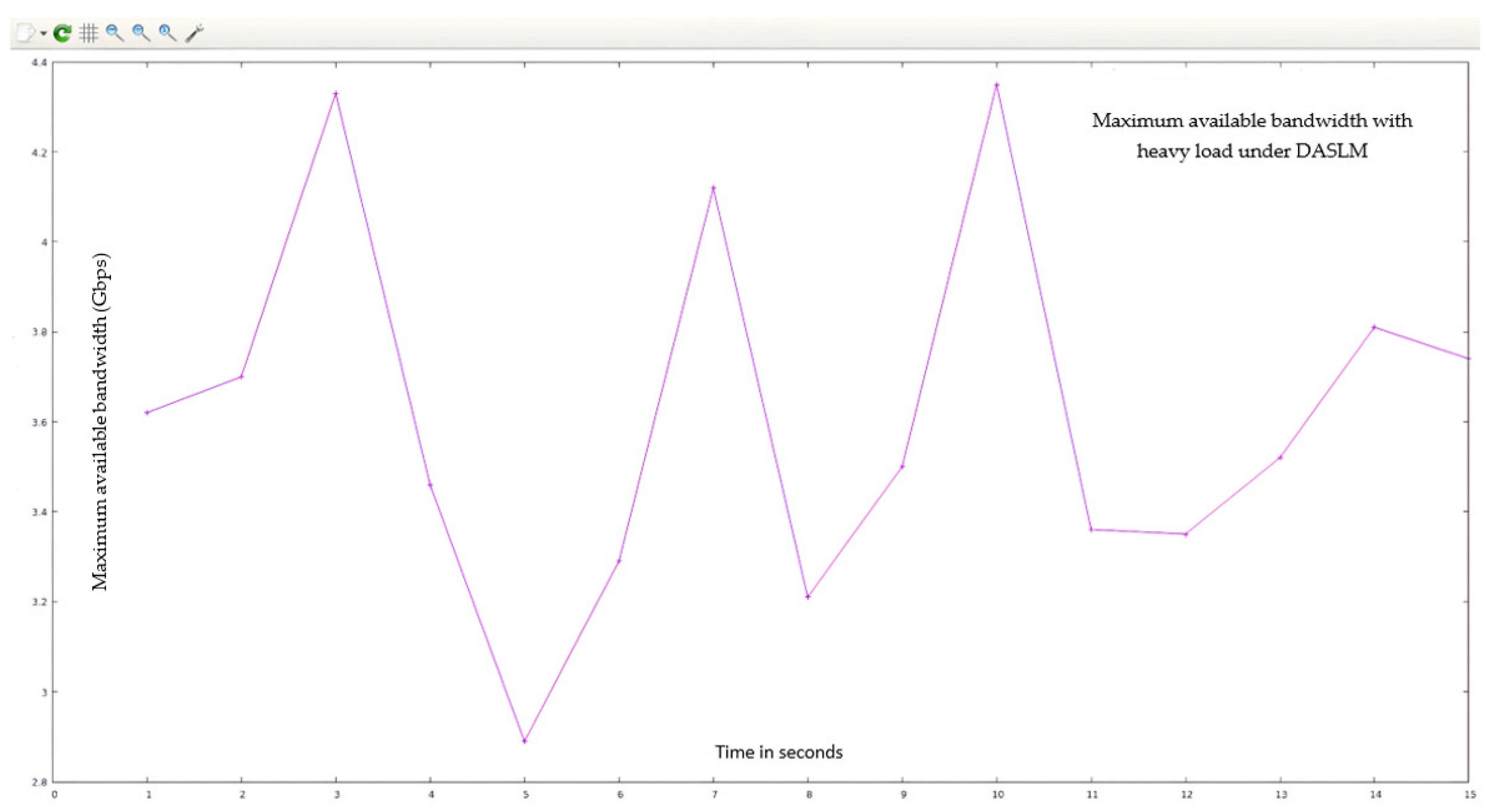
4.2.2. Loaded Scenario
4.3. Comparative Analysis of DASLM with Traditional Server Load-Balancing Methods
5. Conclusions
Author Contributions
Funding
Institutional Review Board Statement
Informed Consent Statement
Data Availability Statement
Conflicts of Interest
References
- Riyaz, M.; Musa, S. A Systematic Review of Load Balancing Technique in Software-Defined Networking. IEEE Access 2020, 8, 98612–98636. [Google Scholar]
- Liu, C.; Ju, W. An SDN-Based Active Measurement Method to Traffic QOS Sensing for Smart Network Access. Wirel. Netw. 2021, 27, 3677–3688. [Google Scholar] [CrossRef]
- Villalba, L.J.G.; Bi, J.; Jayasumana, A.P. Advances on Software Defined Sensor, Mobiles and Fixed Networks. Int. J. Distrib. Sens. Netw. 2016, 12, 5153718. [Google Scholar] [CrossRef]
- Ghalwash, H.; Huang, C. Software Defines Extreme Scale Networking for Big Data Applications. In Proceedings of the High-Performance Extreme Computing Conference (HPEC’17), Waltham, MA, USA, 12–14 September 2017. [Google Scholar]
- Andrus, B.; Olmos, J.J.V. SDN Data Center Performance Evaluation of Torus & Hypercube Inter-Connecting Schemes. In Proceedings of the Advances in Wireless and Optical Communication, Riga, Latvia, 5–6 November 2015; pp. 110–112. [Google Scholar]
- Gau, R.-H. Optimal Traffic Engineering and Placement of VM in SDN with Service Chaining. In Proceedings of the 2017 IEEE Conference on Network Softwarization (NetSoft), Bologna, Italy, 3–7 July 2017. [Google Scholar]
- Schwabe, A.; Rajos, E. Minimizing Downtime: Using Dynamic Reconfigurations and State Management in SDN. In Proceedings of the 2017 IEEE Conference on Network Softwarization (NetSoft), Bologna, Italy, 3–7 July 2017. [Google Scholar]
- Lin, C.; Wang, K. A QOS Aware Routing in SDN Hybrid Network. Procedia Comput. Sci. 2017, 110, 242–249. [Google Scholar] [CrossRef]
- Pasquini, R.; Stadler, R. Learning End-to-End Applications QOS from Open Flow Switch Statistics. In Proceedings of the 2017 IEEE Conference on Network Softwarization (NetSoft), Bologna, Italy, 3–7 July 2017. [Google Scholar]
- Zhang, T.; Liu, B. Exposing End-to-End Delay in SDN. Hindawi Int. J. Reconfigurable Comput. 2019, 2019, 7363901. [Google Scholar]
- Ghalwash, H.; Huang, C.-H. A QoS framework for SDN-Based Networking. In Proceedings of the 2018 IEEE 4th International Conference on Collaboration and Internet Computing (CIC), Philadelphia, PA, USA, 18–20 October 2018. [Google Scholar]
- Shu, Z.; Wan, J. Traffic Engineering in SDN: Measurement and Management. In IEEE Special Section on Green Communication and Networking for 5G Wireless; IEEE: Piscataway, NJ, USA, 2016; p. 6258274. [Google Scholar]
- Aly, W.H.F. Generic Controller Adaptive Load Balancing (GCALB) for SDN Networks. J. Comput. Netw. Commun. 2019, 2019, 6808693. [Google Scholar] [CrossRef]
- Xu, Y.; Cello, M.; Wang, I.-C.; Walid, A.; Wilfong, G.; Wen, C.H.-P.; Marchese, M.; Chao, H.J. Dynamic switch migration in distributed software-defined networks to achieve controller load balance. IEEE J. Sel. Areas Commun. 2019, 37, 515–529. [Google Scholar] [CrossRef]
- Gao, Y.; Zhang, Z.; Zhao, D.; Zhang, Y.; Luo, T. A hierarchical routing scheme with load balancing in software defined vehicular ad hoc networks. IEEE Access 2018, 6, 73774–73785. [Google Scholar] [CrossRef]
- Vyakaranal, S.B.; Naragund, J.G. Weighted round-robin load balancing algorithm for software-defined network. In Emerging Research in Electronics, Computer Science and Technology; Springer: Singapore, 2019; pp. 375–387. [Google Scholar]
- Tu, R.; Wang, X.; Zhao, J.; Yang, Y.; Shi, L.; Wolf, T. Design of a load-balancing middlebox based on SDN for data centers. In Proceedings of the 2015 IEEE Conference on Computer Communications Workshops (INFOCOM WKSHPS), Hong Kong, China, 26 April–1 May 2015; pp. 480–485. [Google Scholar]
- Hu, Y.; Luo, T.; Wang, W.; Deng, C. On the load balanced controller placement problem in software-defined networks. In Proceedings of the 2016 2nd IEEE International Conference on Computer and Communications (ICCC), Chengdu, China, 14–17 October 2016; pp. 2430–2434. [Google Scholar]
- Zhao, Y.; Liu, C.; Wang, H.; Fu, X.; Shao, Q.; Zhang, J. Load balancing-based multi-controller coordinated deployment strategy in software-defined optical networks. Opt. Fiber Technol. 2018, 46, 198–204. [Google Scholar] [CrossRef]
- Jiugen, S.; Wei, Z.; Kunying, J.; Ying, X. Multi-controller deployment algorithm based on load balance in a software-defined network. J. Electron. Inf. Technol. 2018, 40, 455–461. [Google Scholar]
- Wang, Q.; Gao, L.; Yang, Y.; Zhao, J.; Dou, T.; Fang, H. A Load-Balanced Algorithm for Multi-Controller Placement in a Software-Defined Network. Mech. Syst. Control Formerly Control Intell. Syst. 2018, 46, 72–81. [Google Scholar] [CrossRef]
- Ma, Y.-W.; Chen, J.-L.; Tsai, Y.-H.; Cheng, K.-H.; Hung, W.-C. Load-Balancing Multiple Controllers Mechanism for Software-Defined Networking. Wireless Pers. Commun. 2017, 94, 3549–3574. [Google Scholar] [CrossRef]
- Kaur, S.; Kumar, K.; Singh, J.; Ghumman, N.S. Round-Robin Based Load Balancing in Software-Defined Networking. In Proceedings of the 2nd International Conference on Computing for Sustainable Global DevelopmentAt: Bharati Vidyapeeth’s Institute of Computer Applications and Management (BVICAM), New Delhi, India, 11–13 March 2015; pp. 2136–2139. [Google Scholar]
- Mulla, M.M.; Raikar, M.; Meghana, M.; Shetti, N.S.; Madhu, R. Load Balancing for Software-Defined Networks. In Emerging Research in Electronics, Computer Science and Technology; Springer: Singapore, 2019; pp. 235–244. [Google Scholar]
- Chenhao, G.; Hengyang, W. An Improved Dynamic Smooth Weighted Round-robin Load-balancing Algorithm. In Journal of Physics: Conference Series, Proceedings of the 2nd International Conference on Electrical Engineering and Computer Technology (ICEECT 2022), Suzhou, China, 23–25 September 2022; IOP Publishing: Bristol, UK, 2022; Volume 2404, p. 2404. [Google Scholar]
- Al-Tam, F.; Correia, N. On Load Balancing via Switch Migration in Software-Defined Networking. IEEE Access 2019, 7, 95998–96010. [Google Scholar] [CrossRef]
- Linn, A.S.; Win, S.H.; Win, S.T. Server Load Balancing in Software Defined Networking. Natl. J. Parallel Soft Comput. 2019, 1, 261–265. [Google Scholar]
- Kaur, P.; Bhandari, A. A Comparison of Load Balancing Strategy in Software Defined Networking. Int. J. Res. Electron. Comput. Eng. IJRECE 2018, 6, 1018–1025. [Google Scholar]
- Yang, H.; Pan, H.; Ma, L. A Review on Software Defined Content Delivery Network: A Novel Combination of CDN and SDN. IEEE Access 2023, 11, 43822–43843. [Google Scholar] [CrossRef]
- Singh, I.T.; Singh, T.R.; Sina, T. Server Load Balancing with Round Robin Technique in SDN. In Proceedings of the 2022 International Conference on Decision Aid Sciences and Applications (DASA), Chiangrai, Thailand, 23–25 March 2022. [Google Scholar]
- Shona, M.; Sharma, R. Implementation and Comparative Analysis of Static and Dynamic Load Balancing Algorithms in SDN. In Proceedings of the 2023 International Conference for Advancement in Technology (ICONAT), Goa, India, 24–26 January 2023; pp. 1–7. [Google Scholar]
- Karnani, S.; Shakya, H.K. Leveraging SDN for Load Balancing on Campus Network (CN). In Proceedings of the 2021 13th International Conference on Computational Intelligence and Communication Networks (CICN), Lima, Peru, 22–23 September 2021; pp. 167–171. [Google Scholar]
- Sharma, R.; Reddy, H. Effect of Load Balancer on Software-Defined Networking (SDN) based Cloud. In Proceedings of the 2019 IEEE 16th India Council International Conference (INDICON), Rajkot, India, 13–15 December 2019. [Google Scholar]
- Huang, W.-Y.; Chou, T.-Y.; Hu, J.-W.; Liu, T.-L. Automatical End-to-End Topology Discovery and Flow Viewer on SDN. In Proceedings of the 2014 28th International Conference on Advanced Information Networking and Applications Workshops, Victoria, BC, Canada, 13–16 May 2014; pp. 910–915. [Google Scholar]
- Pakzad, F.; Portmann, M.; Tan, W.L.; Indulska, J. Efficient Topology Discovery in Software-Defined Networks. In Proceedings of the 2014 8th International Conference on Signal Processing and Communication Systems (ICSPCS), Gold Coast, QLD, Australia, 15–17 December 2014; pp. 1–8. [Google Scholar]
- Yuan, L.; Chuah, C.N.; Mohapatra, P. ProgME: Towards Pro-Programmable Network Measurement. IEEE/ACM Trans. Netw. 2011, 19, 115–128. [Google Scholar] [CrossRef]
- Tootoonchian, A.; Ghobadi, M.; Ganjali, Y. OpenTM: Traffic Matrix Estimator for OpenFlow Networks. In Passive and Active Measurement; Springer: Berlin/Heidelberg, Germany, 2010; pp. 201–210. [Google Scholar]
- Malboubi, M.; Wang, L.; Chuah, C.-N.; Sharma, P. Intelligent SDN Based Traffic (De) Aggregation and Measurement Paradigm (iSTAMP). In Proceedings of the IEEE INFOCOM 2014—IEEE Conference on Computer Communications, Toronto, ON, Canada, 27 April 2014–2 May 2014; pp. 934–942. [Google Scholar]
- Hu, Z.; Luo, J. Cracking Network Monitoring in DCNs with SDN. In Proceedings of the 2015 IEEE Conference on Computer Communications (INFOCOM), Hong Kong, China, 26 April 2015–1 May 2015; pp. 199–207. [Google Scholar]
- van Adrichem, N.L.M.; Doerr, C.; Kuipers, F.A. OpenNetMon: Network Monitoring in OpenFlow Software-Defined Networks. In Proceedings of the 2014 IEEE Network Operations and Management Symposium (NOMS), Krakow, Poland, 5–9 May 2014; pp. 1–8. [Google Scholar]
- Yu, C.; Lumezanu, C.; Zhang, Y.; Singh, V.; Jiang, G.; Madhyastha, H.V. FlowSense: Monitoring Network Utilization with Zero Measurement Cost. In PAM 2013: Passive and Active Measurement; Springer: Berlin/Heidelberg, Germany, 2013; Volume 7799, pp. 31–41. [Google Scholar]
- Mehmood, K.T.; Ateeq, S.; Hashmi, M.W. Predictive Analysis of Telecom System Quality Parameters with SDN (Software Define Networking) Controlled Environment. Ilkogr. Online-Elem. Educ. Online 2020, 19, 5562–5575. [Google Scholar]
- NetFlow. 2004. Available online: http://www.cisco.com/c/en/us/products/ios-nx-os-software/ios-netflow/index.html (accessed on 17 September 2004).
- sFlow. 2004. Available online: http://www.sflow.org/sFlowOverview.pdf (accessed on 1 July 2004).
- Myers, A.C. JFlow: Practical Mostly-Static Information Flow Control. In Proceedings of the 26th ACM SIGPLAN-SIGACT Symposium on Principles of Programming Languages, San Antonio, TX, USA, 20–22 January 1999; pp. 228–241. [Google Scholar]
- Chowdhury, S.; Bari, M.F.; Ahmed, R.; Boutaba, R. PayLess: A Low-Cost Network Monitoring Framework for Software-Defined Networks. In Proceedings of the 2014 IEEE Network Operations and Management Symposium (NOMS), Krakow, Poland, 5–9 May 2014; pp. 1–9. [Google Scholar]
- Yu, M.; Jose, L.; Miao, R. Software Defined Traffic Measurement with OpenSketch. In Proceedings of the 10th USENIX Symposium on Networked Systems Design and Implementation (NSDI 13), Lombard, IL, USA, 2–5 April 2013; pp. 29–42. [Google Scholar]
- Moshref, M.; Yu, M.; Govindan, R.; Vahdat, A. DREAM: Dynamic Resource Allocation for Software-Defined Measurement. In Proceedings of the SIGCOMM ‘14: Proceedings of the 2014 ACM Conference on SIGCOMM, Chicago, IL, USA, 17–22 August 2014. [Google Scholar]
- Mehdi, S.A.; Khalid, J.; Khayam, S.A. Revisiting Traffic Anomaly Detection Using Software-Defined Networking. In Proceedings of the RAID 2011: Recent Advances in Intrusion Detection, Menlo Park, CA, USA, 20–21 September 2011; pp. 161–180. [Google Scholar]
- Zuo, Q.; Chen, M.; Wang, X.; Liu, B. Online Traffic Anomaly Detection Method for SDN. J. Xidian Univ. 2015, 42, 155–160. (In Chinese) [Google Scholar]
- Canini, M.; Venzano, D.; Perešíni, P.; Kostić, D.; Rexford, J. A NICE Way to Test OpenFlow Applications. In Proceedings of the 9th USENIX Symposium on Networked Systems Design and Implementation (NSDI 12), San Jose, CA, USA, 25–27 April 2012; pp. 127–140. [Google Scholar]
- Khurshid, A.; Zou, X.; Zhou, W.; Caesar, M.; Godfrey, P. VeriFlow: Verifying Network-Wide Invariants in Real Time. In Proceedings of the SIGCOMM ‘12: ACM SIGCOMM 2012 Conference, Helsinki, Finland, 13 August 2012; pp. 15–27. [Google Scholar]
- Dixit, A.; Prakash, P.; Hu, Y.; Kompella, R. On the Impact of Packet Spraying in Data Center Networks. In Proceedings of the 2013 Proceedings IEEE INFOCOM, Turin, Italy, 14–19 April 2013; pp. 2130–2138. [Google Scholar]
- Chiesa, M.; Kindler, G.; Schapira, M. Traffic Engineering with Equal-Cost-Multipath: An Algorithmic Perspective. In Proceedings of the IEEE INFOCOM 2014—IEEE Conference on Computer Communications, Toronto, ON, Canada, 27 April–2 May 2014; pp. 1590–1598. [Google Scholar]
- Han, G.; Dong, Y.; Guo, H.; Shu, L.; Wu, D. Cross-Layer Optimized Routing in Wireless Sensor Networks with Duty Cycle and Energy Harvesting. Wireless Commun. Mobile Comput. 2015, 15, 1957–1981. [Google Scholar] [CrossRef]
- Chen, M.; Leung, V.C.M.; Mao, S.; Yuan, Y. Directional Geographical Routing for Real-Time Video Communications in Wireless Sensor Networks. Comput. Commun. 2007, 30, 3368–3383. [Google Scholar] [CrossRef]
- Chen, M.; Leung, V.C.M.; Mao, S.; Li, M. Cross-Layer and Path Priority Scheduling Based Real-Time Video Communications over Wireless Sensor Networks. In Proceedings of the VTC Spring 2008—IEEE Vehicular Technology Conference, Singapore, 11–14 May 2008; pp. 2873–2877. [Google Scholar]
- Al-Fares, M.; Radhakrishnan, S.; Raghavan, B.; Huang, N.; Vahdat, A. Hedera: Dynamic Flow Scheduling for Data Center Networks. In Proceedings of the NSDI’10: The 7th USENIX Conference on Networked Systems Design and Implementation, San Jose, CA, USA, 28–30 April 2010; Volume 10, p. 19. [Google Scholar]
- Curtis, A.R.; Kim, W.; Yalagandula, P. Mahout: Low-Overhead Data-Center Traffic Management Using End-Host-Based Elephant Detection. In Proceedings of the 2011 Proceedings IEEE INFOCOM, Shanghai, China, 10–15 April 2011; pp. 1629–1637. [Google Scholar]
- Benson, T.; Anand, A.; Akella, A.; Zhang, M. MicroTE: Fine-Grained Traffic Engineering for Data Centers. In Proceedings of the Co-NEXT ‘11: Conference on emerging Networking Experiments and Technologies, Tokyo, Japan, 6–9 December 2011; pp. 1–12. [Google Scholar]
- Curtis, A.R.; Mogul, J.C.; Tourrilhes, J.; Yalagandula, P.; Sharma, P.; Banerjee, S. DevoFlow: Scaling Flow Management for High-Performance Networks. ACM SIGCOMM Comput. Commun. Rev. 2011, 41, 254–265. [Google Scholar] [CrossRef]
- Yu, M.; Rexford, J.; Freedman, M.J.; Wang, J. Scalable Flow-Based Networking with DIFANE. SIGCOMM Comput. Commun. Rev. 2010, 40, 351–362. [Google Scholar] [CrossRef]
- Silva, T.; Arsenio, A. A Survey on Energy Efficiency for the Future Internet. Int. J. Comput. Commun. Eng. 2013, 2, 595–689. [Google Scholar] [CrossRef]
- Chen, M.; Zhang, Y.; Li, Y.; Mao, S.; Leung, V.C.M. EMC: Emotion-Aware Mobile Cloud Computing in 5G. IEEE Netw. 2015, 29, 32–38. [Google Scholar] [CrossRef]
- Ke, B.-Y.; Tien, P.-L.; Hsiao, Y.-L. Parallel Prioritized Flow Scheduling for Software-Defined Data Center Network. In Proceedings of the 2013 IEEE 14th International Conference on High Performance Switching and Routing (HPSR), Taipei, Taiwan, 8–11 July 2013; pp. 217–218. [Google Scholar]
- Li, D.; Shang, Y.; Chen, C. Software Defined Green Data Center Network with Exclusive Routing. In Proceedings of the IEEE INFOCOM 2014—IEEE Conference on Computer Communications, Toronto, ON, Canada, 27 April–2 May 2014; pp. 1743–1751. [Google Scholar]
- Amokrane, A.; Langar, R.; Boutabayz, R.; Pujolle, G. Online Flow-Based Energy Efficient Management in Wireless Mesh Networks. In Proceedings of the 2013 IEEE Global Communications Conference (GLOBECOM), Atlanta, GA, USA, 9–13 December 2013; pp. 329–335. [Google Scholar]
- Ali, S.; Alivi, M.K. Detecting DDoS Attack on SDN due to Vulnerabilities in OpenFlow. In Proceedings of the 2019 International Conference on Advances in the Emerging Computing Technologies (AECT), Al Madinah Al Munawwarah, Saudi Arabia, 10 February 2020. [Google Scholar]
- Sathyanarayana, S.; Moh, M. Joint route-server load balancing in software defined networks using ant colony optimization. In Proceedings of the 2016 International Conference on High Performance Computing & Simulation (HPCS), Innsbruck, Austria, 18–22 July 2016; pp. 156–163. [Google Scholar]
- Zhong, H.; Fang, Y.; Cui, J. Reprint of ‘LBBSRT’: “An efficient SDN load balancing scheme based on server response time”. Future Gener. Comput. Syst. 2018, 80, 409–416. [Google Scholar] [CrossRef]
- Hamed, M.; Elhalawany, B.; Fouda, M. Performance analysis of applying load balancing strategies on different SDN environments. Benha J. Appl. Sci. (BJSA) 2017, 2, 91–97. [Google Scholar] [CrossRef]
- Arahunashi, A.; Vaidya, G.; Neethu, S.; Reddy, K.V. Implementation of Server Load Balancing Techniques Using Software-Defined Networking. In Proceedings of the 2018, 3rd International Conference on Computational Systems and Information Technology for Sustainable Solutions(CSITSS), Bengaluru, India, 20–22 December 2018; pp. 87–90. [Google Scholar]
- Kaur, S.; Singh, J. Implementation of server load balancing in software defined networking. In Information Systems Design and Intelligent Applications; Springer: Berlin/Heidelberg, Germany, 2016; pp. 147–157. [Google Scholar]
- Kavana, H.; Kavya, V.; Madhura, B.; Kamat, N. Load balancing using SDN methodology. Int. J. Eng. Res. Technol. 2018, 7, 206–208. [Google Scholar]
- Hamed, M.; ElHalawany, B.M.; Fouda, M.M.; Eldien, A.S.T. A new approach for server-based load balancing using software-defined networking. In Proceedings of the 2017 Eighth International Conference on Intelligent Computing and Information Systems(ICICIS), Cairo, Egypt, 5–7 December 2017; pp. 30–35. [Google Scholar]
- Ejaz, S.; Iqbal, Z.; Shah, P.A.; Bukhari, B.H.; Ali, A.; Aadil, F. Traffic load balancing using software defined networking (SDN) controller as virtualized network function. IEEE Access 2019, 7, 46646–46658. [Google Scholar] [CrossRef]
- Gasmelseed, H.; Ramar, R. Traffic pattern-based load-balancing algorithm in software-defined network using distributed controllers. Int. J. Commun. Syst. 2019, 32, e3841. [Google Scholar] [CrossRef]
- Hai, N.T.; Kim, D.-S. Efficient load balancing for multi-controller in SDN-based mission-critical networks. In Proceedings of the 2016 IEEE 14th International Conference on Industrial Informatics (INDIN), Poitiers, France, 19–21 July 2016; pp. 420–425. [Google Scholar]
- Chiang, M.; Cheng, H.; Liu, H.; Chiang, C. SDN-based server clusters with dynamic load balancing and performance improvement. Clust. Comput. 2021, 24, 537–558. [Google Scholar] [CrossRef]
- Zhang, H.; Guo, X. SDN-based load balancing strategy for server cluster. In Proceedings of the 2014 IEEE 3rd International Conference on Cloud Computing and Intelligence Systems, Shenzhen, China, 27–29 November 2014. [Google Scholar]
- Kreutz, D.; Ramos, F.M.V.; Verissimo, P. Towards secure and dependable software-defined networks. In Proceedings of the HotSDN ‘13: The Second ACM SIGCOMM Workshop on Hot Topics in Software Defined Networking, Hong Kong, China, 16 August 2013; pp. 55–60. [Google Scholar]
- Yeganeh, S.H.; Tootoonchian, A.; Ganjali, Y. On scalability of software-defined networking. IEEE Commun. Mag. 2013, 51, 136–141. [Google Scholar] [CrossRef]
- Gude, N.; Koponen, T.; Pettit, J.; Pfaff, B.; Casado, M.; McKeown, N.; Shenker, S. NOX: Towards an operating system for networks. ACM SIGCOMM Comput. Commun. Rev. 2008, 38, 105–110. [Google Scholar] [CrossRef]
- Sezer, S.; Scott-Hayward, S.; Chouhan, P.; Fraser, B.; Lake, D.; Finnegan, J.; Viljoen, N.; Miller, M.; Rao, N. Are we ready for SDN? Implementation challenges for software-defined networks. IEEE Commun. Mag. 2013, 51, 36–43. [Google Scholar] [CrossRef]
- Karakus, M.; Durresi, A. A survey: Control plane scalability issues and approaches in software-defined networking (SDN). Comput. Netw. 2017, 112, 279–293. [Google Scholar] [CrossRef]


| References | Improvement in Network with the Author’s Technique | Limitation | Comparison with the Proposed Algorithm (DASLM) |
|---|---|---|---|
| S. Sathyanarayana et al. [69] | The authors combine the ant colony algorithm with the dynamic flow algorithm. The less-loaded server is found with the dynamic flow algorithm, and the shortest path to the less-loaded server is found using the ant algorithm technique. | In this paper, the latency is reduced. However, combining two algorithms and running them simultaneously extensively uses computer resources, memory, and bandwidth. | The proposed algorithm (DASLM) is a single active sensing dynamic algorithm that balances the load on HTTP servers in the SDN network by calculating their HTTP request load. If the HTTP request load of any server exceeds the range of the server load threshold (SLT) value, the load is shifted to the server with less HTTP request load. However, if the above condition is not met, HTTP requests are forwarded to the server with a quicker response time. As a result, the transfer rate, available bandwidth, and throughput are increased, and there are no overhead issues. |
| H. Zhong et al. [70] | In this research paper, the HTTP request flow is managed based on server response time calculations. | Processing delays are reduced only. | The proposed algorithm (DASLM) not only balances the load on HTTP servers in the SDN network by calculating the response time by sending ARP packets but also selects the optimum server by (a) calculating RPS and comparing the RPS value with the reference threshold SLT value and (b) finding the number of HTTP requests in the queue to be processed by the respective servers of the SDN network. |
| Hamed et al. [71] | The (HTTP request) load among different servers is balanced using the traditional Round-Robin method. | This method is simple and easy to implement and distributes the HTTP request load among different servers in sequential order. This method has greater limitations in large SDN networks with heavy data flow. | The proposed algorithm (DASLM) is more advanced than the method adopted for load balance [52]. In the proposed method, the optimum server for better managing HTTP request flow is selected based on response time calculation, calculation of RPS and comparison with threshold SLT value, and finding the number of HTTP requests in the queue of respective servers to be processed. |
| Arahunashi et al. [72] | The (HTTP request) load among different servers is balanced by calculating each server’s maximum available bandwidth. | The throughput and response time calculation is not considered. | The DASLM algorithm performs load balancing among different available servers based on (a) maximum available bandwidth (by calculating the server load), (b)response time, and (c) processing delays. |
| Kaur et al. [73] | The authors use a direct routing algorithm that directs the server’s response to the host without passing through the load balancer. With this method, the author has claimed a decrease in latency. | The flow control is very much compromised. | In the DASLM algorithm, the RPS value of each server for every flow is calculated, and then, based on comparisons with SLT value, the load is shared among different servers. |
| Kavana et al. [74] | The authors use a flood light controller, and the link path cost calculation is performed with the shortest path first. | HTTP request load is balanced among different available servers based on link cost optimization and no real-time traffic flow sensing. | DASLM performs real-time HTTP request flow sensing and distributes the HTTP request load among different available servers based on calculations performed for every flow. |
| Hamed et al. [75] | Comparison of Raspberry-Pi-based network and the network formed on Mininet. | The result claimed by the authors is that the SDN-based network has better performance in server load balancing. | The DASLM is implemented in a Mininet environment with a POX controller. |
| S. Ejaz et al. [76] | The authors propose using two controllers (master and slave). All copies of files regarding flow management in the network are saved on the master controller so that if the controller fails, other controllers manage the flow. | A logically centralized environment requires tight synchronization. | DASLM proposes the use of a logically distributed environment. |
| H.Gasmelseed et al. [77] | In this study, the authors propose the use of two controllers. One controller controls the TCP flow, while the other manages the UDP flow and shares files at the end of every flow so that if the controller fails, other controllers manage the flow. | A logically centralized environment requires tight synchronization. | DASLM proposes the use of a logically distributed environment. In this arrangement, every controller manages the flow of their subdivided network. |
| N.T. Hai et al. [78] | The data traffic is distributed into two categories: (1) critical time traffic and (2) non-critical time traffic, and in the case of congestion, the critical time traffic is given priority. | Minimized data transmission with a greater packet drop ratio. | In the DASLM algorithm, every traffic flow is given equal importance, and real-time HTTP request load calculations manage the flow. |
| M.L.Chiang et al. [79] | In this research article, the authors use a flood light controller with dynamic load balancing to reach the under-utilized server among different servers available in the network. The HTTP request load is shifted to the server with less RPS (HTTP request per second) load. | No work is conducted regarding response time. | The DASLM algorithm has the advanced feature of computing the server response time and finding the number of HTTP requests in the queue to be processed by the respective server. |
| H.Zhong et al. [80] | This paper draws a comparison between static and dynamic scheduling algorithms. | The dynamic scheduling algorithm has better flow characteristics. | DASLM is the active sensing load-balancing algorithm that performs real-time calculations to distribute the HTTP request load uniformly among network servers. |
| Load Testing | Time | Bam | Th | Tf (in 15 s) |
|---|---|---|---|---|
| Test #4 (with 1000 HTTP requests per second) | 0–15 s | 3.48 Gbps | 3.23 Gbps | 6.07 Gbytes |
| Test #3 (with 3750 HTTP requests per second) | 0–15 s | 2.10 Gbps | 2.29 Gbps | 4.298 Gbytes |
| Test #2 (with 3000 HTTP requests per second) | 0–15 s | 2.50 Gbps | 2.44 Gbps | 4.587 Gbytes |
| Test #1 (with 2000 HTTP requests per second) | 0–15 s | 3.17 Gbps | 3.14 Gbps | 5.897 Gbytes |
| Parameters | Descriptions | Values |
|---|---|---|
| T in sec | Total simulation time in sec | 0–15 |
| Bam | Maximum available bandwidth in Gbps | Value to be calculated by I-Perf utility during both cases: (1) normal flow and (2) loaded flow |
| Th | Throughput in Gbps | Value to be calculated by I-Perf utility during both cases: (1) normal flow and (2) loaded flow |
| Tf | Transfer rate in G-bytes | Value to be calculated by I-Perf utility during both cases: (1) normal flow and (2) loaded flow |
| SLT value | Server load threshold value | 1000 (RPS) is chosen as the reference value to compute the server load |
| L | Latency in ms | Value to be calculated by I-Perf utility during both cases: (1) normal flow and (2) loaded flow |
| RPS | Requests per second | 150 RPS during case (1) normal flow and 15,000 during case (2) loaded flow |
| %TF | Percentage decrease in transfer rate | Value to be calculated by I-Perf utility during both cases: (1) normal flow and (2) loaded flow |
| %L | Percentage increase in server load | Value to be calculated by I-Perf utility during both cases: (1) normal flow and (2) loaded flow |
| % Bmax | Maximum available bandwidth percentage | Value to be calculated by I-Perf utility during both cases: (1) normal flow and (2) loaded flow |
| %Taf | Achievable transfer rate percentage | Value to be calculated by I-Perf utility during both cases: (1) normal flow and (2) loaded flow |
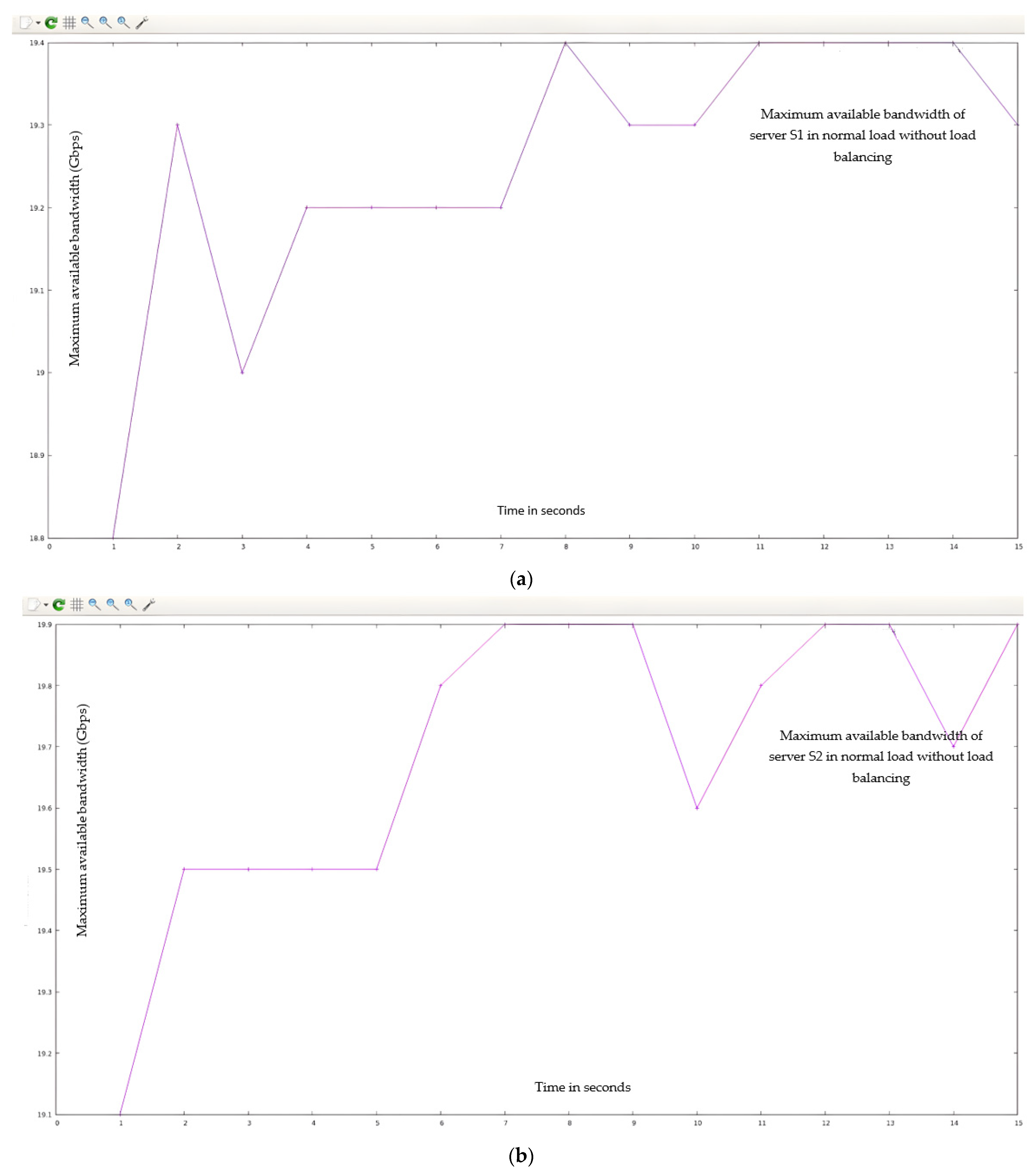
| List of HTTP Servers | Time in s | Bam | Th | Tf (in 15 s) |
|---|---|---|---|---|
| Server#1 | 0–15 s | 19.3 Gbps | 17.92 Gbps | 33.6 Gbytes |
| Server#2 | 0–15 s | 19.7 Gbps | 18.34 Gbps | 34.4 Gbytes |
| Server#3 | 0–15 s | 19.4 Gbps | 18.0266 Gbps | 33.8 Gbytes |
| Server#4 | 0–15 s | 19.7 Gbps | 18.4 Gbps | 34.5 Gbytes |
| List of HTTP Servers | Time | Bam | Th | Tf (in 15 s) | 156 Packets Tavr (ms) | L (ms) | %Tf | %L |
|---|---|---|---|---|---|---|---|---|
| S2 (Normal Flow) | 0–15 s | 19.7 Gbps | 18.34 Gbps | 34.4 Gbytes | 155,790.81 | 0.299 | X | X |
| S2 (Loaded Scenario) | 0–15 s | 943 Mbps | 0.88 Gbps | 1.65 Gbytes | 156,765 | 12 | 95.43% | 95% |
| Interface | Time in s | Bam | Th | Tf (in 15 s) |
|---|---|---|---|---|
| The link between the controller and the HTTP request generator virtual machine | 0–15 s | 4.02 Gbps | 3.744 Gbps | 7.02 Gbytes |
| Interface/Servers | Time | Bam | Th | Tf (in 15 s) | Available Bandwidth Percentage | Achievable Transfer Rate (%) | 156 Packets Tavr (ms) | L (ms) | %Tf | %L |
|---|---|---|---|---|---|---|---|---|---|---|
| (Normal Flow) with DASLM | 0–15 s | 4.02 Gbps | 3.744 Gbps | 7.02 Gbytes | X | X | 790.81 | 0.2 | X | X |
| (Loaded Scenario) with DASLM | 0–15 s | 3.48 Gbps | 3.23 Gbps | 6.07 Gbytes | 86.57% | 86.47% | 865.67 | 0.87 | 13.53% | 13.43% |
| (Loaded Scenario) without DASLM | 0–15 s | 943 Mbps | 0.88 Gbps | 1.65 Gbytes | 4.78% | 4.65% | 156,765 | 12 | 95.43% | 95% |
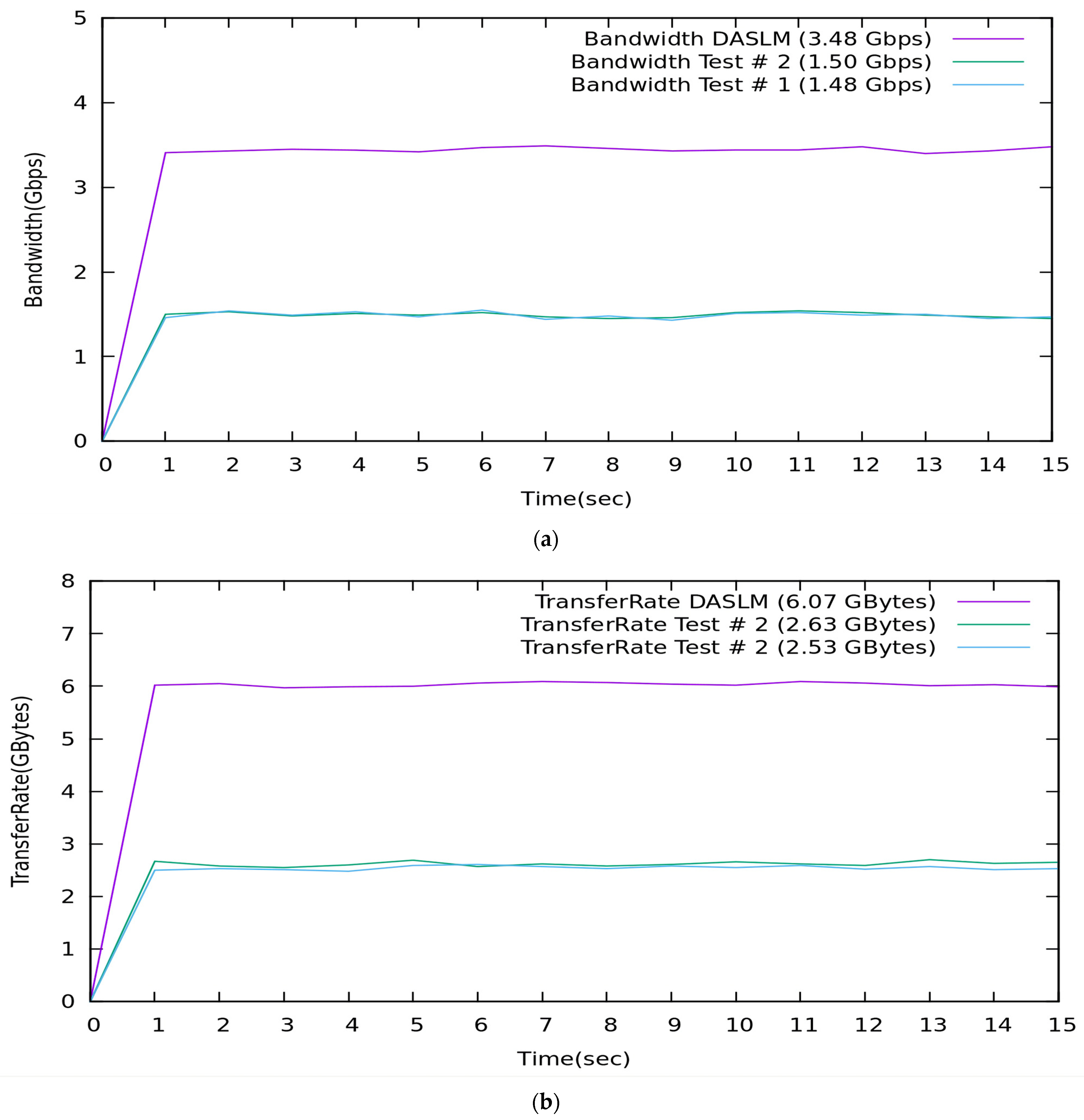
| Method Used | Time | Bam | Th | Tf (in 15 s) |
|---|---|---|---|---|
| QoS parameters with DASLM Algorithm. | 0–15 s | 3.48 Gbps | 3.23 Gbps | 6.07 Gbytes |
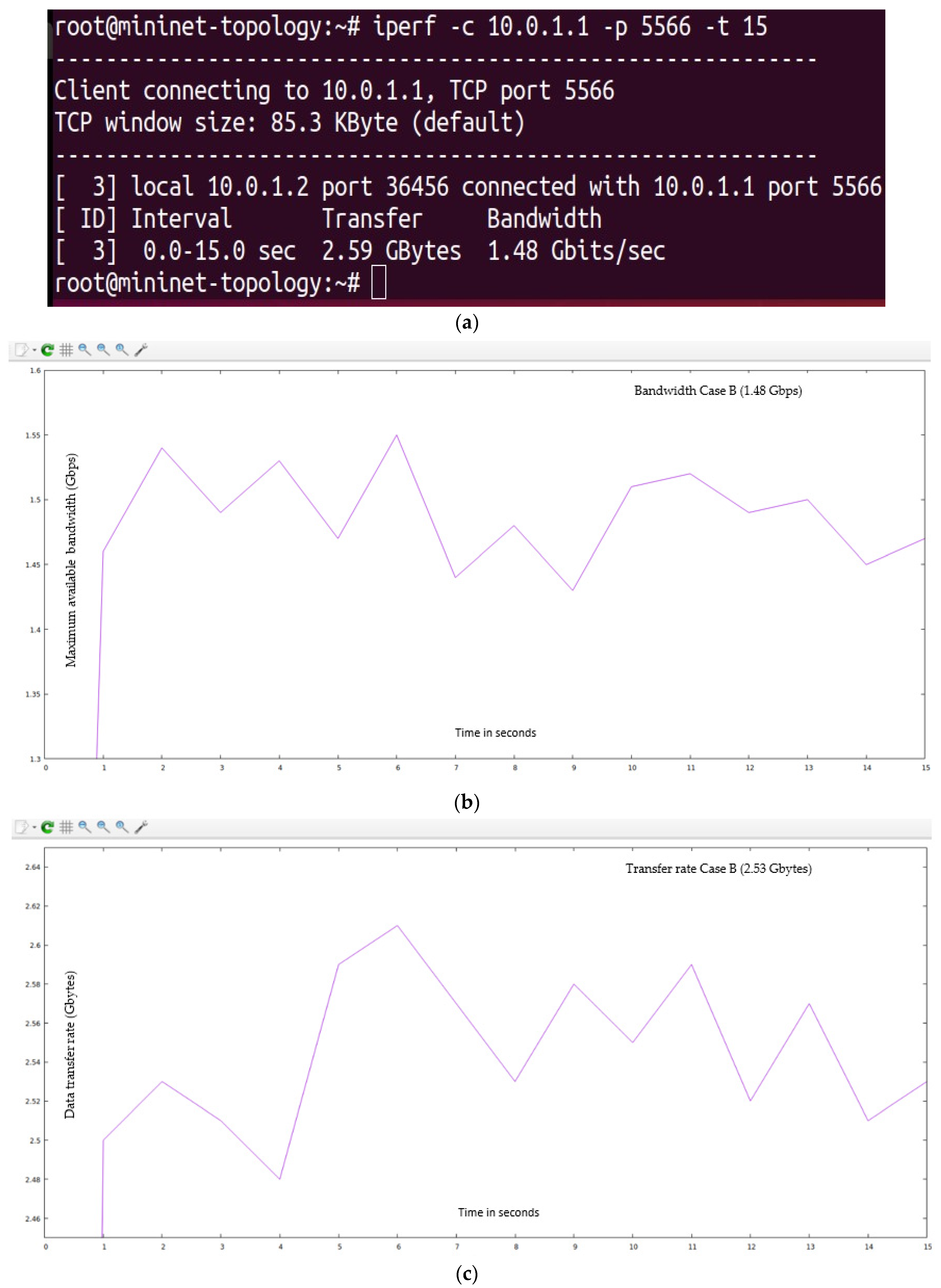
| Case B | 0–15 s | 1.48 Gbps | 1.38 Gbps | 2.59 Gbytes |
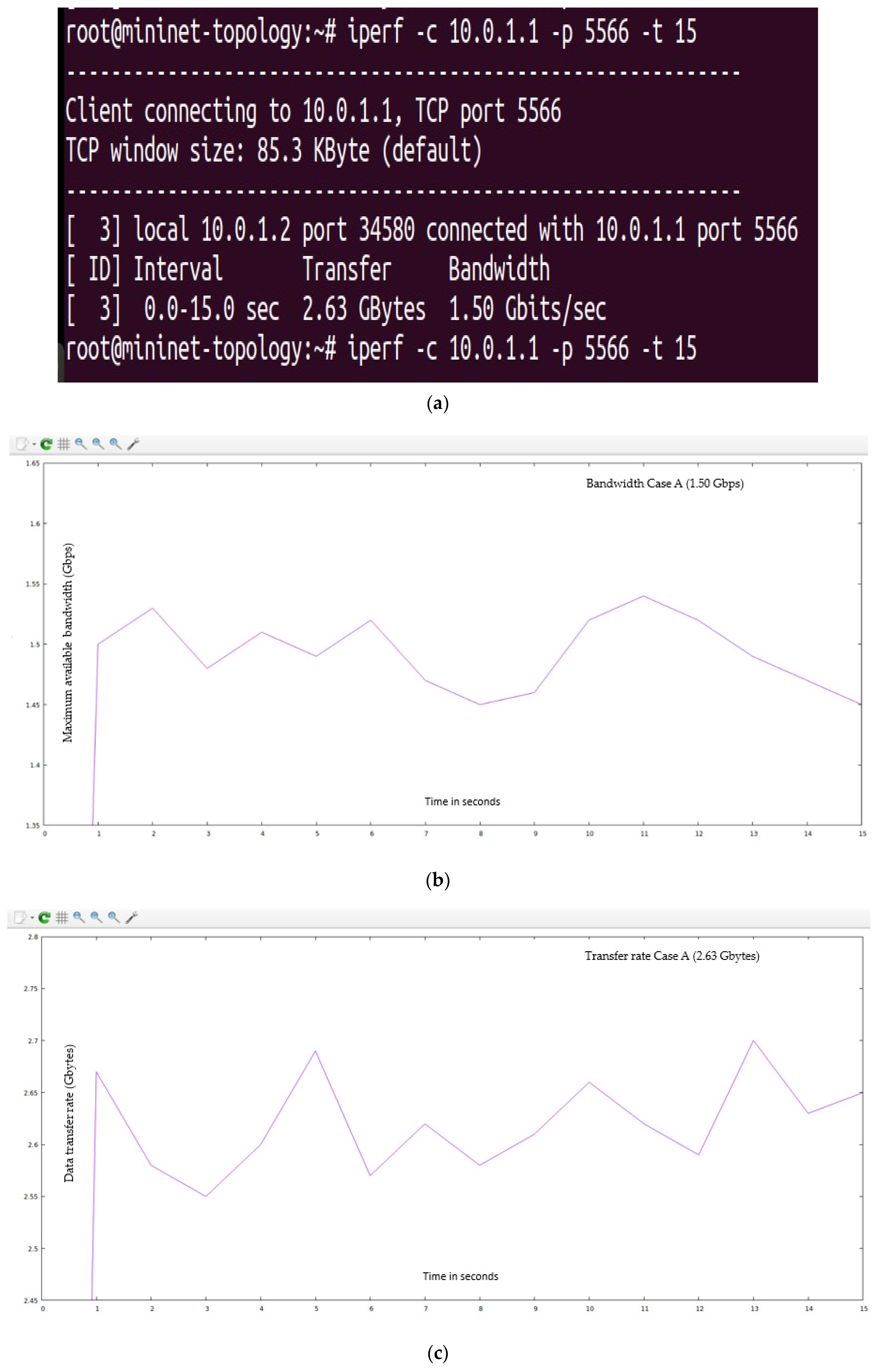
| Case A | 0–15 s | 1.50 Gbps | 1.40 Gbps | 2.63 Gbytes |
Disclaimer/Publisher’s Note: The statements, opinions and data contained in all publications are solely those of the individual author(s) and contributor(s) and not of MDPI and/or the editor(s). MDPI and/or the editor(s) disclaim responsibility for any injury to people or property resulting from any ideas, methods, instructions or products referred to in the content. |
© 2023 by the authors. Licensee MDPI, Basel, Switzerland. This article is an open access article distributed under the terms and conditions of the Creative Commons Attribution (CC BY) license (https://creativecommons.org/licenses/by/4.0/).
Share and Cite
Mehmood, K.T.; Atiq, S.; Hussain, M.M. Enhancing QoS of Telecom Networks through Server Load Management in Software-Defined Networking (SDN). Sensors 2023, 23, 9324. https://doi.org/10.3390/s23239324
Mehmood KT, Atiq S, Hussain MM. Enhancing QoS of Telecom Networks through Server Load Management in Software-Defined Networking (SDN). Sensors. 2023; 23(23):9324. https://doi.org/10.3390/s23239324
Chicago/Turabian StyleMehmood, Khawaja Tahir, Shahid Atiq, and Muhammad Majid Hussain. 2023. "Enhancing QoS of Telecom Networks through Server Load Management in Software-Defined Networking (SDN)" Sensors 23, no. 23: 9324. https://doi.org/10.3390/s23239324
APA StyleMehmood, K. T., Atiq, S., & Hussain, M. M. (2023). Enhancing QoS of Telecom Networks through Server Load Management in Software-Defined Networking (SDN). Sensors, 23(23), 9324. https://doi.org/10.3390/s23239324