
Forward Collision Warning Strategy Based on Millimeter-Wave Radar and Visual Fusion
Abstract
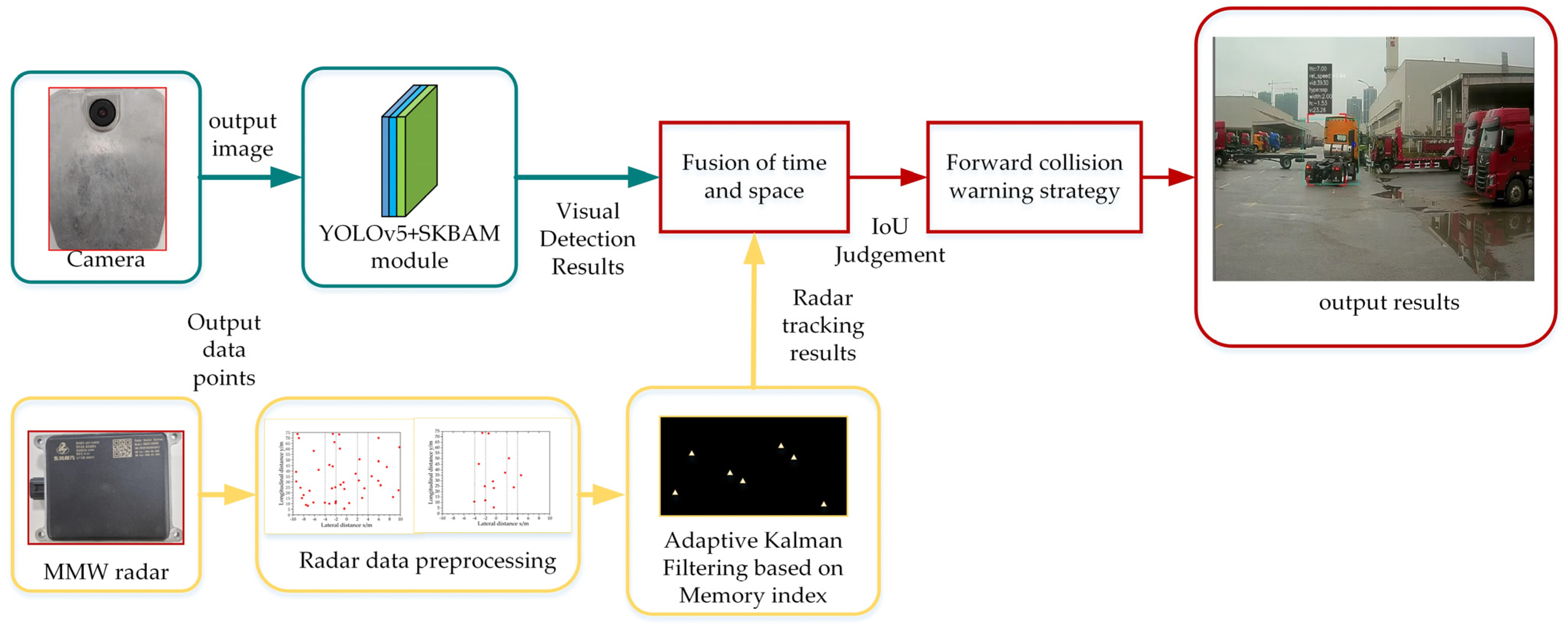
:1. Introduction
- According to the advantages of the existing advanced attention mechanism, this paper improves the CBAM attention mechanism (convolutional block attention module) and obtains a selective kernel and bottleneck attention mechanism (SKBAM). We add the SKBAM module to the network structure of the YOLOv5 algorithm model and verify the advantages of the improved YOLOv5 algorithm through an ablation experiment comparison.
- A memory index adaptive Kalman filter algorithm based on information entropy is proposed, which can adaptively adjust the noise covariance according to the system state and improve the accuracy of target tracking in millimeter-wave radar.
- A forward collision warning strategy for decision-level fusion of millimeter-wave radar and vision is designed. Experiments show that the strategy reduces the false alarm rate and missed alarm rate of the existing fusion algorithm in different environments and improves the accuracy of collision warning.
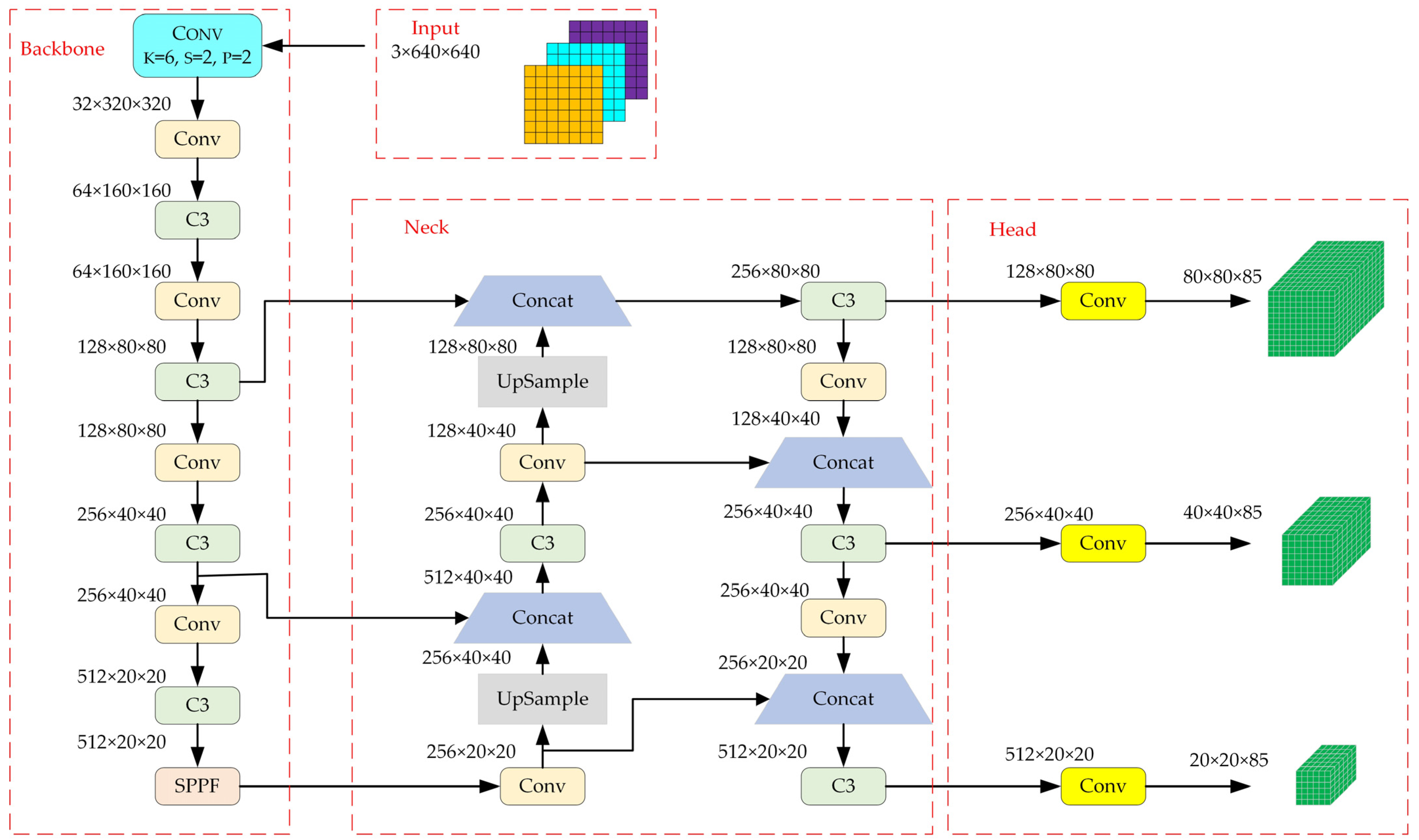
2. Visual Sensor Detection Model
2.1. YOLOv5 Visual Detection Model
2.2. Improved YOLOv5 Visual Detection Model
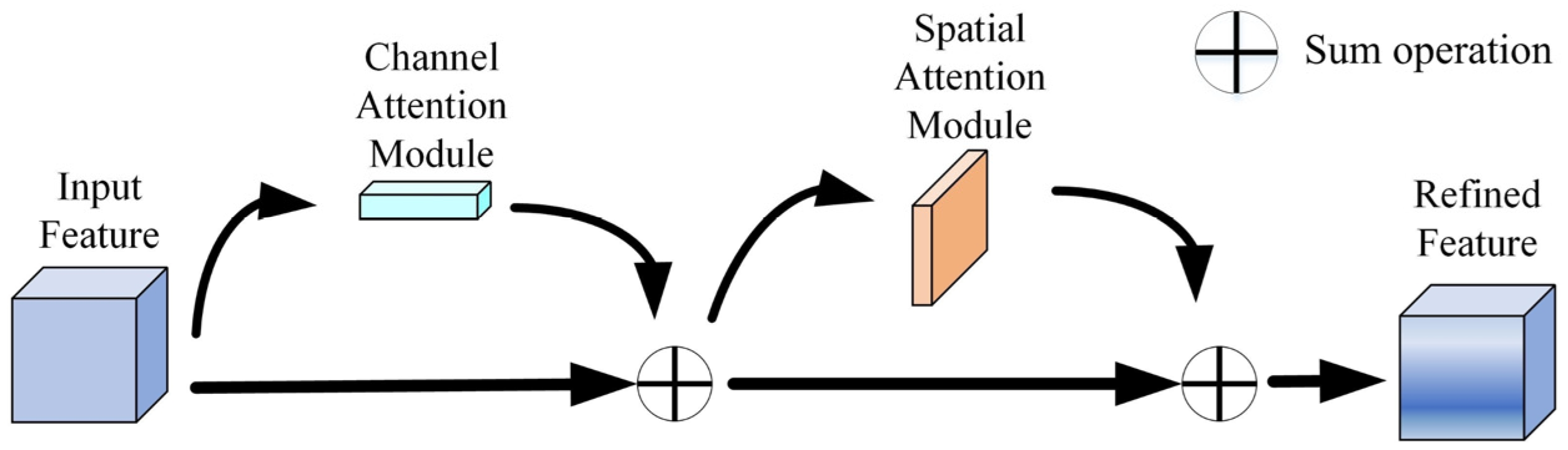
2.2.1. Attention Mechanism
2.2.2. Improved Channel Attention
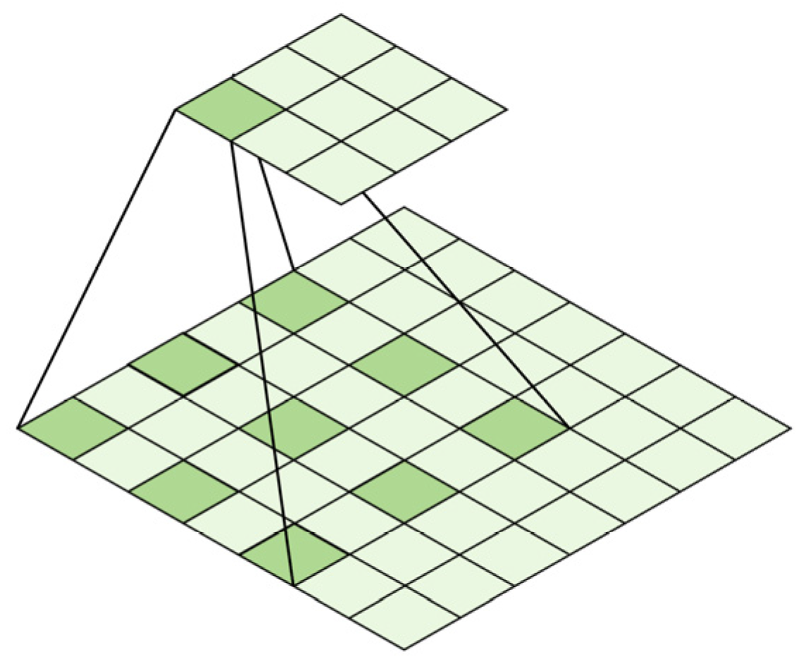
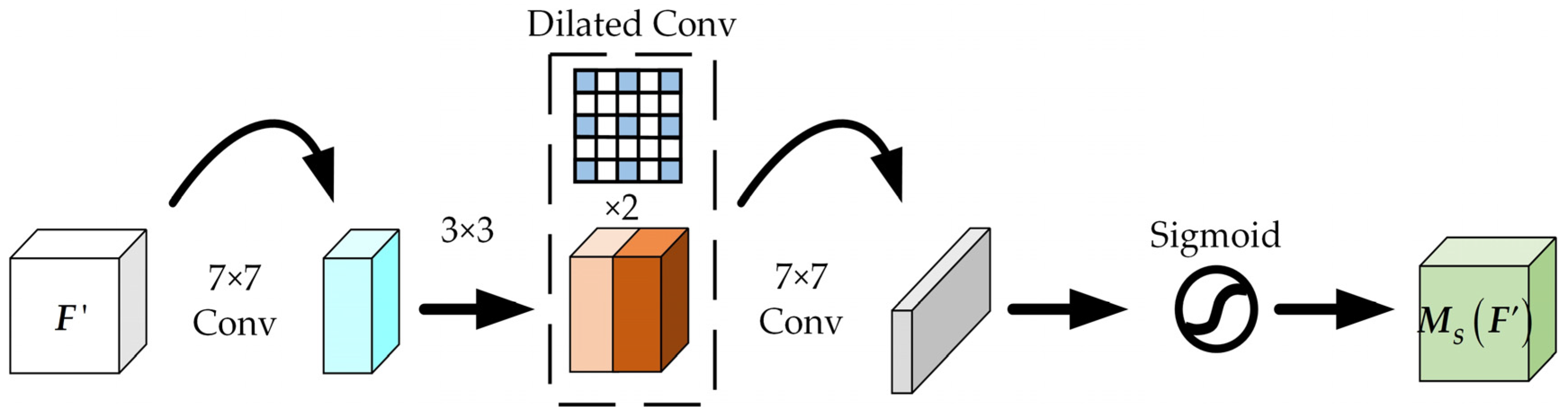
2.2.3. Improved Spatial Attention Submodule of CBAM
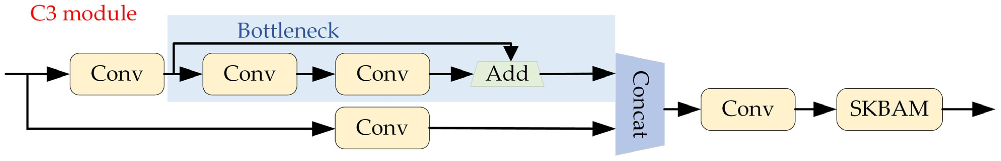
2.2.4. YOLOv5 Introduces SKBAM
3. Millimeter Wave Radar Detection Model
3.1. Radar Data Preprocessing
3.2. Adaptive Kalman Filtering Based on Memory Index
| Algorithm 1 Adaptive Kalman Filtering based on Memory index |
|
|
|
|
|
|
|
|
|
|
4. Collision Warning Strategy
4.1. Fusion of Sensors in Space and Time
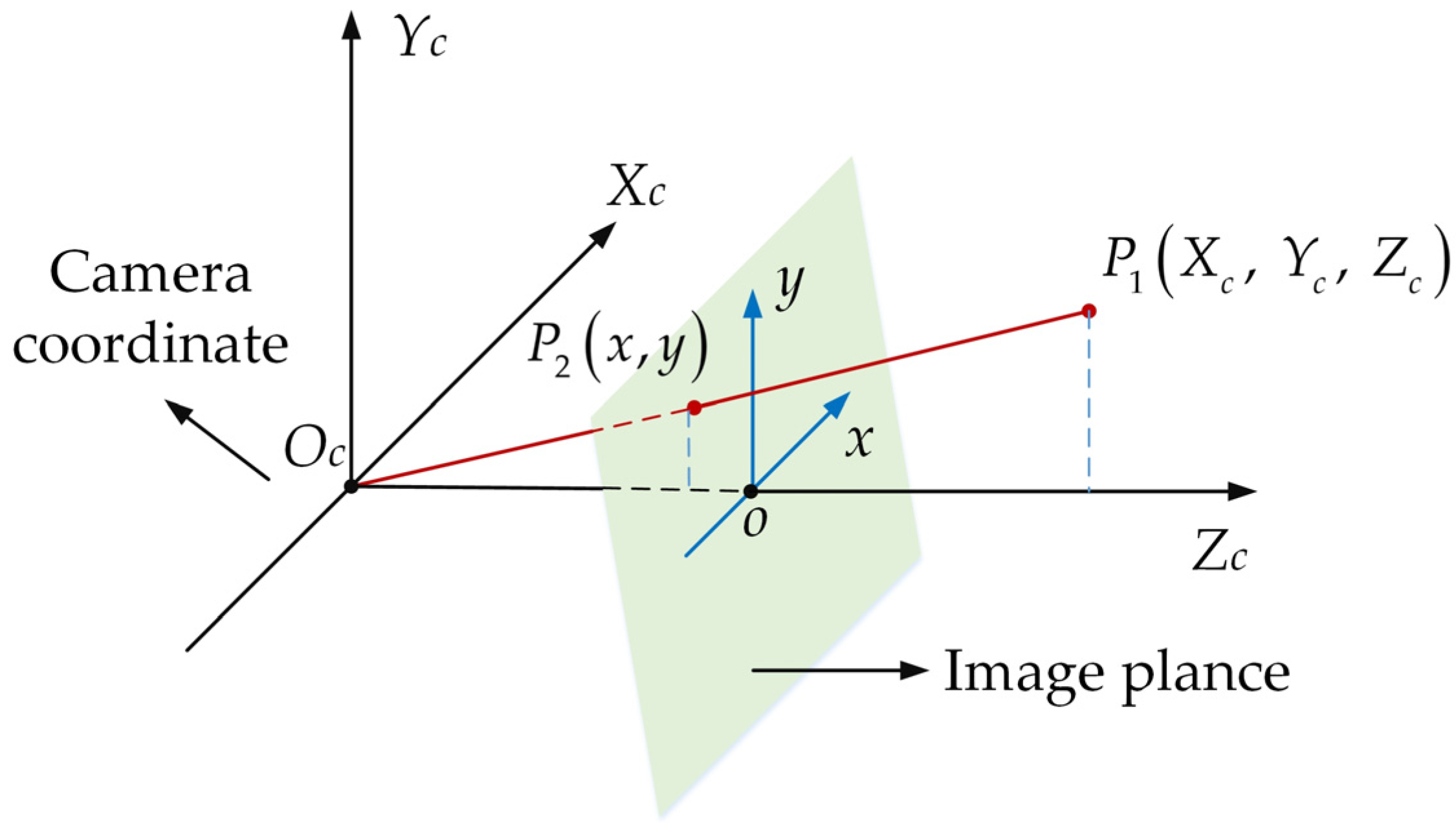
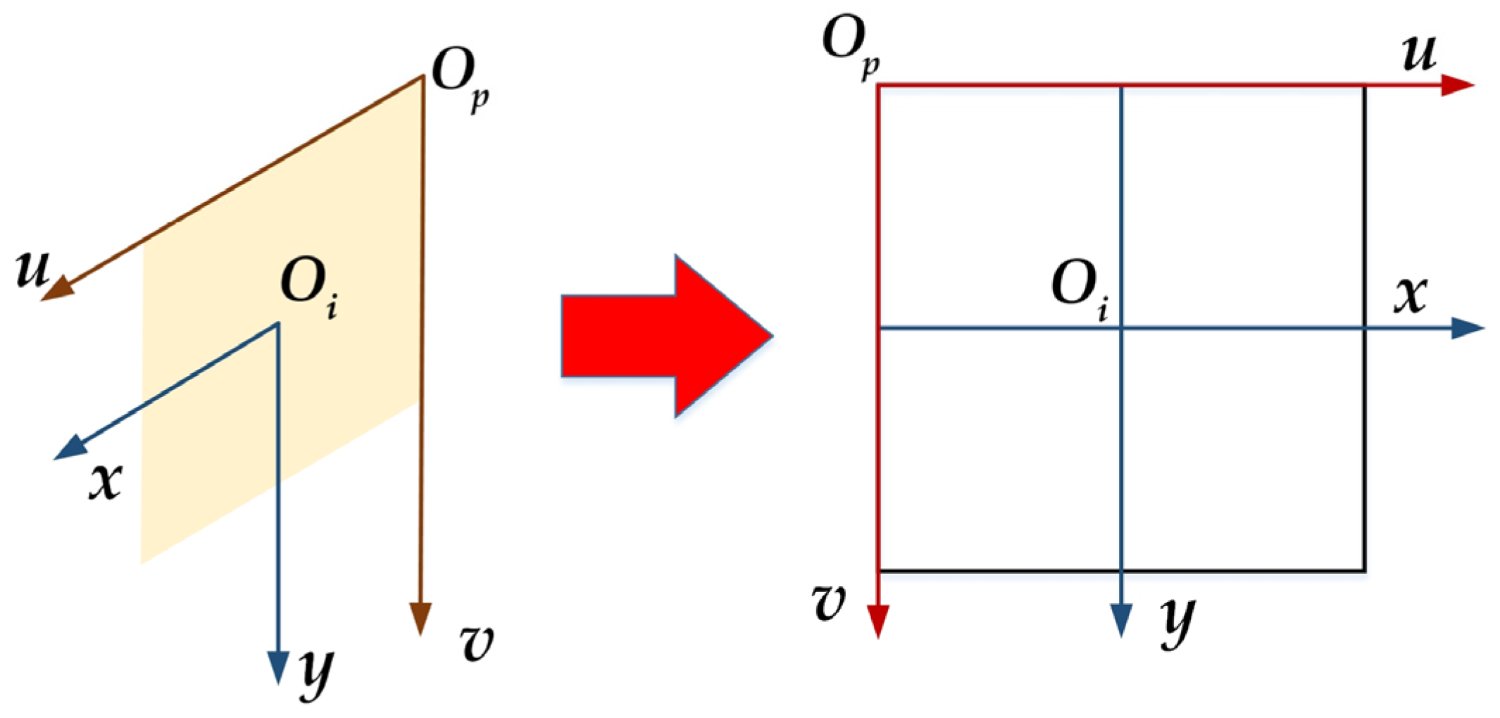
4.1.1. Spatial Fusion of Radar and Camera
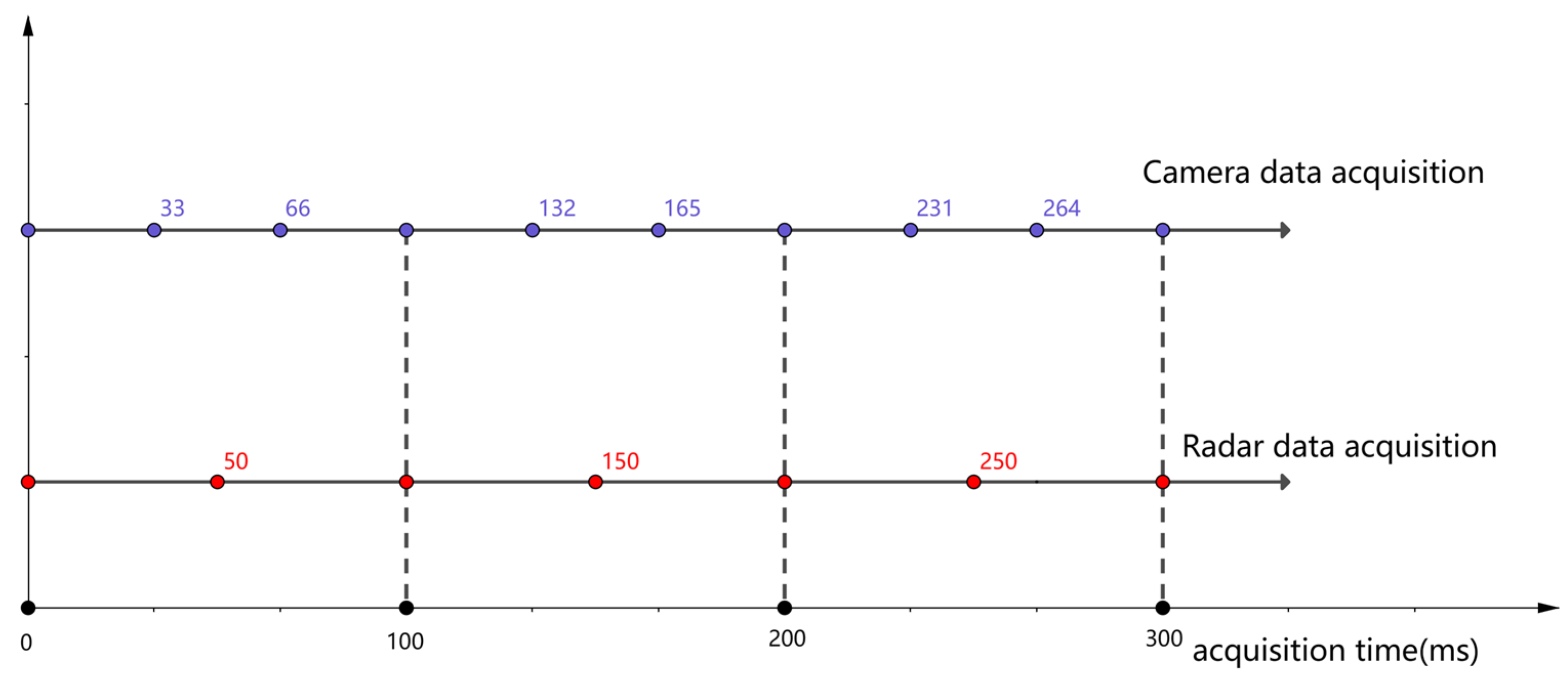
4.1.2. Time Fusion of Radar and Camera
4.2. Decision Level Fusion with Intersection over Union Ratio
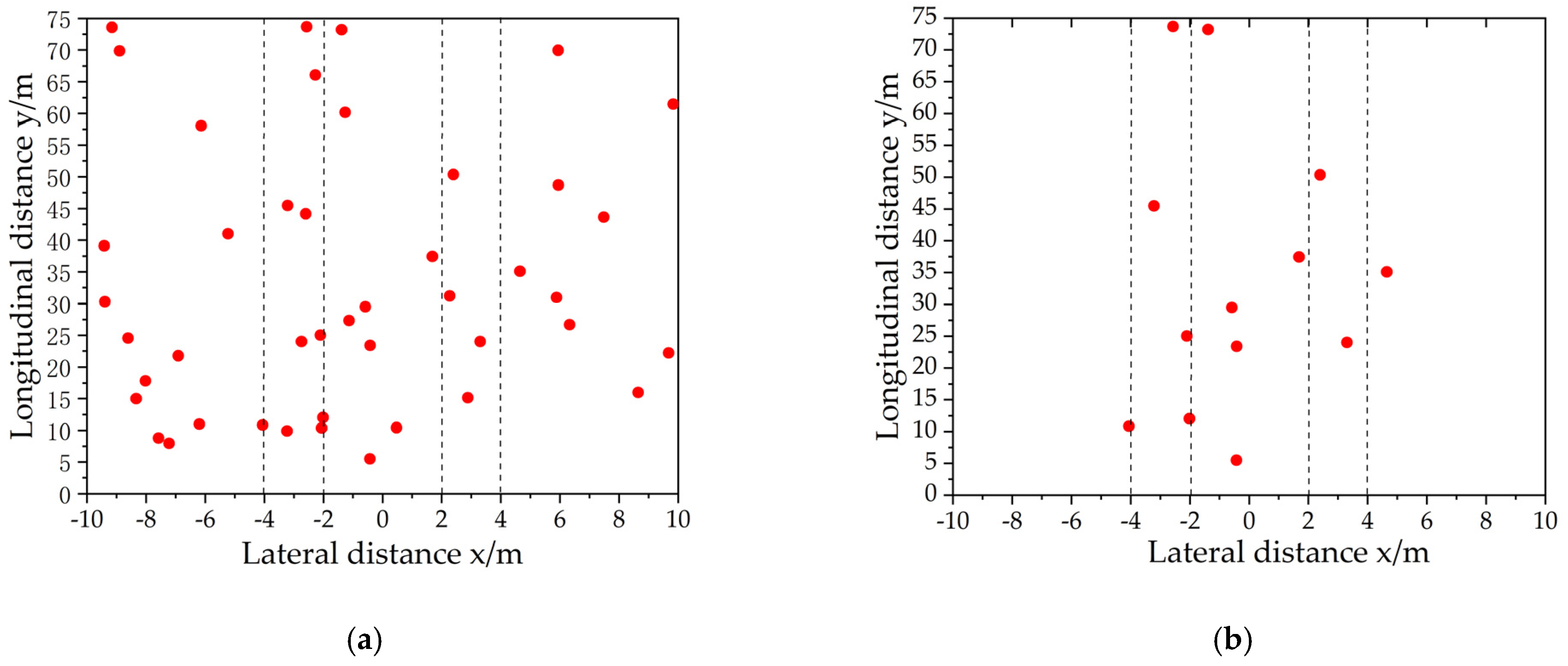
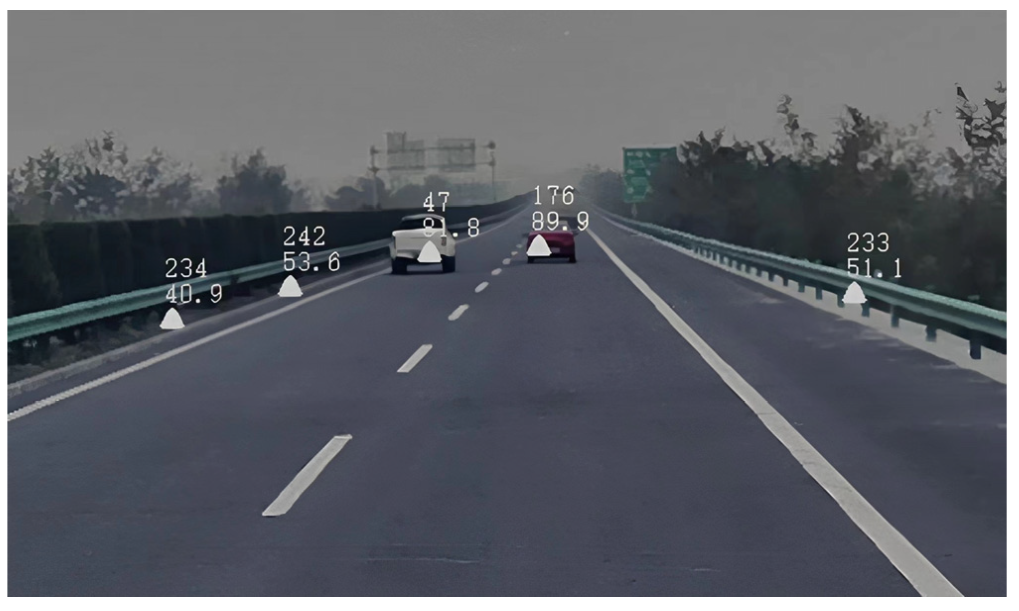
4.2.1. Formation of Regions of Interest
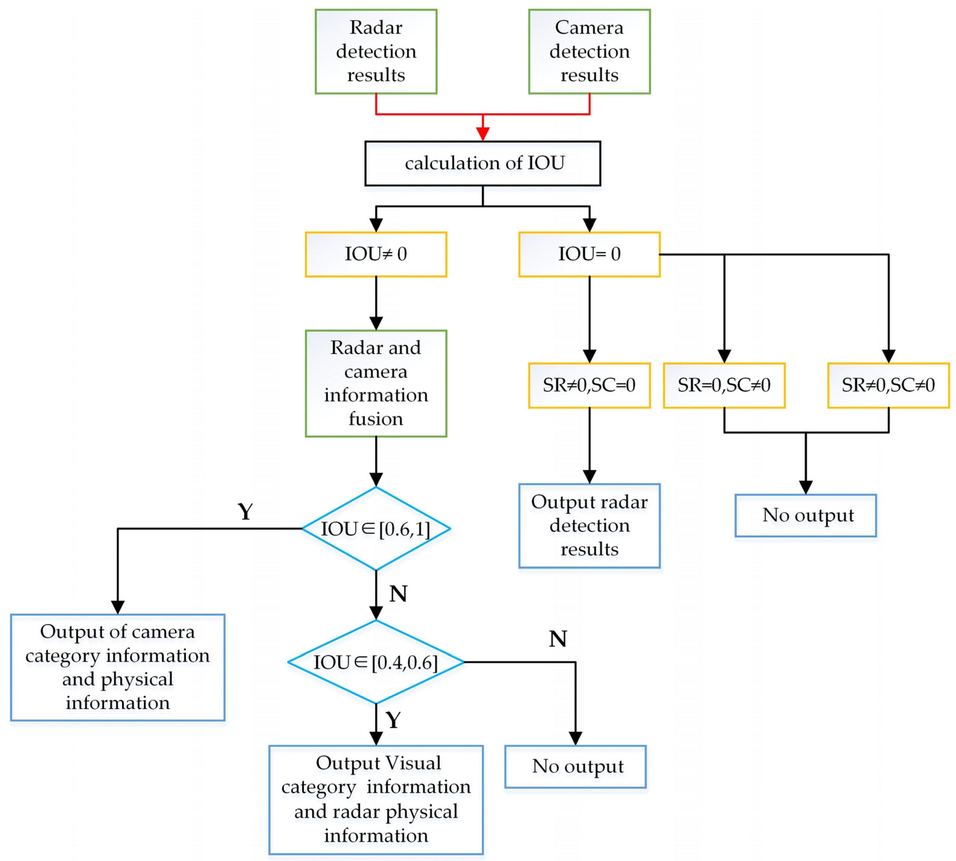
4.2.2. Information Fusion Based on IoU
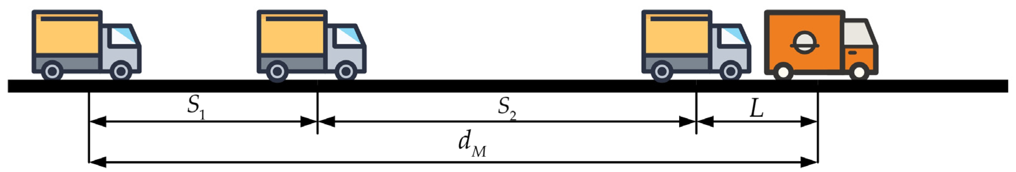
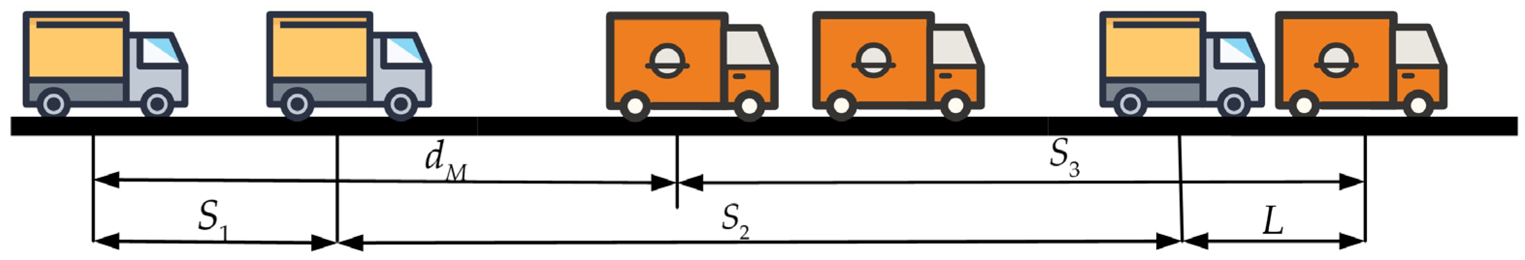
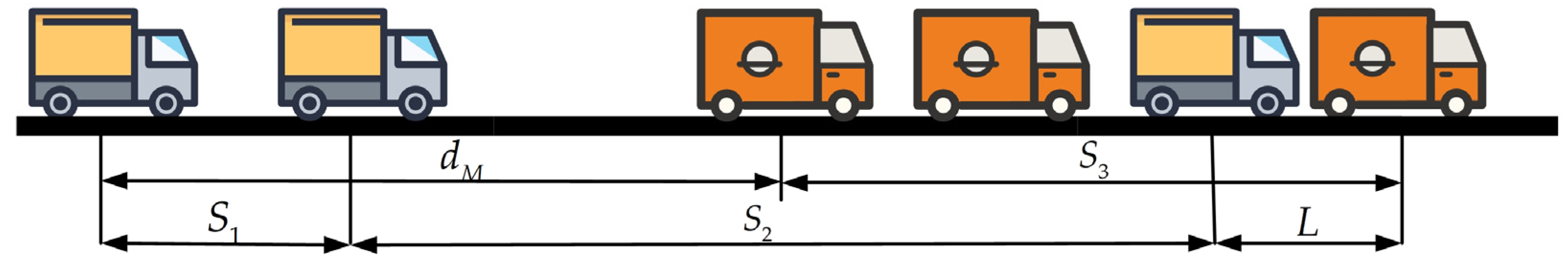
4.3. Forward Collision Warning Strategy
- The host vehicle and the preceding vehicle are moving in the same direction on a straight road segment.
- The host vehicle and the preceding vehicle have similar braking capabilities and deceleration rates.
- The driver of the host vehicle has a constant reaction time and follows a constant headway policy.
- The driver of the preceding vehicle applies a constant deceleration when braking.
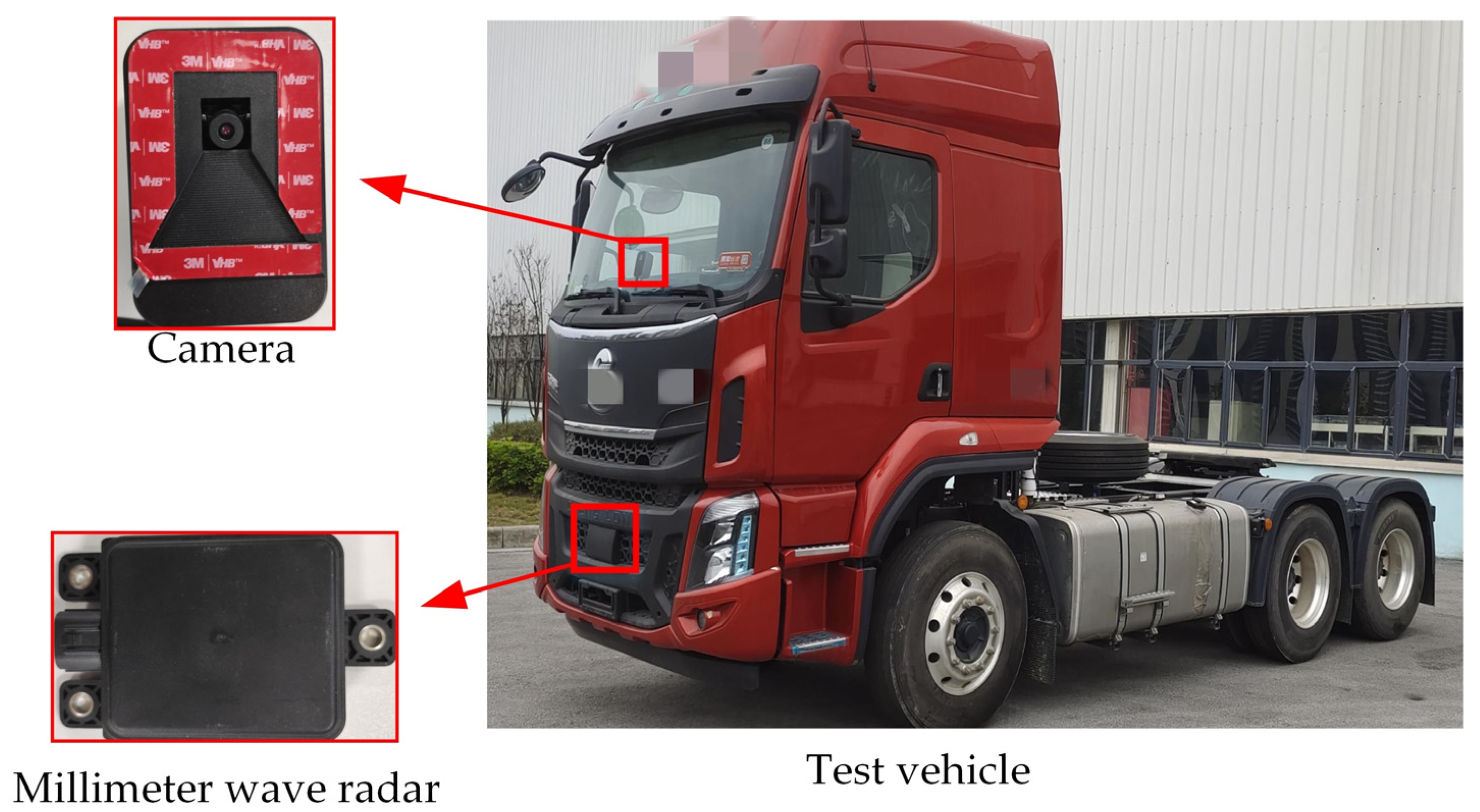
5. Experimental
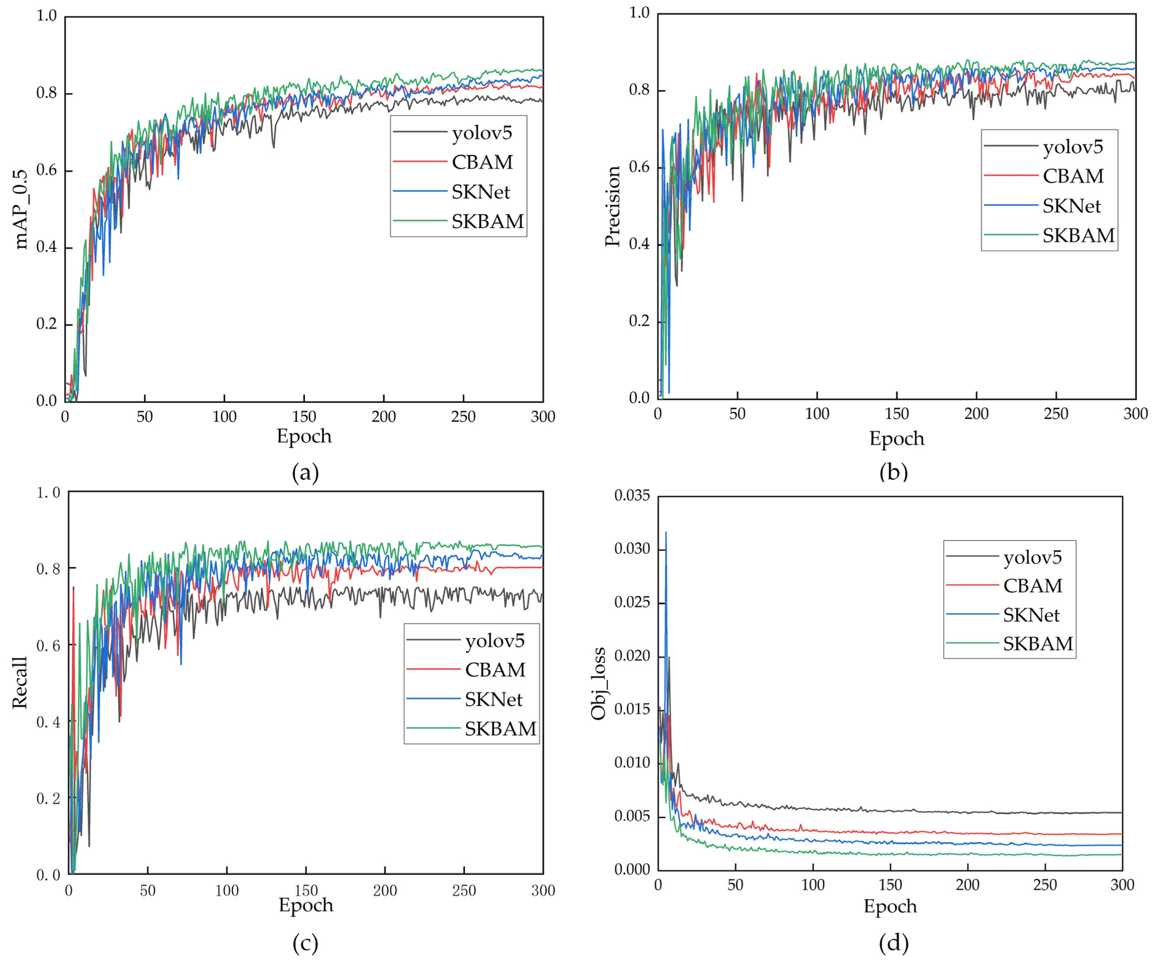
5.1. Improved YOLOv5 Experiment
5.1.1. Vehicle Datasets for Visual Detection
5.1.2. Experimental Environment and Parameter Configuration
5.1.3. Results and Discussion
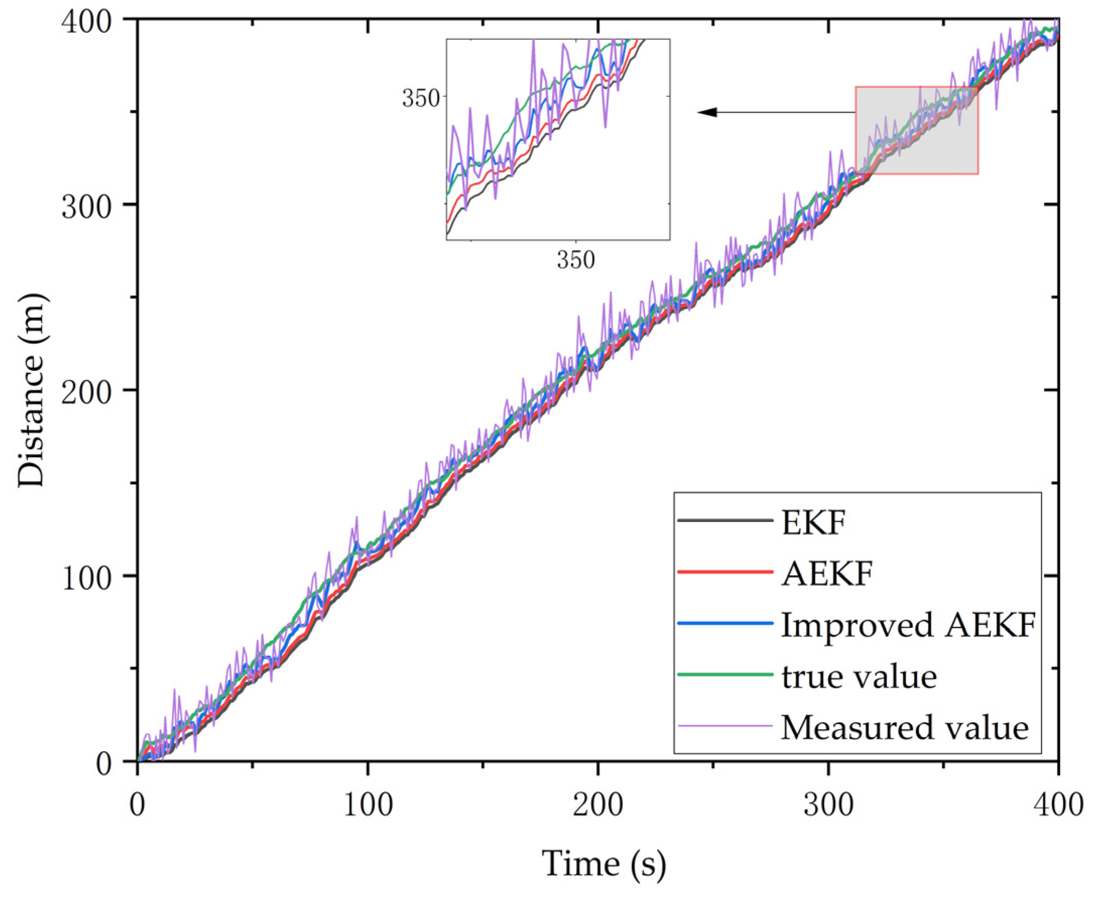
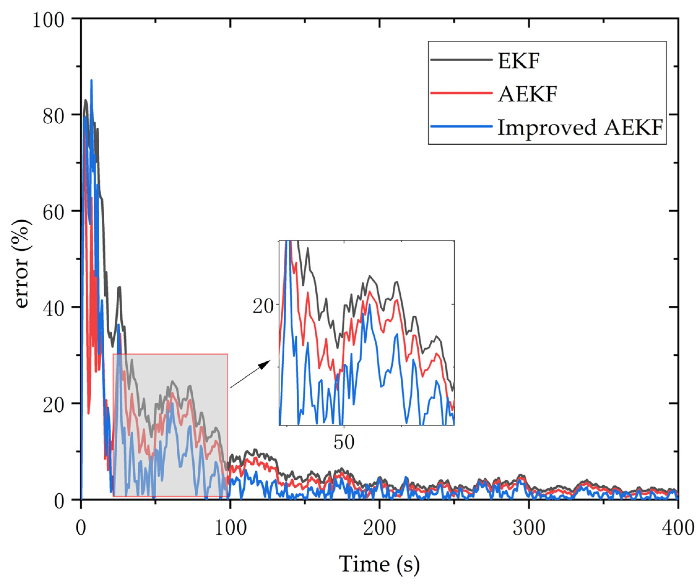
5.2. Improved AEKF Experiment
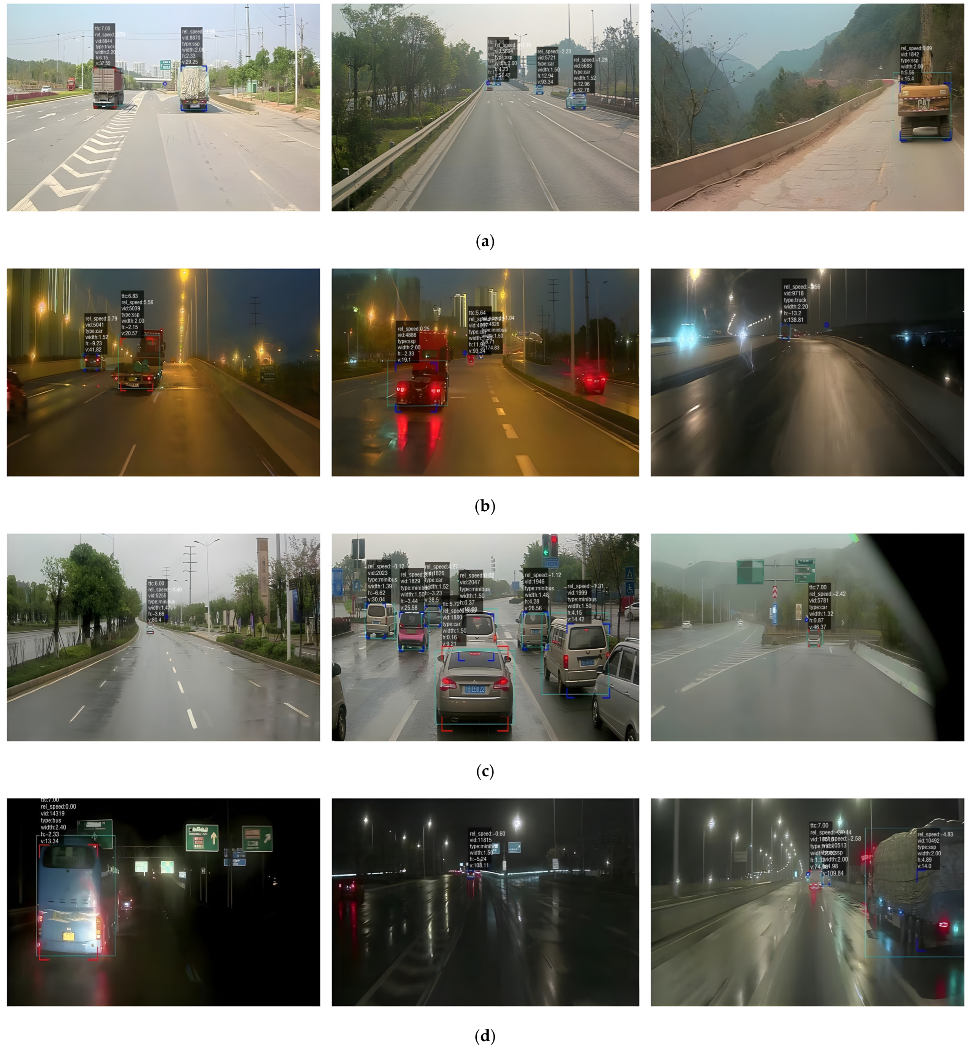
5.3. Collision Warning Experiment
6. Conclusions
Author Contributions
Funding
Institutional Review Board Statement
Informed Consent Statement
Data Availability Statement
Acknowledgments
Conflicts of Interest
References
- Ma, J.; Ding, Y.; Cheng, J.C.P.; Tan, Y.; Gan, V.J.L.; Zhang, J. Analyzing the Leading Causes of Traffic Fatalities Using XGBoost and Grid-Based Analysis: A City Management Perspective. IEEE Access 2019, 7, 148059–148072. [Google Scholar] [CrossRef]
- Lacatan, L.L.; Santos, R.S.; Pinkihan, J.W.; Vicente, R.Y.; Tamargo, R.S. Brake-Vision: A Machine Vision-Based Inference Approach of Vehicle Braking Detection for Collision Warning Oriented System. In Proceedings of the 2021 International Conference on Computational Intelligence and Knowledge Economy (ICCIKE), Dubai, United Arab Emirates, 17–18 March 2021; IEEE: New York, NY, USA, 2021; pp. 485–488. [Google Scholar]
- Ma, X.; Yu, Q.; Liu, J. Modeling Urban Freeway Rear-End Collision Risk Using Machine Learning Algorithms. Sustainability 2022, 14, 12047. [Google Scholar] [CrossRef]
- Baek, M.; Jeong, D.; Choi, D.; Lee, S. Vehicle Trajectory Prediction and Collision Warning via Fusion of Multisensors and Wireless Vehicular Communications. Sensors 2020, 20, 288. [Google Scholar] [CrossRef] [PubMed]
- Jekal, S.; Kim, J.; Kim, D.-H.; Noh, J.; Kim, M.-J.; Kim, H.-Y.; Kim, M.-S.; Oh, W.-C.; Yoon, C.-M. Synthesis of LiDAR-Detectable True Black Core/Shell Nanomaterial and Its Practical Use in LiDAR Applications. Nanomaterials 2022, 12, 3689. [Google Scholar] [CrossRef]
- Li, L.; Zhang, R.; Chen, L.; Liu, B.; Zhang, L.; Tang, Q.; Ding, C.; Zhang, Z.; Hewitt, A.J. Spray drift evaluation with point clouds data of 3D LiDAR as a potential alternative to the sampling method. Front. Plant Sci. 2022, 13, 939733. [Google Scholar] [CrossRef]
- Yan, C.; Xu, W.; Liu, J. Can you trust autonomous vehicles: Contactless attacks against sensors of self-driving vehicle. Def Con 2016, 24, 109. [Google Scholar]
- Lv, P.; Wang, B.; Cheng, F.; Xue, J. Multi-Objective Association Detection of Farmland Obstacles Based on Information Fusion of Millimeter Wave Radar and Camera. Sensors 2022, 23, 230. [Google Scholar] [CrossRef] [PubMed]
- Massoud, Y. Sensor Fusion for 3D Object Detection for Autonomous Vehicles. Ph.D. Thesis, Université d’Ottawa/University of Ottawa, Ottawa, ON, Canada, 2021. [Google Scholar]
- Zhu, Y.; Sun, G.; Ding, G.; Zhou, J.; Wen, M.; Jin, S.; Zhao, Q.; Colmer, J.; Ding, Y.; Ober, E.S. Large-scale field phenotyping using backpack LiDAR and CropQuant-3D to measure structural variation in wheat. Plant Physiol. 2021, 187, 716–738. [Google Scholar] [CrossRef]
- Cui, G.; He, H.; Zhou, Q.; Jiang, J.; Li, S. Research on Camera-Based Target Detection Enhancement Method in Complex Environment. In Proceedings of the 2022 5th International Conference on Robotics, Control and Automation Engineering (RCAE), Changchun, China, 28–30 October 2022; IEEE: New York, NY, USA, 2022; pp. 314–320. [Google Scholar]
- LeCun, Y.; Bengio, Y.; Hinton, G. Deep learning. Nature 2015, 521, 436–444. [Google Scholar] [CrossRef]
- Ren, S.; He, K.; Girshick, R.; Sun, J. Faster r-cnn: Towards real-time object detection with region proposal networks. In Proceedings of the 28th International Conference on Neural Information Processing Systems, Montreal, QC, Canada, 7–12 December 2015. [Google Scholar]
- Girshick, R.; Donahue, J.; Darrell, T.; Malik, J. Rich feature hierarchies for accurate object detection and semantic segmentation. In Proceedings of the IEEE Conference on Computer Vision and Pattern Recognition, Columbus, OH, USA, 23–28 June 2014; pp. 580–587. [Google Scholar]
- He, K.; Zhang, X.; Ren, S.; Sun, J. Spatial pyramid pooling in deep convolutional networks for visual recognition. IEEE Trans. Pattern Anal. Mach. Intell. 2015, 37, 1904–1916. [Google Scholar] [CrossRef]
- Girshick, R. Fast r-cnn. In Proceedings of the IEEE International Conference on Computer Vision, Santiago, Chile, 7–13 December 2015; pp. 1440–1448. [Google Scholar]
- Redmon, J.; Divvala, S.; Girshick, R.; Farhadi, A. You only look once: Unified, real-time object detection. In Proceedings of the IEEE Conference on Computer Vision and Pattern Recognition, Las Vegas, NV, USA, 27–30 June 2016; pp. 779–788. [Google Scholar]
- Liu, W.; Anguelov, D.; Erhan, D.; Szegedy, C.; Reed, S.; Fu, C.; Berg, A.C. Ssd: Single shot multibox detector. In Computer Vision–ECCV 2016, Proceedings of the 14th European Conference, Amsterdam, The Netherlands, 11–14 October 2016; Proceedings; Part I; Springer: Cham, Switzerland, 2016; pp. 21–37. [Google Scholar]
- Zhang, Y.; Guo, Z.; Wu, J.; Tian, Y.; Tang, H.; Guo, X. Real-Time Vehicle Detection Based on Improved YOLO v5. Sustainability 2022, 14, 12274. [Google Scholar] [CrossRef]
- Zheng, H.; Liu, J.; Ren, X. Dim Target Detection Method Based on Deep Learning in Complex Traffic Environment. J. Grid Comput. 2022, 20, 8. [Google Scholar] [CrossRef]
- Lin, Y.; Hu, W.; Zheng, Z.; Xiong, J. Citrus Identification and Counting Algorithm Based on Improved YOLOv5s and DeepSort. Agronomy 2023, 13, 1674. [Google Scholar] [CrossRef]
- Ma, X.; Zhao, R.; Liu, X.; Kuang, H.; Al-qaness, M.A.A. Classification of human motions using micro-Doppler radar in the environments with micro-motion interference. Sensors 2019, 19, 2598. [Google Scholar] [CrossRef] [PubMed]
- Montañez, O.J.; Suarez, M.J.; Fernandez, E.A. Application of Data Sensor Fusion Using Extended Kalman Filter Algorithm for Identification and Tracking of Moving Targets from LiDAR—Radar Data. Remote Sens. 2023, 15, 3396. [Google Scholar] [CrossRef]
- Pearson, J.B.; Stear, E.B. Kalman filter applications in airborne radar tracking. IEEE Trans. Aerosp. Electron. Syst. 1974, 3, 319–329. [Google Scholar] [CrossRef]
- Liu, T.; Du, S.; Liang, C.; Zhang, B.; Feng, R. A novel multi-sensor fusion based object detection and recognition algorithm for intelligent assisted driving. IEEE Access 2021, 9, 81564–81574. [Google Scholar] [CrossRef]
- Jiang, C.; Wang, Z.; Liang, H. Target detection and adaptive tracking based on multisensor data fusion in a smoke environment. In Proceedings of the 2022 8th International Conference on Control, Automation and Robotics (ICCAR), Xiamen, China, 8–10 April 2022; IEEE: New York, NY, USA, 2022; pp. 420–425. [Google Scholar]
- Zhou, Y.; Dong, Y.; Hou, F.; Wu, J. Review on Millimeter-Wave Radar and Camera Fusion Technology. Sustainability 2022, 14, 5114. [Google Scholar] [CrossRef]
- Lin, J.-J.; Guo, J.-I.; Shivanna, V.M.; Chang, S.-Y. Deep Learning Derived Object Detection and Tracking Technology Based on Sensor Fusion of Millimeter-Wave Radar/Video and Its Application on Embedded Systems. Sensors 2023, 23, 2746. [Google Scholar] [CrossRef]
- Dong, J.; Chu, L. Coupling Safety Distance Model for Vehicle Active Collision Avoidance System; SAE International: Warrendale, PA, USA, 2019. [Google Scholar]
- Alsuwian, T.; Saeed, R.B.; Amin, A.A. Autonomous Vehicle with Emergency Braking Algorithm Based on Multi-Sensor Fusion and Super Twisting Speed Controller. Appl. Sci. 2022, 12, 8458. [Google Scholar] [CrossRef]
- Liu, G.; Wang, L. A Safety Distance Automatic Control Algorithm for Intelligent Driver Assistance System; Springer International Publishing: Cham, Switzerland, 2021; pp. 645–652. [Google Scholar]
- Lin, H.-Y.; Dai, J.-M.; Wu, L.-T.; Chen, L.-Q. A Vision-Based Driver Assistance System with Forward Collision and Overtaking Detection. Sensors 2020, 20, 5139. [Google Scholar] [CrossRef]
- Wong, M.K.; Connie, T.; Goh, M.K.O.; Wong, L.P.; Teh, P.S.; Choo, A.L. A visual approach towards forward collision warning for autonomous vehicles on Malaysian public roads. F1000Research 2021, 10, 928. [Google Scholar] [CrossRef]
- Pak, J.M. Hybrid Interacting Multiple Model Filtering for Improving the Reliability of Radar-Based Forward Collision Warning Systems. Sensors 2022, 22, 875. [Google Scholar] [CrossRef]
- Wei, Z.; Zhang, F.; Chang, S.; Liu, Y.; Wu, H.; Feng, Z. Mmwave radar and vision fusion for object detection in autonomous driving: A review. Sensors 2022, 22, 2542. [Google Scholar] [CrossRef] [PubMed]
- Yu, M.; Wan, Q.; Tian, S.; Hou, Y.; Wang, Y.; Zhao, J. Equipment Identification and Localization Method Based on Improved YOLOv5s Model for Production Line. Sensors 2022, 22, 10011. [Google Scholar] [CrossRef] [PubMed]
- Li, Z.; Song, J.; Qiao, K.; Li, C.; Zhang, Y.; Li, Z. Research on efficient feature extraction: Improving YOLOv5 backbone for facial expression detection in live streaming scenes. Front. Comput. Neurosci. 2022, 16, 980063. [Google Scholar] [CrossRef] [PubMed]
- Zhu, X.; Lyu, S.; Wang, X.; Zhao, Q. TPH-YOLOv5: Improved YOLOv5 based on transformer prediction head for object detection on drone-captured scenarios. In Proceedings of the 2021 IEEE/CVF International Conference on Computer Vision Workshops (ICCVW), Montreal, BC, Canada, 11–17 October 2021; pp. 2778–2788. [Google Scholar]
- Hu, J.; Shen, L.; Sun, G. Squeeze-and-excitation networks. In Proceedings of the IEEE Conference on Computer Vision and Pattern Recognition, Salt Lake City, UT, USA, 18–23 June 2018; pp. 7132–7141. [Google Scholar]
- Zhu, X.; Cheng, D.; Zhang, Z.; Lin, S.; Dai, J. An empirical study of spatial attention mechanisms in deep networks. In Proceedings of the IEEE/CVF International Conference on Computer Vision, Seoul, Republic of Korea, 27 October–2 November 2019; pp. 6688–6697. [Google Scholar]
- Hou, Q.; Zhou, D.; Feng, J. Coordinate attention for efficient mobile network design. In Proceedings of the IEEE/CVF Conference on Computer Vision and Pattern Recognition, Nashville, TN, USA, 20–25 June 2021; pp. 13713–13722. [Google Scholar]
- Woo, S.; Park, J.; Lee, J.; Kweon, I.S. Cbam: Convolutional block attention module. In Proceedings of the European Conference on Computer Vision (ECCV), Munich, Germany, 8–14 September 2018; pp. 3–19. [Google Scholar]
- Li, X.; Wang, W.; Hu, X.; Yang, J. Selective kernel networks. In Proceedings of the IEEE/CVF Conference on Computer Vision and Pattern Recognition, Long Beach, CA, USA, 15–20 June 2019; pp. 510–519. [Google Scholar]
- Park, J.; Woo, S.; Lee, J.; Kweon, I.S. Bam: Bottleneck attention module. arXiv 2018, arXiv:1807.06514. [Google Scholar]
- Akhlaghi, S.; Zhou, N. Adaptive multi-step prediction based EKF to power system dynamic state estimation. In Proceedings of the 2017 IEEE Power and Energy Conference at Illinois (PECI), Champaign, IL, USA, 23–24 February 2017; IEEE: New York, NY, USA, 2017; pp. 1–8. [Google Scholar]
- Tian, Y.; Lai, R.; Li, X.; Xiang, L.; Tian, J. A combined method for state-of-charge estimation for lithium-ion batteries using a long short-term memory network and an adaptive cubature Kalman filter. Appl. Energy 2020, 265, 114789. [Google Scholar] [CrossRef]
- Wang, J. Stochastic Modeling for Real-Time Kinematic GPS/GLONASS Positioning. Navigation 1999, 46, 297–305. [Google Scholar] [CrossRef]
- Lundagårds, M. Vehicle Detection in Monochrome Images; Institutionen för Systemteknik: Linköping, Sweden, 2008. [Google Scholar]
- Rezatofighi, H.; Tsoi, N.; Gwak, J.; Sadeghian, A.; Reid, I.; Savarese, S. Generalized intersection over union: A metric and a loss for bounding box regression. In Proceedings of the IEEE/CVF Conference on Computer Vision and Pattern Recognition, Long Beach, CA, USA, 15–20 June 2019; pp. 658–666. [Google Scholar]
- Yang, L.; Luo, P.; Change Loy, C.; Tang, X. A large-scale car dataset for fine-grained categorization and verification. In Proceedings of the IEEE Conference on Computer Vision and Pattern Recognition, Boston, MA, USA, 7–12 June 2015; pp. 3973–3981. [Google Scholar]
- Wen, L.; Du, D.; Cai, Z.; Lei, Z.; Chang, M.; Qi, H.; Lim, J.; Yang, M.; Lyu, S. UA-DETRAC: A new benchmark and protocol for multi-object detection and tracking. Comput. Vis. Image Underst. 2020, 193, 102907. [Google Scholar] [CrossRef]
- Akhlaghi, S.; Zhou, N.; Huang, Z. Adaptive adjustment of noise covariance in Kalman filter for dynamic state estimation. In Proceedings of the 2017 IEEE Power & Energy Society General Meeting, Chicago, IL, USA, 16–20 July 2017; IEEE: New York, NY, USA, 2017; pp. 1–5. [Google Scholar]


| Name | Precision (%) | mAP (%) | Recall (%) | FPS |
|---|---|---|---|---|
| YOLOv5 | 80.01 | 78.27 | 73.17 | 82 |
| YOLOv5 + CBAM | 83.27 | 82.11 | 80.09 | 63 |
| YOLOv5 + SKNet | 85.90 | 84.71 | 83.37 | 73 |
| YOLOv5 + SKBAM | 87.36 | 86.19 | 85.34 | 67 |
| Day or Night Environment | Sunny or Rainy | Algorithm | Alarms (Times) | Missed Alarms (Times) | False Alarms (Times) | Accuracy (%) | Missed Alarm Rate (%) | False Alarm Rate (%) |
|---|---|---|---|---|---|---|---|---|
| Day | Sunny | Tradition | 937 | 13 | 23 | 96.211 | 1.387 | 2.455 |
| Ours | 926 | 8 | 17 | 97.323 | 0.864 | 1.836 | ||
| rainy | Tradition | 2376 | 83 | 156 | 90.281 | 3.493 | 6.566 | |
| Ours | 2039 | 67 | 121 | 91.073 | 3.286 | 5.934 | ||
| Night | Sunny | Tradition | 763 | 39 | 10 | 93.890 | 5.111 | 1.311 |
| Ours | 973 | 33 | 13 | 95.427 | 3.392 | 1.336 | ||
| rainy | Tradition | 386 | 31 | 8 | 90.647 | 8.031 | 2.073 | |
| Ours | 393 | 27 | 18 | 89.286 | 6.870 | 4.580 | ||
| aggregate | Tradition | 4462 | 166 | 197 | 92.156 | 3.720 | 4.415 | |
| Ours | 4331 | 135 | 169 | 93.193 | 3.117 | 3.902 | ||
Disclaimer/Publisher’s Note: The statements, opinions and data contained in all publications are solely those of the individual author(s) and contributor(s) and not of MDPI and/or the editor(s). MDPI and/or the editor(s) disclaim responsibility for any injury to people or property resulting from any ideas, methods, instructions or products referred to in the content. |
© 2023 by the authors. Licensee MDPI, Basel, Switzerland. This article is an open access article distributed under the terms and conditions of the Creative Commons Attribution (CC BY) license (https://creativecommons.org/licenses/by/4.0/).
Share and Cite
Sun, C.; Li, Y.; Li, H.; Xu, E.; Li, Y.; Li, W. Forward Collision Warning Strategy Based on Millimeter-Wave Radar and Visual Fusion. Sensors 2023, 23, 9295. https://doi.org/10.3390/s23239295
Sun C, Li Y, Li H, Xu E, Li Y, Li W. Forward Collision Warning Strategy Based on Millimeter-Wave Radar and Visual Fusion. Sensors. 2023; 23(23):9295. https://doi.org/10.3390/s23239295
Chicago/Turabian StyleSun, Chenxu, Yongtao Li, Hanyan Li, Enyong Xu, Yufang Li, and Wei Li. 2023. "Forward Collision Warning Strategy Based on Millimeter-Wave Radar and Visual Fusion" Sensors 23, no. 23: 9295. https://doi.org/10.3390/s23239295
APA StyleSun, C., Li, Y., Li, H., Xu, E., Li, Y., & Li, W. (2023). Forward Collision Warning Strategy Based on Millimeter-Wave Radar and Visual Fusion. Sensors, 23(23), 9295. https://doi.org/10.3390/s23239295