Damage Identification in Cement-Based Structures: A Method Based on Modal Curvatures and Continuous Wavelet Transform

Abstract

Modal analysis is an effective tool in the context of Structural Health Monitoring (SHM) since the dynamic characteristics of cement-based structures reflect the structural health status of the material itself. The authors consider increasing level load tests on concrete beams and propose a methodology for damage identification relying on the computation of modal curvatures combined with continuous wavelet transform (CWT) to highlight damage-related changes. Unlike most literature studies, in the present work, no numerical models of the undamaged structure were exploited. Moreover, the authors defined synthetic damage indices depicting the status of a structure. The results show that the I mode shape is the most sensitive to damages; indeed, considering this mode, damages cause a decrease of natural vibration frequency (up to approximately −67%), an increase of loss factor (up to approximately fivefold), and changes in the mode shapes morphology (a cuspid appears). The proposed damage indices are promising, even if the level of damage is not clearly distinguishable, probably because tests were performed after the load removal. Further investigations are needed to scale the methodology to in-field applications.

1. Introduction

Structural Health Monitoring (SHM) technologies are pivotal for the management of cement-based structures and infrastructures, which can be frequently subjected to destructive factors causing damage to the structure itself. Indeed, both the costs and life cycle of structures and infrastructures can be optimized through the regular monitoring of relevant parameters, providing a broad picture of the health status of the supervised structure, and avoiding rapid damage propagation. Given the relevant costs of inspection, maintenance, and intervention operations, the SHM techniques can play an essential role in assessing damages or even predicting their occurrence. The advantages concerning inspections are unquestionable, given the prompt identification of structural issues and the consequent planning of deeper inspection operations, providing an invaluable contribution, especially for critical structures [1]. Moreover, monitoring tools also allow for the inclusion of environmental parameters in the evaluation, properly considering their effect on the measured signals, varying with these factors [2,3]. In this regard, Ietka et al. [4] highlighted the correlation between temperature and displacement in a bridge case study. However, even with all the potentialities of SHM strategies, at present, it is not easy to widely diffuse the installation of a SHM system on buildings or infrastructures, since the potential economic benefit is not so straightforward to final users [5,6], despite the possibility of achieving completely automated monitoring systems through the exploitation of sophisticated smart sensors and also Artificial Intelligence (AI) tools [7,8].

In the last decades, several different technologies have been exploited to this aim, each showing pros and cons; among them, it is worthy to cite self-sensing/monitoring techniques (where electrical impedance sensors are strictly related to materials with conductive additions enhancing their self-sensing/monitoring capability [9]) and smart sensor networks exploiting deep learning computing tools [1], acoustic sensors [10], piezoelectric transducers [11], non-contact vibration sensors [12], accelerometers [13], etc. Different time scales can be considered for diagnosis, also in (near) real-time, hence useful for emergency operations [14] and also in combination with early warning systems [15,16]. Sometimes static analyses have been exploited, for example with parameter identification to identify damages in frame structures [17] or stiffness separation method on truss structures [18]. Vibrational analysis (in particular, operational modal analysis coupled with proper signal processing techniques [19]) can depict the dynamical performance of a structure and reflects eventual changes due to disrupting events [20] (e.g., earthquakes [21]) or deterioration processes (e.g., contaminants penetration). In fact, in case of damage, the dynamic response of the structure is different with respect to the undamaged status [22]. Mass, stiffness, and damping values are altered, reflecting in changes in terms of modal parameters (i.e., natural frequency and loss factor) as well as of mode shapes and related modal curvatures [23,24,25] (also known as rotational modes [26]), which are the second derivative of mode shapes, usually computed according to the central difference approximation method [22]. Sometimes, the flexibility matrix has also been considered for damage identification purposes, being more effective at low frequency with respect to the stiffness matrix [25]. Modal curvatures are generally more affected by singularities concerning the corresponding mode shapes; in fact, the curvature is related to the structure stiffness, which in turn varies with the presence of cracks (i.e., local damages [27]). Therefore, the local stiffness reduction due to the formation of a crack makes the curvature lose continuity [28]. Impact tests have been extensively exploited in the literature for damage identification in concrete structures [29]; however, a significant number of issues can occur in experimental conditions, making it difficult to estimate the second derivative of mode shapes with high accuracy [30], especially in noisy environments, where dedicated processing techniques are needed [31]. Moreover, while on concrete plain structures, the damage can be considered as a concentrated defect, in reinforced concrete elements the intrinsic heterogeneity leads to non-linear behaviours, which cause diffuse cracking phenomena, possibly masking the effect of singularities. This behaviour is also enhanced by the quasi-static nature of the applied loads (e.g., monotonic or cycling loading). A common approach to analyze this type of damage is the evaluation of the natural frequency reduction, which appears very evident in the initial cracking phase (up to 25–55% in the yield state [32,33]). Its measurement appears quite straightforward, hence this method can be widely exploited for damage localization [34]. Moreover, adding virtual mass to a structure can be effective in the enhancement of sensitivity toward damages [35]. On the other hand, damping ratios are challenging to measure, being not so regular [36] and consequently not commonly exploited for damage identification.

Several studies consider numerical models to discuss the relationship between the presence of damages and the related changes in modal parameters. In fact, since the information related to the intact structure is frequently unavailable and many approaches are based on a comparison with this time, numerical models can fill this gap. However, there are inevitable simplifications in the modelling procedures, not suffering from noise and disturbing sources, differently from experimental cases. Indeed, to effectively deal with noisy data typical of experimental campaigns, different routes can be pursued [28]: (i) design an optimal sampling in order to reduce errors when computing modal curvatures [37]; (ii) exploit suitable filtering techniques (e.g., Laplacian scheme [38] or Teager energy operator and wavelets [39]); (iii) use effective post processing techniques (e.g., fuzzy logic [40,41]).

Moreover, many studies in the literature define damage-related indices to investigate the structural health status of a structure concisely. Meruane et al. [42] developed a mathematical framework for damage detection in steel-concrete composites subjected to impact tests: they studied the changes in stiffness due to damage occurrence and evaluated the correlation with the initial condition through the modal assurance criterion (MAC). A damage index based on curvatures (i.e., the absolute difference in curvature between damaged and intact structures) was synthesized to depict the distribution of damages. In fact, sharp changes in modal curvatures are caused by structural damage. Indeed, the absolute difference in terms of modal curvatures between damaged and undamaged states is quite widely exploited in the literature [43]; Pranno et al. [22] defined a Curvature Damage Factor (CDF), averaging the differences in modal curvatures considering a certain number of mode shapes in damaged/undamaged configurations; also in this case, a simulation-based damage detection approach was proposed to evaluate the stiffness degradation with progressive damage occurrence. They also underlined the relevance of the inverse eigenvalue sensitivity method [44] for identifying damages through variations in terms of natural vibration frequencies. Jahangir et al. [45] proposed different damage indices based on single, double, and triple damage scenarios represented in a numerical model; they calculated the energy associated with the wavelet coefficients through the Shannon entropy and defined two indices able to localize the damage and assess its severity. Indeed, wavelets have been demonstrated to be sensitive to the presence of damages (e.g., Haar and Gabor wavelets for crack detection [46]) and represent a powerful tool to be exploited in this context, along with numerical methods. Masciotta and Pellegrini [47] proposed an index based on the imaginary component of mode shapes in different damage conditions; in particular, they considered the difference in the imaginary part (normalized with respect to the initial average imaginary content) and multiplied it by the ratio between natural frequency in damaged and undamaged conditions, evidencing the higher sensitivity to damage occurrence with respect to the real component. Bayissa et al. [48] exploited continuous wavelet transform (CWT) to derive the energy distribution in the time-frequency domain and transform the wavelet coefficients into damage identification parameters.

Some studies investigated also the damage severity, which can be related to the energy of wavelet coefficients computed in correspondence with the diverse degrees of freedom (DOFs) [45]. Moreover, Jahangir et al. [49] evidenced that wavelets are efficient in eliminating noise that could contaminate curvatures and prevent correct damage detection through singularity identification. Starting from the details signal provided by the wavelet analysis, they also proposed a normalized damage index to be computed for each DOF, to localize the damage according to a specific threshold. The use of wavelets can be necessary to highlight discontinuities also in the presence of relatively small damages, which could be easily masked by noise; however, wavelets also inherit global fluctuations, therefore sometimes they are not sufficient. In those cases, the Teager energy operator can be exploited to intensify local singularities while removing global trend fluctuations; Sha et al. [50] exploited this approach and proposed a damage index based on data fusion of multiple mode shapes analysed through wavelets and Teager energy operator techniques.

Also, the variability of modal parameters must be considered; indeed, both environmental and material-intrinsic factors can make natural vibration frequency change and this needs to be distinguished from variations caused by a damage occurrence. Anastasopoulos et al. [51] found the same sensitivity of natural frequency towards damage and temperature; Maes et al. [52] proposed to use of the Principal Component Analysis (PCA) to remove the variations due to natural factors when validating vibration-based SHM on a retrofitted railway bridge. In general, repeatability tests should be performed to evaluate the robustness of a specific method.

The information deriving from a modal analysis could also represent an added value to be exploited in AI-based techniques for SHM [53,54]. Indeed, SHM-related data processing can provide multi-domain information supporting decision-making strategies [55] and really making a difference, even more through the exploitation of machine learning (ML) algorithms, especially the unsupervised ones, not requiring fully labelled data [55], or deep learning approaches [56]. However, for this aim great amounts of data are needed for proper model training and this goes beyond the scope of this work.

This manuscript aims at:

• Evaluating the changes in terms of modal parameters of scaled concrete beams subjected to loading tests leading to cracking phenomena.
• Analyzing the modal curvatures also through continuous wavelet transform.
• Proposing damage indices considering both the curvature change and the CWT-based analysis.
• Evaluating the sensitivity of the results with respect to data processing parameters.

Scaled concrete beams were manufactured with a self-sensing mix design; loading tests were performed at different levels by using a mechanical press. After each loading phase, an impact test was performed to assess the dynamic behaviour of the concrete elements. Modal analysis was conducted, and modal curvatures were analyzed, also exploiting CWT. Finally, different damage indices were proposed.

The paper is organised as follows: Section 2 describes the materials and methods employed in the study, starting with the description of the concrete specimens and their mix design and the load tests performed. Then, the techniques adopted for modal analysis and modal curvature computation are reported, together with the definition of damage-related indices. Hence, the methods for sensitivity analysis towards processing parameters are detailed. The results are reported and discussed in Section 3. Finally, the authors draw the conclusions in Section 4, where also possible future developments are depicted.

2. Materials and Methods

Concrete specimens were manufactured according to the mix design reported in

Table 1. Mix-design of concrete specimens.

Cement [kg/m3]	Water [kg/m3]	Air [%]	Sand [kg/m3]	Intermediate Gravel [kg/m3]	Coarse Gravel [kg/m3]	RCF [kg/m3]	BCH [kg/m3]
470.0	235.0	2.5	795.0	321.0	476.0	0.9	10.0

; the water/cement (w/c) ratio was equal to 0.50 by mass and the workability class was S5 assessed through the slump Abrams cone. It is worth noting that the selection (and dosages) of conductive carbon-based additions, namely recycled carbon fibres (RCF) and biochar (BCH), was made according to the findings of a previous study [9] (furthermore, the developed mix-design and the related measurement system have already been patented—“Eco-compatible and self-sensing mortar and concrete compositions for manufacturing reinforced and non-reinforced constructive elements, related construction element and methods for the realization of self-monitorable building structures”, patent n. 102020000022024); these materials enhance the self-sensing capabilities of cement-based elements, but the related analysis goes beyond the scope of this paper.

A concrete mixer was used for casting and the following steps were accomplished:

-

Mixing of sand and intermediate/coarse gravels (2 min).

-

Addition of cement and further mixing (2 min).

-

Addition of BCH and further mixing (7 min).

-

Addition of RCF and further mixing (2 min).

-

Water addition and further mixing (10 min).

-

Pouring of fresh mix in moulds.

A total of 12 prismatic (10 cm × 10 cm × 50 cm) specimens were cast; they were reinforced with a corrugated stainless-steel rebar placed in the middle. Prismatic specimens were divided as follows:

-

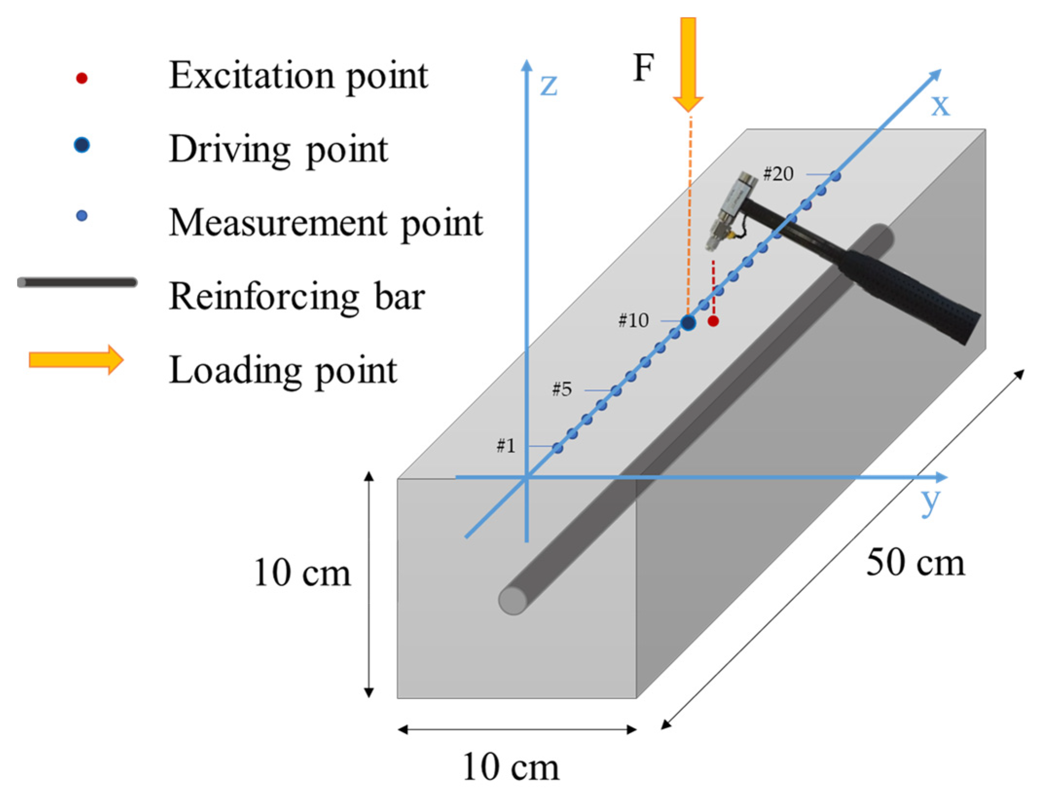
n. 6 sensorized specimens: sensors for the measurement of electrical impedance and free corrosion potential were embedded in the specimens for SHM purposes (both beyond the scope of this article, but very important to continuously monitor the health status of the material). Plastic tubes were employed for easing the cable routing; they require particular attention since they inevitably contribute to the determination of the element dynamic behaviour. The layout of the specimens is reported in Figure 1.

-

n. 6 non-sensorized specimens: these were manufactured to evaluate the effect of the embedded sensors on the dynamic behaviour of the elements (rigidity should be affected by sensors, representing discontinuities in the material) and the consequent modal parameters. Half of them were dedicated to the assessment of flexural strength according to the EN 12390-5 standard [57]; the obtained value was relevant for the design of the loading tests to be performed on the concrete beams.

Figure 1. Layout of the sensorized concrete specimens: (a) Design; (b) Mold for casting phase.

Figure 1. Layout of the sensorized concrete specimens: (a) Design; (b) Mold for casting phase.

After the standard curing period (i.e., 28 days) in environmental conditions, stainless-steel washers were installed with a bicomponent resin to serve as bases for the positioning of accelerometers for the vibrational analysis. Hence, the specimens were subjected to loading tests. Increasing load levels were determined depending on the mechanical resistance preliminarily measured on dedicated specimens.

The loading tests were executed through a mechanical press (Zwick Roell, maximum load: 600 kN, Figure 2). The concrete specimen was positioned on two pins (i.e., pinned conditions) at 30 cm from each other (i.e., 10 cm from the beam ends); the load was applied on the specimen centre, with a velocity of 0.1 mm/min. Three different loads were applied (and the corresponding test times were named as reported hereafter), namely:

• 90% of the fracture load assessed on dedicated specimens (t1).
• Fracture load (i.e., the load at which the first crack forms), specific for the specimen under test (t2).
• The load at which the crack aperture is approximately 1 mm (t3).

The initial time, when the specimen was intact, was called t0.

At t0 and after each load trial, a vibrational analysis was performed; an impact hammer (PCB 086 B04, PCB Piezotronics, Depew, NY, USA) was employed to excite the structure (force given in −z direction, see Figure 3), hence the structural response was measured through accelerometers (measuring on z direction) positioned along the specimen mid-line; 20 DOFs were considered, with an interaxle spacing of 2.5 cm from each other (Figure 3). The DOF #10 can be considered the driving point, given that the energy path from the excitation point is short enough (<5 mm, according to the sensor dimensions).

A total of 5 accelerometers (PCB 352C33, PCB Piezotronics) were employed; hence, 5 simultaneous responses were measured, and then the accelerometers were positioned in the consequent measurement points. Four measurements were performed to cover the whole specimen, as reported in Figure 4. The input force was used as a trigger, to record the transient and the damped dynamical response. Each acquisition lasted 0.25 s; the frequency range considered was 0–4096 Hz, i.e., sampling frequency equal to 8192 Hz and 1024 spectral lines (with a frequency resolution of 4 Hz); 5 repeated acquisitions were performed on each measurement point and the average was computed to increase the Signal-to-Noise Ratio (SNR). The LMS SCADAS Mobile (Siemens, Munich, Germany) was exploited as an acquisition system; the connection configuration is reported in Figure 5.

2.1. Modal Analysis, Modal Curvatures Computation, and Damage Indices Definition

The modal analysis was conducted through the LMS SCADAS Mobile proprietary software, i.e., the Simcenter Testlab Impact testing module. In particular, the acceleration signals were analysed in relation to the force given by the impact hammer (measured through the embedded load cell) to obtain the Frequency Response Functions (FRFs), which in turn allow to compute the modal parameters of the structural element, hence representing an important tool for damage identification [58].

Data processing allows to visualisation of the vibration distribution on the specimen under test, hence it is possible to identify the areas most subjected to vibration or with discontinuities that could be related to the presence of damages (but also to the presence of embedded sensors). Observing the response signal in the time domain, it is possible to notice an amplification of the excitation when the frequency is close to the structure natural frequency (in correspondence with which the amplitude is maximum). Indeed, the FRF behaves like a filter related to the input force: it amplifies the force at the resonance frequency, whereas it decreases it at antiresonance. Modal shapes can be identified for the different resonance frequencies; the complexity of vibrational modes increases with frequency. It is worth underlining that no displacements are present at nodal lines, and this can be detrimental if we want to exploit vibrational analysis to detect damages close to nodal lines.

Mode shapes are derived through experimental modal analysis based on interpolation methods. In particular, the FRF in terms of acceleration, i.e., the Inertance, was considered. The vibration maps are obtained from the FRFs evaluated as estimators in the frequency domain, according to (1):

$$H_1\left(\omega \right)=\frac{S_{fv}\left(\omega \right)}{S_{ff}\left(\omega \right)}$$

(1)

where:

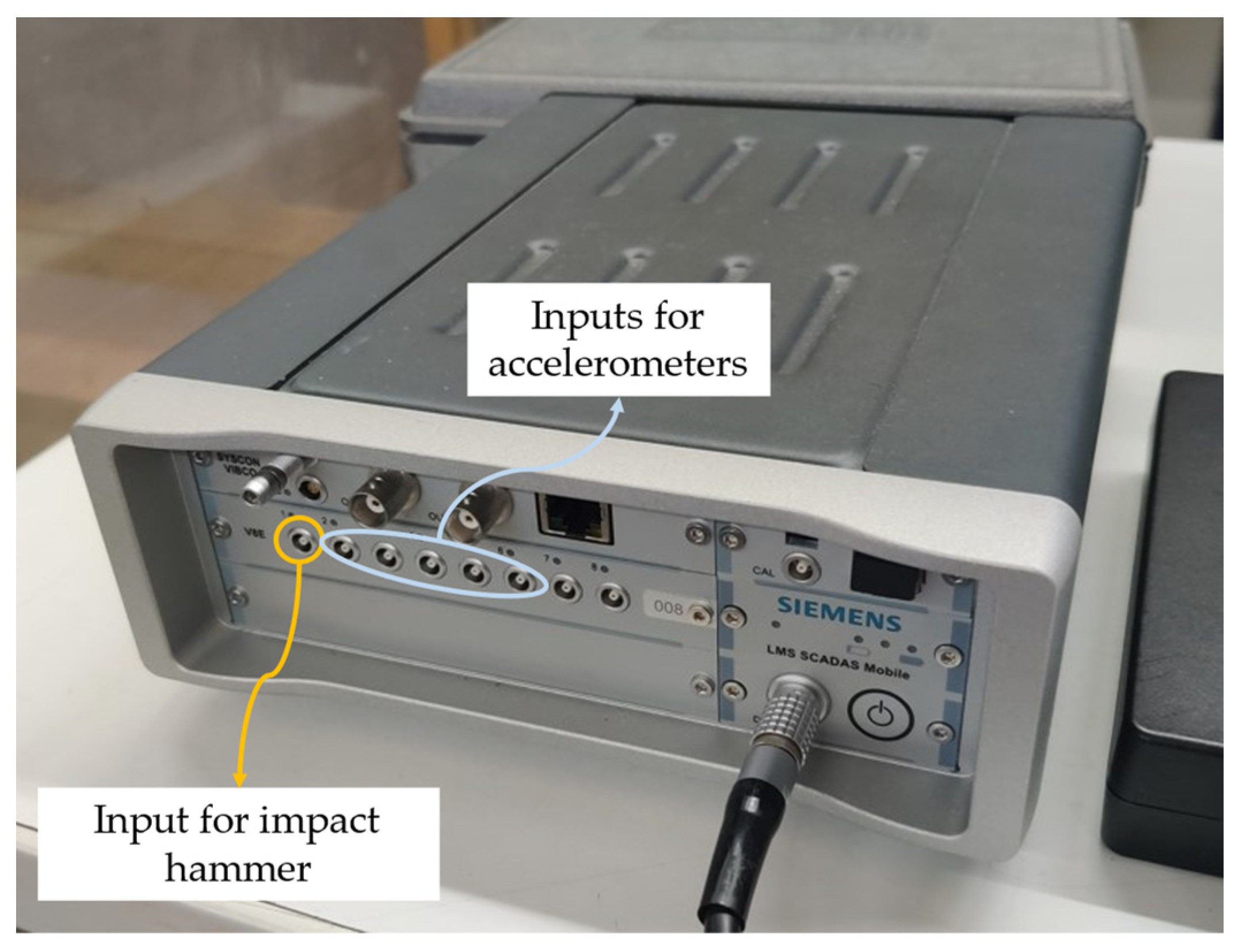
• $S_{fv}\left(\omega \right)$ is the cross-spectrum between the vibration acceleration (i.e., accelerometer signal) and the force (i.e., load cell signal).
• $S_{ff}\left(\omega \right)$ is the auto-spectrum of the input force.

The vibrations map is obtained by plotting the amplitude of the H₁ function in correspondence with the structure resonances. The Polymax algorithm was used for this aim; it estimates the modal parameters in the frequency domain depending on the interpolation of FRFs through fractional polynomial functions.

Hence, diverse strategies were implemented for the comparison between intact and damaged conditions.

At first, changes in terms of both natural vibration frequency (f_n) and loss factor (η) were computed, as reported in (2) and (3), respectively.

$$∆f_n=(f_n^{td}-f_n^{t0})/f_n^{t0}\times 100$$

(2)

where:

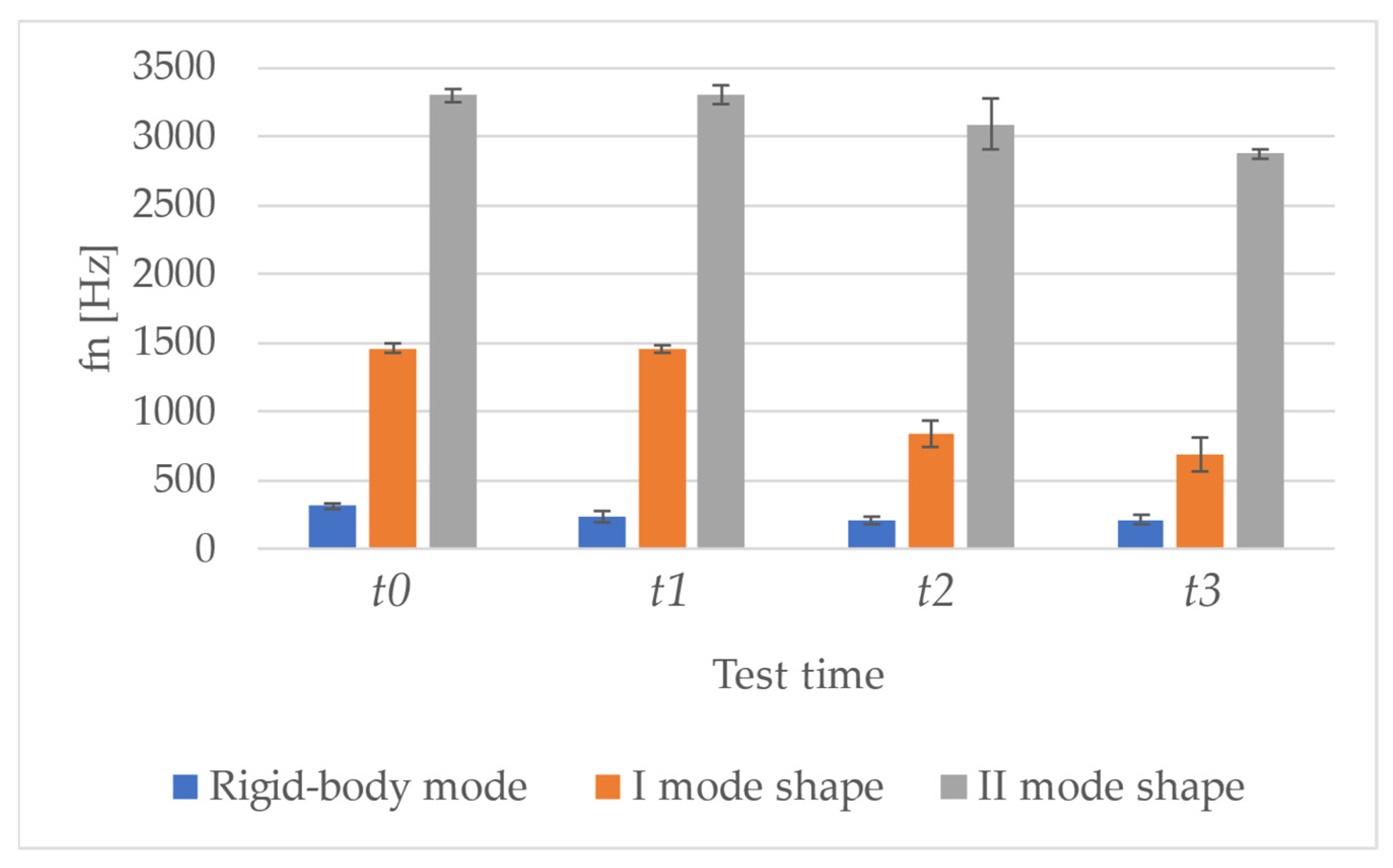
• $f_n^{t0}$ is the natural frequency at t0 (intact specimen).
• $f_n^{td}$ is the natural frequency at different test times (damaged specimen, i.e., t1, t2, and t3).

$$∆\eta =({\eta }^{td}-{\eta }^{t0})/{\eta }^{t0}\times 100$$

(3)

where:

• ${\eta }^{t0}$ is the loss factor at t0 (intact specimen).
• ${\eta }^{td}$ is the loss factor at different test times (damaged specimen, i.e., t1, t2, and t3).

Also, the MAC between mode shapes was evaluated at each test time (tj) related to damaged element with respect to t0 (i.e., intact element) on the same specimen and for the same mode. Indeed, the MAC is expected to decrease with damage occurrence.

The subsequent analyses were performed exclusively on the I mode shape of the analysed beams (excluding rigid-body and II mode shape); indeed, in practice, the modal curvature can be computed effectively only for low-order mode shapes [22], given the limited number of measurement points (i.e., 20 DOFs in the present study).

Modal curvatures (${\phi }^{″}$) were computed as the second derivative of the related mode shapes; being the latter complex, also the former will be. However, the main informative content is in the real part of the signal, as it is possible to verify in the example reported in Figure 6.

Given the noise typical of experimental data, plus the discrete measurement points, at first, data were oversampled (i.e., the number of points in the signal was increased, with an oversampling factor of ×5 used to increase the original sample rate) in order to have more points on for the computation of modal curvature (since experimental data are acquired on discrete points and the error increases with the distance between two consecutive points [45]). Hence, the central difference method was used to approximate the second derivative of the mode shape, since this method works well for smooth signals, as those obtained increasing the number of the points in the signal.

Then, the cuspid caused by the damage occurrence was evidenced through CWT-based analysis; curvatures were interpolated considering 200 points and Equation (4) was used to extract the real part of the mode shape curvature, being the real part of mode shape more informative [47].

$${\phi }_{comb}^{″}=\left|{\phi }^{″}\right|\times cos\left(\angle {\phi }^{″}\right)$$

(4)

where:

• $\left|{\phi }^{″}\right|$ is the modulus of the modal curvature (${\phi }^{″}$)
• $\angle {\phi }^{″}$ is the phase of the modal curvature (${\phi }^{″}$)

The continuous wavelet transform essentially makes a convolution of the input signal with functions derived from a mother wavelet (continuous in both time and frequency domains) that is scaled and translated in time. In this study the cwt function of MATLAB^® (R2023b) was employed; it uses the Morse wavelet. The symmetry (γ) and the time-bandwidth product parameters were set at 2 and 2.5, respectively, empirically selecting them to highlight the curvature formation in the mode shape. The absolute value obtained from this process can be plotted in function of time and frequency, obtaining the so-called scalogram. Then, the image was binarized using the global threshold method; hence, a binary image was created exploiting Otsu’s method [59], which creates a global threshold minimizing the intraclass variance of black/white pixels subjected to the threshold. Then, the area of the high-valued pixels was computed, and the values obtained at the different test times were compared.

Finally, three different damage indices were calculated. DI_curv, as reported in (5), is the sum of the absolute differences in modal curvature between each test time related to the damaged specimen with respect to the intact specimen (assessed at t0), where each difference is normalized with respect to the absolute value of the curvature maximum value at t0.

$${DI}_{curv}=\sum _{i=1}^N\frac{\left|{{\phi }^{″}}_{tx}-{{\phi }^{″}}_{t0}\right|}{max\left|{{\phi }^{″}}_{t0}\right|}$$

(5)

where:

• ${{\phi }^{″}}_{tx}$ is the modal curvature computed at the t_x test time (i.e., t1, t2, and t3).
• ${{\phi }^{″}}_{t0}$ is the modal curvature computed at t0 (intact specimen).

Substantially, this index recalls that proposed by Pranno et al. [22] (i.e., CDF), normalizing it with respect to $max\left|{{\phi }^{″}}_{t0}\right|.$ However, in this study, only the I-mode shape was considered.

A second damage-related index, DI_CWT, was defined based on CWT-based analysis. At first, the image obtained from CWT computation was binarized according to an automated threshold defined according to Otsu’s method [59]. Then, the area of the high CWT coefficients in the binarized image was computed and the value was normalized with respect to the area obtained for t0, as reported in (6).

$${DI}_{CWT}=\frac{{\left.\sum _{i=1}^N(pixel=1)\right|}_{tx}}{{\left.\sum _{i=1}^N(pixel=1)\right|}_{t0}}$$

(6)

While DI_curv is expected to increase with damage, since changes in modal curvature will be more significant, DI_CWT should decrease (i.e., smaller high pixel area).

A third damage index, DI_global, was defined, by combining the previous ones, as reported in (7).

$${DI}_{global}=\frac{{DI}_{curv}}{{DI}_{CWT}}$$

(7)

This index is expected to increase with damage and its importance since the numerator should increase while the denominator should decrease with damage occurrence and also with increasing severity. In this way, both changes in modal curvatures inferred from CWT-based analysis are included, making this index more robust.

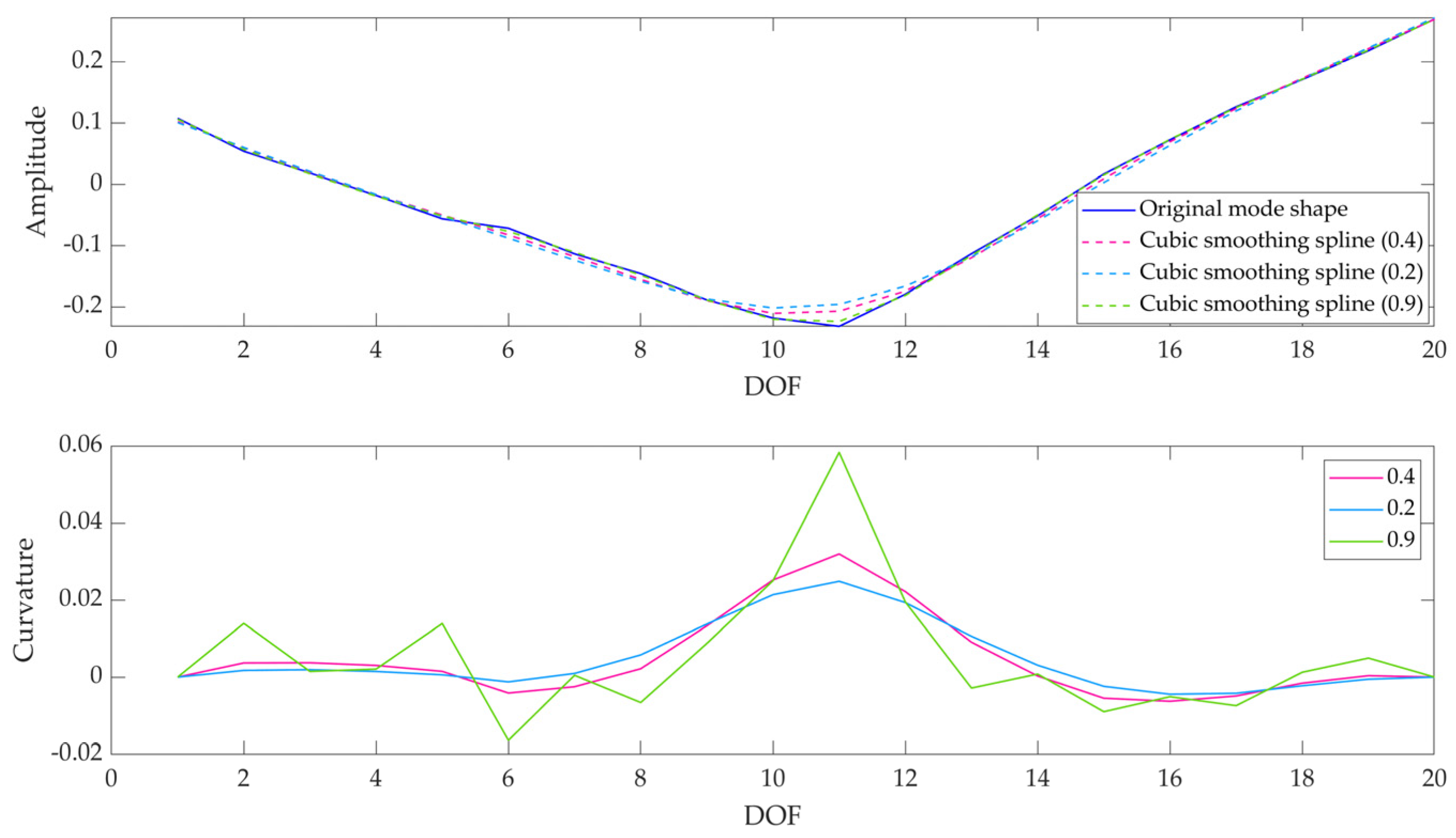
2.2. Sensitivity Analysis to Data Processing Parameters

A sensitivity analysis was performed to investigate the sensitivity of the results in terms of damage indices to some data processing parameters, in particular:

• Interpolation smoothing factor.
• Oversampling factor.

The first factor is involved in the cubic spline interpolation employed before the computation of modal curvature. Indeed, without interpolating the mode shapes the discontinuity due to the presence of damage would be more evident; on another hand, the presence of noise in experimental data would provide a bad-quality baseline signal (i.e., modal curvature related to the intact specimen). Hence, a compromise is needed between the aim of obtaining good quality data and the desire to clearly detect the damage-related discontinuity. In fact, the literature states that modal curvature computation is effective only with smooth signals [45]. Regarding oversampling, the step is needed to have a lower distance between points, thus reducing the noise due to limited experimental data [45], which in this way are increased in post-processing by multiplying the original sample rate by a certain factor.

Therefore, a sensitivity analysis was performed on specimen data (i.e., specimen A) and the tested values for the two considered variables are reported in

Table 2. Sensitivity analysis parameters: values considered for smoothing and oversampling factors.

Variable	Values
Smoothing factor	0.20
	0.40
	0.90
Oversampling factor	×2
	×5
	×10

. The effect of the selection of different processing parameters was evaluated in terms of damage-related indices.

3. Results and Discussion

The flexural strength measured on the dedicated specimens was equal to 12 kN. However, due to the intrinsic variability of concrete, the tested beams conveyed different fracture loads (13.5 ± 0.89, reported as mean ± standard deviation), as illustrated in

Table 3. Fracture loads under flexure for each tested specimen.

Specimen	Fracture Load [kN]
A	13.1
B	13.1
C	15.2
G	13.8
H	13.5
I	12.3

.

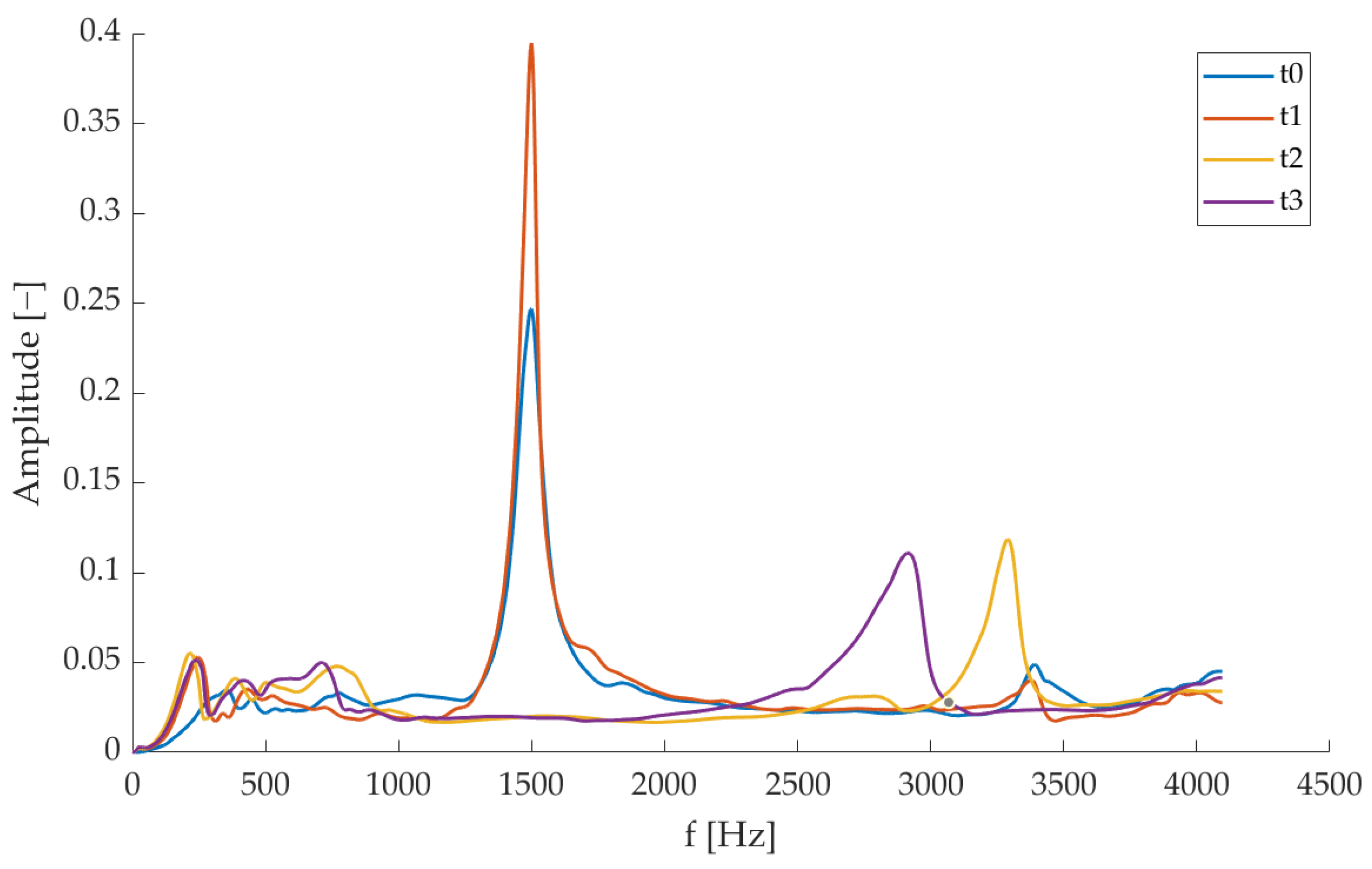
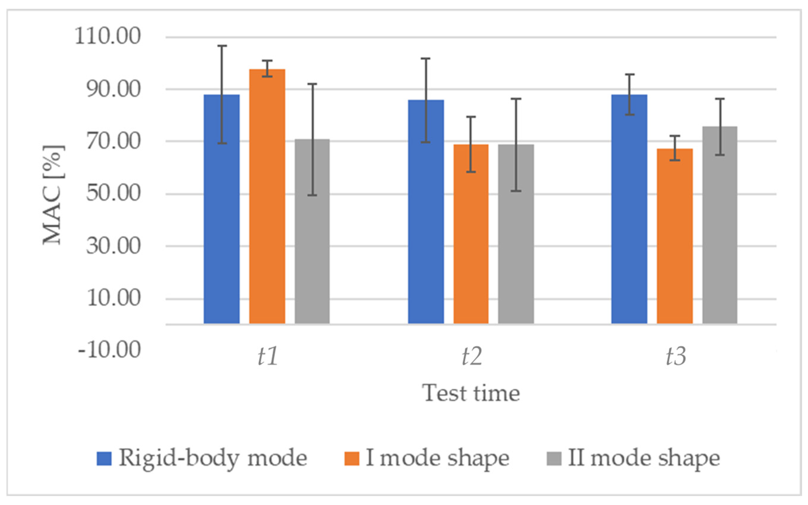
3.1. Modal Parameters

The results from the modal analysis are reported in terms of natural vibration frequency (

Table 4. Natural vibration frequency values for each tested specimen (A, B, C, G, H, and I) at each test time (t0, t1, t2, and t3) and related percentage variations with respect to undamaged condition (t0).

Specimen	Test Time	fn (Δfn [%]) [Hz]
		Mode Shape
		Rigid-Body	I	II
A	t0	341 (-)	1487 (-)	3371 (-)
	t1	237 (−30.44)	1488 (−0.07)	3383 (−0.35)
	t2	218 (−36.12)	796 (−46.47)	3265 (−3.14)
	t3	210 (−38.48)	715 (−51.92)	2888 (−14.34)
B	t0	329 (-)	1446 (-)	3273 (-)
	t1	294 (−10.64)	1442 (−0.34)	3295 (−0.67)
	t2	249 (−24.20)	748 (−48.30)	3172 (−3.09)
	t3	258 (−21.64)	481 (−66.73)	2871 (−12.28)
C	t0	343 (-)	1467 (-)	3315 (-)
	t1	285 (−16.91)	1462 (−0.33)	3331 (−0.48)
	t2	203 (−40.82)	794 (−45.88)	3170 (−4.37)
	t3	259 (−24.52)	597 (−59.33)	2884 (−13.00)
G	t0	289 (-)	1519 (-)	3338 (-)
	t1	235 (−18.69)	1487 (−2.10)	3330 (−0.26)
	t2	199 (−31.04)	767 (−49.50)	2687 (−19.52)
	t3	212 (−26.48)	870 (−42.73)	2861 (−14.31)
H	t0	303 (-)	1441 (-)	3280 (-)
	t1	159 (−47.47)	1425 (−1.10)	3319 (−1.18)
	t2	160 (−47.19)	951 (−33.98)	3127 (−4.66)
	t3	181 (−40.36)	786 (−45.41)	2942 (−10.31)
I	t0	300 (-)	1403 (-)	3224 (-)
	t1	215 (−28.52)	1412 (−0.63)	3173 (−1.58)
	t2	206 (−31.41)	1002 (−28.59)	3142 (−2.54)
	t3	175 (−41.79)	708 (−49.55)	2829 (−12.25)

) and loss factor (

Table 5. Loss factor (η) values for each tested specimen (A, B, C, G, H, and I) at each test time (t0, t1, t2, and t3) and related percentage variations (Δη) with respect to undamaged condition (t0).

Specimen	Test Time	η (Δη [%]) [%]
		Mode Shape
		Rigid-Body	I	II
A	t0	10.76 * (-)	1.70 (-)	0.69 (-)
	t1	2.48 (−76.99 *)	1.15 (−32.35 *)	0.86 (24.35)
	t2	3.99 (−62.96 *)	3.69 (117.09)	1.17 (69.42)
	t3	12.35 (14.80)	3.98 (134.12)	2.23 (223.37)
B	t0	9.45 (-)	1.98 (-)	0.70 (-)
	t1	10.31 (9.05)	2.67 (35.35)	0.95 (34.86)
	t2	17.45 (84.57)	9.23 (367.19)	1.42 (102.19)
	t3	20.85 (120.52)	11.44 (479.27)	2.25 (219.69)
C	t0	5.56 (-)	2.03 (-)	0.91 (-)
	t1	6.15 (10.55)	2.27 (11.97)	1.41 (54.93)
	t2	10.40 (87.05)	6.30 (210.58)	2.54 (179.82)
	t3	11.36 (104.25)	9.14 (350.61)	4.11 (353.01)
G	t0	9.34 (-)	1.59 (-)	0.78 (-)
	t1	9.34 (0.00)	2.00 (26.14)	0.78 (0.00)
	t2	14.75 (57.96)	7.76 (389.43)	2.22 (186.60)
	t3	19.12 (104.79)	9.56 (502.87)	3.05 (293.02)
H	t0	1.16 * (-)	1.46 * (-)	1.01 (-)
	t1	0.22 (−81.45 *)	0.84 (−42.12 *)	1.55 (52.82)
	t2	0.85 (−26.72)	1.73 (18.82)	2.67 (163.97)
	t3	2.38 (105.33)	3.11 (113.36)	2.30 (127.47)
I	t0	9.87 (-)	1.79 (-)	1.17 (-)
	t1	10.31 (4.51)	2.68 (49.76)	1.99 (70.08)
	t2	15.23 (54.29)	3.45 (92.79)	2.05 (75.21)
	t3	16.56 (67.78)	7.90 (341.55)	2.95 (152.13)

* Outliers.

) obtained for each test time (i.e., t0, t1, t2, and t3), and MAC values obtained correlating the mode shapes estimated for the three loading tests to the mode shapes estimated in the undamaged condition (i.e., t0) on the same specimen (

Table 6. MAC values for each tested specimen (A, B, C, G, H and I) considering different test times (i.e., t1, t2, and t3) with respect to t0 (i.e., undamaged conditions).

Specimen	Test Time	MAC [%]
		Mode Shape
		Rigid-Body	I	II
A	t0	93.81	90.97	29.19
	t1	93.14	78.19	59.84
	t2	87.50	72.85	57.59
	t3	98.63	98.63	89.64
B	t0	94.44	64.21	84.20
	t1	85.31	66.86	89.10
	t2	97.47	99.67	82.71
	t3	93.60	50.40	86.58
C	t0	92.14	60.88	82.65
	t1	97.13	99.31	84.85
	t2	84.74	64.44	34.35
	t3	94.96	74.40	83.07
G	t0	46.34	99.36	81.35
	t1	50.94	80.74	72.58
	t2	72.75	64.52	75.62
	t3	94.78	99.41	57.18
H	t0	97.81	76.38	75.40
	t1	95.61	65.20	66.77
	t2	93.81	90.97	29.19
	t3	93.14	78.19	59.84
I	t0	87.50	72.85	57.59
	t1	98.63	98.63	89.64
	t2	94.44	64.21	84.20
	t3	85.31	66.86	89.10

).

At first, the FRFs obtained in terms of Inertance were analysed to identify the low-frequency modes; in this range rigid-body mode, I, and II mode shapes were identified, as reported in Figure 7 for t0 test time (undamaged specimens). It is possible to notice a certain variability in the dynamic behaviour of the tested specimens. If the natural vibration frequency of the I mode shape is considered (I is the most evident one), a variability of approximately 100 Hz can be evidenced. Hence, if a variation of that order is observed, it cannot be attributed to external factors (e.g., damage occurrence), since it falls within the specimen variability range. No significant differences can be evidenced between sensorized (i.e., A, B, and C) and not-sensorized (i.e., G, H, and I) specimens.

Changes caused by cracking phenomena (Figure 8) are more easily visible in the I mode shape, whose natural vibration frequency is reduced by (42.12 ± 7.91)% at t2 (first crack formation) and practically halved at t3, with a decrease of (52.61 ± 8.20)%. It is possible to recognize a cuspid in the mode shape (Figure 9), highlighting the presence of damage in the specimen mid-line. This feature can be further evidenced through the computation of modal curvature, as reported in Section 3.2. Concerning the II mode shape, it is worth noting that at t0 its natural vibration frequency was probably at higher frequencies; then, with the occurrence of cracks, the natural frequency decreased, re-entering the observed frequency band (i.e., 4096 Hz). However, that mode presents a nodal line in correspondence with the beam mid-line, hence the damage is hardly identifiable. For this reason, the remaining part of the damage-identification procedure was focused on the I mode shape.

Being the vibrational tests conducted after the load removal, it should be stressed that the differences in results at t2 and t3 could be not always very evident since the crack partially re-closes before the impact test execution.

Regarding the first crack formation (i.e., t2), changes in the natural vibration frequency (Figure 8) are equal to (–42.12 ± 7.91)% for the I mode shape; this is also visible from the Sum FRFs (Figure 10). When the crack aperture is widened until approximately 1 mm, the changes achieve (−52.61 ± 8.20)%; in particular, it can be noticed that the natural vibration frequency passes from a mean value of 1461 Hz (±37 Hz) at t0 to 843 Hz (±97 Hz) at t2 and to 693 Hz (±126 Hz) at t3. However, the results are not consistent among all the tested specimens, since vibrational tests were performed after having removed the external load, so the crack has the possibility of partially closing, as mentioned above. Even if beyond the scope of this paper, it is worth underlining that the crack aperture was assessed through a previous measurement procedure based on vision techniques [60] and the measured values were in the range of 0.3–0.6 mm; this confirms the partial crack closure after the load removal. Furthermore, being the structure reinforced, the damage is diffused.

Concerning the loss factor (Table 4), given the presence of the crack and therefore the enhancement of the vibration loss through the propagation into the fracture itself, it is possible to observe an increasing trend with test times (Figure 11). In particular, η value passes from (7.69 ± 3.35)% at t0 to (13.77 ± 6.11)% at t3 for rigid-body shape, from (1.76 ± 0.20)% at t0 to (7.52 ± 3.01)% at t3 for I mode shape, and from (0.88 ± 0.17)% at t0 to (2.82 ± 0.67)% at t3 for II mode shape. However, it is worth noting the high variability among specimens, but this is in line with what is expected, also from the literature [36].

Analysing the MAC values (Table 6), a decrease in correlation at tx with respect to t0 test time (i.e., same specimen in undamaged conditions) is expected over test times, since the formation of cracks makes the mode shapes change. Indeed, this behaviour is well evident only for the I mode shape, since both rigid-body shape and II mode shape show compatible values, for example, at t1 and t2. It is a different matter for the comparison between t2 and t3, given that the analyses were performed after having removed the load, which let the crack partially close, as mentioned above. The mean trends and their variability are reported in Figure 12.

Since the modification is more evident for the I mode shape (e.g., the rigid-body shape proves to be insensitive to damages, showing no deflection), the successive analyses (regarding both modal curvatures and CWT-base analyses) were focused on it; indeed, if the mode shapes are observed, at t3 it is clear that the beams are broken and vibrate as two quasi-separate objects and this behaviour partially shows at t2 (Figure 9).

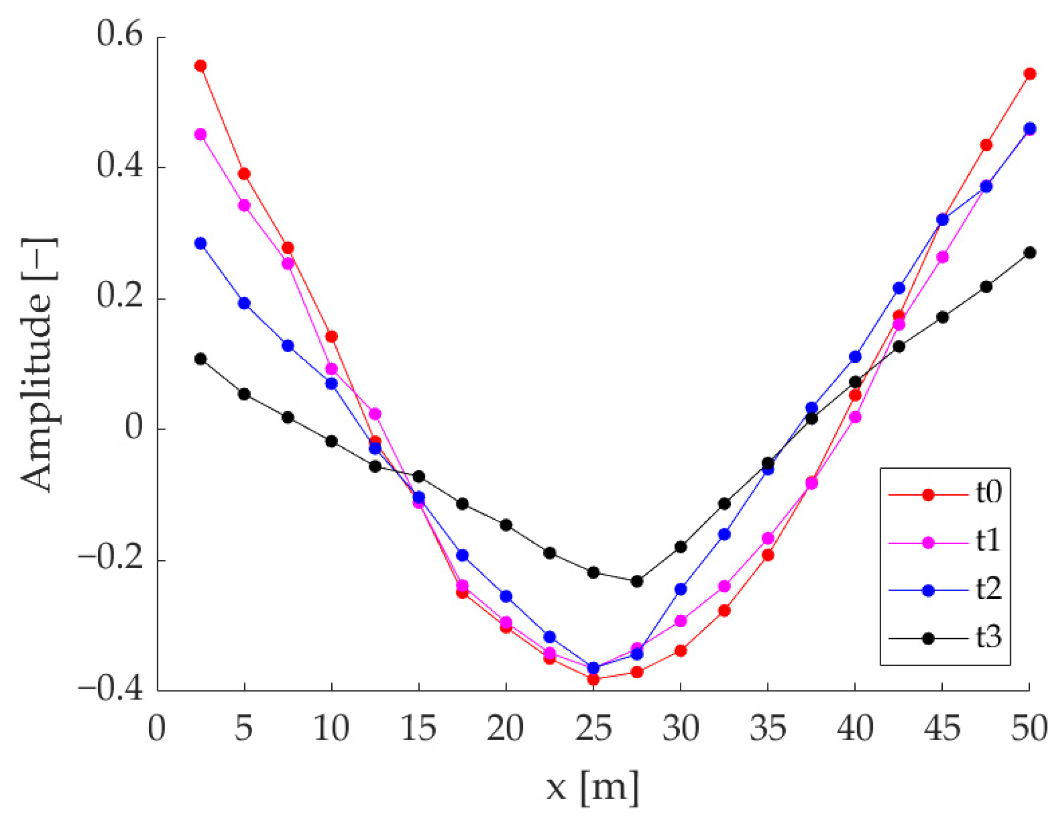
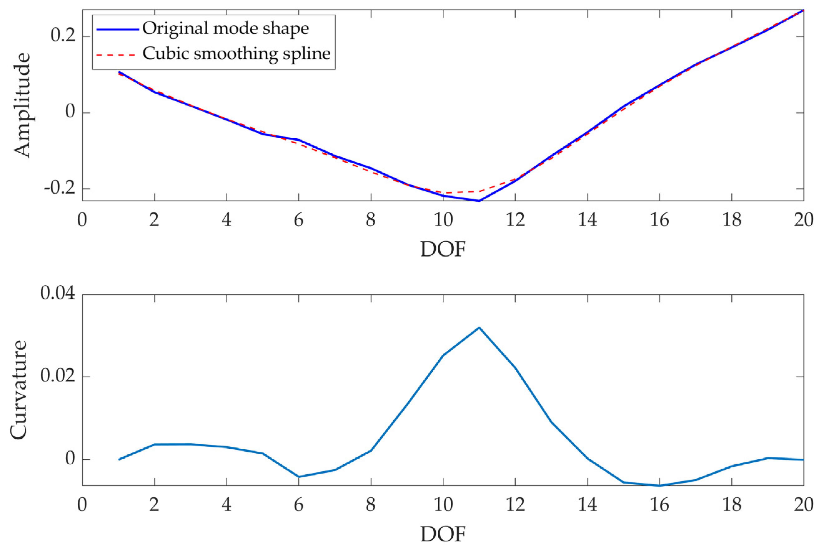
3.2. Modal Curvatures and CWT-Based Analysis

The computation of modal curvatures allows to highlight of the cuspid formation in correspondence with the damage; it is worth underlining that the main crack forms in the specimen centerline, hence the damage is hardly identifiable from mode shapes presenting a nodal line in this area (e.g., II mode shape). This further justifies the choice of performing this analysis only on I mode shape (excluding rigid-body mode).

An example of the modal curvature computation, referred to as specimen A, is reported in Figure 13; the preliminary smoothing of the mode shape (through a cubic spline interpolation with a smoothing factor of 0.4) allows to obtain a less noisy curvature. The comparison among curvatures obtained at different test times is reported in Figure 14 (where curvatures are interpolated with a factor of 100, hence 2000 points are obtained); the cuspid appears with the crack formation at t2 and the morphology is clearly distinguishable from t0 (i.e., undamaged conditions). The application of CWT makes its objective identification easily feasible, as can be observed in Figure 15; indeed, the binarization of the image (Figure 16) leads to the definition of an area shape immediately referring to the cuspid and, hence, to the damage occurrence.

3.3. Damage Related Indices

As a synthetic way to identify and represent the damaged status of a cement-based structural element, the authors evaluated different indices, namely DI_curv, DI_CWT, and DI_global (see Section 3 for details). The results obtained on all the tested specimens for each test time are reported in

Table 7. Damage-related indices for each tested specimen (A, B, C, G, H, and I) at each test time (t1, t2, and t3).

Specimen	Test Time	Damage Indices
		DIcurv	DICWT	DIglobal
A	t1	4.98	1.01	4.94
	t2	8.74	0.83	10.53
	t3	8.66	0.82	10.59
B	t1	3.93	1.17	3.36
	t2	7.49	0.89	8.44
	t3	7.82	0.90	8.69
C	t1	2.61	0.96	2.73
	t2	8.35	0.81	10.33
	t3	8.90	1.00 *	8.92 *
G	t1	2.13	0.87	2.44
	t2	6.03 *	0.82	7.37 *
	t3	5.03	0.85 *	5.93
H	t1	3.61	1.08	3.36
	t2	7.07	0.92	7.65
	t3	9.13	0.90	10.16
I	t1	3.64	1.17	3.10
	t2	6.57	0.86 *	7.65 *
	t3	7.49	0.89	8.44

* Outliers.

and are summarized in Figure 17; it can be observed that the values obtained for t2 and t3 test times fall in compatible measurement ranges, meaning that the two conditions cannot be distinguished. This is probably linked to the fact that the vibrational analyses were performed after the load removal, letting the crack partially close. On the contrary, there is a significant variation between the indices obtained at t1 (i.e., 90% of fracture load) and the values after damage occurrence (i.e., at t2 and t3). The first crack formation (i.e., t2) can be promptly detected, signalling an alteration of the dynamic behaviour of the element; this proves that the proposed assessment strategy is effective and adequately sensitive to the occurrence of damage. Hence, the results confirm the possibility of discriminating between intact (i.e., t1) and damaged (i.e., t2 and t3) conditions, but further investigations are needed to distinguish among different levels of damage (e.g., between t2—crack formation—and t3—crack aperture of 1 mm—conditions).

3.4. Sensitivity Analysis

The results in terms of the sensitivity of damage-related indices to data processing variables, namely smoothing factor, and oversampling factor, are reported in

Table 8. Results of sensitivity analysis.

Variable	Values	Test Time	Damage Indices
			DIcurv	DICWT	DIglobal
Smoothing factor (with oversampling factor ×5)	0.20	t1	2.88	1.01	2.85
		t2	6.82	0.94	7.29
		t3	6.39	0.95	6.75
	0.40	t1	4.98	1.01	4.94
		t2	8.74	0.83	10.53
		t3	8.66	0.82	10.59
	0.90	t1	8.09	0.61	13.22
		t2	11.26	1.01	11.17
		t3	11.36	1.28	8.68
Oversampling factor (with smoothing factor 0.4)	×2	t1	4.98	1.02	4.85
		t2	8.74	0.85	10.34
		t3	8.66	0.81	10.69
	×5	t1	4.98	1.01	4.94
		t2	8.74	0.83	10.53
		t3	8.66	0.82	10.59
	×10	t1	4.98	1.01	4.92
		t2	8.74	0.84	10.44
		t3	8.66	0.82	10.51

. It is worth noting that the sensitivity analysis has been performed separately on the two variables. It is possible to observe that the change of smoothing factor has a significant effect on all the damage-related indices (in case of DI_curv, with an almost constant sensitivity, varying in the range of 2.2–2.6 depending on the test time, as it can be deduced from Table 8); when it is halved (passing from 0.4 to 0.2), DI_curv decreases of approximately 26%, DI_CWT increases of about 16%, and DI_global decreases of about 36% at t3 test time. The DI_CWT index trend is no longer monotonically decreasing as expected since the smoothing operation is too aggressive and the cuspid is no more identifiable. On the other hand, considering the softest smoothing operation (i.e., smoothing factor equal to 0.9), it is possible to notice that this is not sufficient to obtain a good quality baseline curvature at t0 (Figure 18). The damage is no longer identifiable through none of the indices (their trends are opposed compared to the expected ones)—even if considering only t3 test time the cuspid would be more evident (but at the expense of signal quality, especially at t0). Therefore, a smoothing factor equal to 0.40 can be considered adequate for our purposes (a comparison can be observed in Figure 19). Concerning the oversampling factor, its effect is slightly on DI_CWT and, hence, DI_global indices. No significant changes can be evidenced, hence a ×5 oversampling factor can be considered a good compromise to have a good quality signal and limited computational load at the same time.

4. Conclusions

The experimental modal analysis performed in this study allowed us to identify the crack formation in the tested scaled concrete beams; in particular, the damage occurrence causes (i) a decrease in natural vibration frequency and (ii) an increase of the loss factor (since the element rigidity decreases). Moreover, a decrease in terms of MAC between the mode shapes estimated for damaged samples and the mode shapes estimated for the corresponding undamaged samples can be observed with the damage occurrence, due to the change of the mode shapes morphology. The variations of both modal parameters and mode shapes can be highlighted through the computation of the related modal curvatures (after proper signal pre-processing to enhance SNR, considering the sensitivity of results towards data processing parameters, in particular, smoothing factor); moreover, specific processing techniques, namely CWT, can help in objectively identifying the formation of discontinuities (e.g., cuspid) in the modal curvatures, which are characteristic of the induced damage. Finally, synthetic damage indices can be used to provide a global indication of the health status of a cement-based element or structure.

In practical in-field applications, if the measurements at t0 (undamaged conditions) are not available, a validated numerical model could provide the baseline modal parameters of the structure. For example, a comparison between the experimental curvature and the theoretical one (numerically obtained) could be carried out to evaluate the presence of possible damages in the structure. Indeed, the diagnostic methods based on a comparison with baseline data are less tricky, whereas analysing only experimental curvatures may require more complex computational methods to identify eventual damages. Specific thresholds should be considered since they are problem-dependent values. Moreover, it is worth underlining the importance of data quality, since noisy data hinder the computation of reliable modal curvatures; smoothing techniques can be applied before deriving the signal to this aim, but this could mask also the discontinuities linked to the damage occurrence. Hence, a good compromise between the use of filtering and smoothing techniques to enhance SNR and the need to preserve damage-related discontinuities should be pursued. Nevertheless, data processing techniques are pivotal when dealing with experimental data, which are inevitably affected by noise and are more demanding compared to numeric results derived from synthetic models. Data processing parameters related to smoothing and oversampling techniques enhancing the signal quality can influence the final results (as evidenced by the sensitivity analysis performed in this work), hence they should be properly selected. Moreover, it is important to stress the fact that the considered frequency band directly influences the mode shapes that can be investigated, which will be inevitably less than those observable in the case of numerical models.

Finally, in the future more indices (possibly inferred from multidomain signals) could be combined to increase the method sensitivity to damages, also thanks to data fusion techniques. In addition, the suitability of the method for regular structural monitoring could be evaluated; in this context the use of Laser Doppler Vibrometry (LDV) could be evaluated for in-field applications, to enable the vibrational analysis even in operating conditions and in (near) real-time (e.g., during the application of a load). In this way, the proposed strategy could become a monitoring technique, without the limits of single (or at most periodic) inspections.

References

1. Sofi, A.; Regita, J.J.; Rane, B.; Lau, H.H. Structural health monitoring using wireless smart sensor network–An overview. Mech. Syst. Signal Process. 2022, 163, 108113. [Google Scholar] [CrossRef]
2. Limongelli, M. Frequency response function interpolation for damage detection under changing environment. Mech. Syst. Signal Process. 2010, 24, 2898–2913. [Google Scholar] [CrossRef]
3. Hu, W.-H.; Tang, D.-H.; Teng, J.; Said, S.; Rohrmann, R.G. Structural Health Monitoring of a Prestressed Concrete Bridge Based on Statistical Pattern Recognition of Continuous Dynamic Measurements over 14 years. Sensors 2018, 18, 4117. [Google Scholar] [CrossRef] [PubMed]
4. Ietka, I.; Moutinho, C.; Pereira, S.; Cunha, A. Structural Monitoring of a Large-Span Arch Bridge Using Customized Sensors. Sensors 2023, 23, 5971. [Google Scholar] [CrossRef] [PubMed]
5. Ye, C.; Kuok, S.C.; Butler, L.J.; Middleton, C.R. Implementing bridge model updating for operation and maintenance purposes: Examination based on UK practitioners’ views. Struct. Infrastruct. Eng. 2022, 18, 1638–1657. [Google Scholar] [CrossRef]
6. Kamariotis, A.; Chatzi, E.; Straub, D. A framework for quantifying the value of vibration-based structural health monitoring. Mech. Syst. Signal Process. 2023, 184, 109708. [Google Scholar] [CrossRef]
7. Mesquita, E.; Antunes, P.; Coelho, F.; André, P.; Arêde, A.; Varum, H. Global overview on advances in structural health monitoring platforms. J. Civ. Struct. Health Monit. 2016, 6, 461–475. [Google Scholar] [CrossRef]
8. Alavi, A.H. The Rise of Smart Cities Advanced Structural Sensing and Monitoring Systems; Elsevier: Amsterdam, The Netherlands, 2022. [Google Scholar]
9. Mobili, A.; Cosoli, G.; Giulietti, N.; Chiariotti, P.; Bellezze, T.; Pandarese, G.; Revel, G.; Tittarelli, F. Biochar and recycled carbon fibres as additions for low-resistive cement-based composites exposed to accelerated degradation. Constr. Build. Mater. 2023, 376, 131051. [Google Scholar] [CrossRef]
10. Ozelim, L.C.d.S.M.; Borges, L.P.d.F.; Cavalcante, A.L.B.; Albuquerque, E.A.C.; Diniz, M.d.S.; Góis, M.S.; da Costa, K.R.C.B.; de Sousa, P.F.; Dantas, A.P.D.N.; Jorge, R.M.; et al. Structural Health Monitoring of Dams Based on Acoustic Monitoring, Deep Neural Networks, Fuzzy Logic and a CUSUM Control Algorithm. Sensors 2022, 22, 2482. [Google Scholar] [CrossRef]
11. Gayakwad, H.; Thiyagarajan, J.S. Structural Damage Detection through EMI and Wave Propagation Techniques Using Embedded PZT Smart Sensing Units. Sensors 2022, 22, 2296. [Google Scholar] [CrossRef]
12. Klun, M.; Zupan, D.; Lopatič, J.; Kryžanowski, A. On the Application of Laser Vibrometry to Perform Structural Health Monitoring in Non-Stationary Conditions of a Hydropower Dam. Sensors 2019, 19, 3811. [Google Scholar] [CrossRef]
13. Li, Z.; Lin, W.; Zhang, Y. Drive-by bridge damage detection using Mel-frequency cepstral coefficients and support vector machine. Struct. Health Monit. 2023, 22, 3302–3319. [Google Scholar] [CrossRef]
14. Giordano, P.F.; Limongelli, M.P. The value of structural health monitoring in seismic emergency management of bridges. Struct. Infrastruct. Eng. 2020, 18, 537–553. [Google Scholar] [CrossRef]
15. Wang, J.; You, H.; Qi, X.; Yang, N. BIM-based structural health monitoring and early warning for heritage timber structures. Autom. Constr. 2022, 144, 104618. [Google Scholar] [CrossRef]
16. Mancini, A.; Cosoli, G.; Galdelli, A.; Violini, L.; Pandarese, G.; Mobili, A.; Blasi, E.; Tittarelli, F.; Revel, G.M. A monitoring platform for the built environment: Towards the development of an early warning system in a seismic context. In Proceedings of the 2023 IEEE International Workshop on Metrology for Living Environment (MetroLivEnv), Milano, Italy, 29–31 May 2023; pp. 102–106. [Google Scholar]
17. Xiao, F.; Zhu, W.; Meng, X.; Chen, G.S. Parameter Identification of Frame Structures by considering Shear Deformation. Int. J. Distrib. Sens. Netw. 2023, 2023, 6631716. [Google Scholar] [CrossRef]
18. Xiao, F.; Sun, H.; Mao, Y.; Chen, G.S. Damage identification of large-scale space truss structures based on stiffness separation method. Structures 2023, 53, 109–118. [Google Scholar] [CrossRef]
19. Zhang, C.; Mousavi, A.A.; Masri, S.F.; Gholipour, G.; Yan, K.; Li, X. Vibration feature extraction using signal processing techniques for structural health monitoring: A review. Mech. Syst. Signal Process. 2022, 177, 109175. [Google Scholar] [CrossRef]
20. Li, X.; Guan, Y.; Law, S.; Zhao, W. Monitoring abnormal vibration and structural health conditions of an in-service structure from its SHM data. J. Sound Vib. 2022, 537, 109175. [Google Scholar] [CrossRef]
21. Zhi-Qian, X.; Jian-Wen, P.; Jin-Ting, W.; Fu-Dong, C. Improved approach for vibration-based structural health monitoring of arch dams during seismic events and normal operation. Struct. Control. Health Monit. 2022, 29, e2955. [Google Scholar] [CrossRef]
22. Pranno, A.; Greco, F.; Lonetti, P.; Luciano, R.; De Maio, U. An improved fracture approach to investigate the degradation of vibration characteristics for reinforced concrete beams under progressive damage. Int. J. Fatigue 2022, 163, 107032. [Google Scholar] [CrossRef]
23. Sadeghi, F.; Yu, Y.; Zhu, X.; Li, J. Damage identification of steel-concrete composite beams based on modal strain energy changes through general regression neural network. Eng. Struct. 2021, 244, 112824. [Google Scholar] [CrossRef]
24. Giordano, P.F.; Limongelli, M.P. Response-based time-invariant methods for damage localization on a concrete bridge. Struct. Concr. 2020, 21, 1254–1271. [Google Scholar] [CrossRef]
25. Salehi, M.; Rad, S.Z.; Ghayour, M.; Vaziry, M.A. A non model-based damage detection technique using dynamically measured flexibility matrix. Iran. J. Sci. Technol. Trans. Mech. Eng. 2011, 35, 137–149. [Google Scholar]
26. Bońkowski, P.A.; Bobra, P.; Zembaty, Z.; Jędraszak, B. Application of Rotation Rate Sensors in Modal and Vibration Analyses of Reinforced Concrete Beams. Sensors 2020, 20, 4711. [Google Scholar] [CrossRef]
27. Lin, H.-P. Direct and inverse methods on free vibration analysis of simply supported beams with a crack. Eng. Struct. 2004, 26, 427–436. [Google Scholar] [CrossRef]
28. Dessi, D.; Camerlengo, G. Damage identification techniques via modal curvature analysis: Overview and comparison. Mech. Syst. Signal Process. 2015, 52–53, 181–205. [Google Scholar] [CrossRef]
29. Jahangir, H.; Khatibinia, M.; Naei, M.M.M. Damage Detection in Prestressed Concrete Slabs Using Wavelet Analysis of Vi-bration Responses in the Time Domain. J. Rehabil. Civ. Eng. 2022, 10, 37–63. [Google Scholar] [CrossRef]
30. Dilena, M.; Morassi, A. Dynamic testing of a damaged bridge. Mech. Syst. Signal Process. 2011, 25, 1485–1507. [Google Scholar] [CrossRef]
31. Cao, M.-S.; Xu, W.; Ren, W.-X.; Ostachowicz, W.; Sha, G.-G.; Pan, L.-X. A concept of complex-wavelet modal curvature for detecting multiple cracks in beams under noisy conditions. Mech. Syst. Signal Process. 2016, 76–77, 555–575. [Google Scholar] [CrossRef]
32. Koh, S.J.; Maalej, M.; Quek, S.T. Damage Quantification of Flexurally Loaded RC Slab Using Frequency Response Data. Struct. Health Monit. 2004, 3, 293–311. [Google Scholar] [CrossRef]
33. Voggu, S.; Sasmal, S. Dynamic nonlinearities for identification of the breathing crack type damage in reinforced concrete bridges. Struct. Health Monit. 2021, 20, 339–359. [Google Scholar] [CrossRef]
34. Radzieński, M.; Krawczuk, M.; Palacz, M. Improvement of damage detection methods based on experimental modal parameters. Mech. Syst. Signal Process. 2011, 25, 2169–2190. [Google Scholar] [CrossRef]
35. Hou, J.; Li, Z.; Zhang, Q.; Zhou, R.; Jankowski, Ł. Optimal Placement of Virtual Masses for Structural Damage Identification. Sensors 2019, 19, 340. [Google Scholar] [CrossRef] [PubMed]
36. Jiang, Y.; Wang, N.; Zhong, Y. A two-step damage quantitative identification method for beam structures. Measurement 2021, 168, 108434. [Google Scholar] [CrossRef]
37. Sazonov, E.; Klinkhachorn, P. Optimal spatial sampling interval for damage detection by curvature or strain energy mode shapes. J. Sound Vib. 2005, 285, 783–801. [Google Scholar] [CrossRef]
38. Cao, M.; Qiao, P. Novel Laplacian scheme and multiresolution modal curvatures for structural damage identification. Mech. Syst. Signal Process. 2009, 23, 1223–1242. [Google Scholar] [CrossRef]
39. Cao, M.; Xu, W.; Ostachowicz, W.; Su, Z. Damage identification for beams in noisy conditions based on Teager energy operator-wavelet transform modal curvature. J. Sound Vib. 2014, 333, 1543–1553. [Google Scholar] [CrossRef]
40. Chandrashekhar, M.; Ganguli, R. Damage assessment of composite plate structures with material and measurement uncertainty. Mech. Syst. Signal Process. 2016, 75, 75–93. [Google Scholar] [CrossRef]
41. Chandrashekhar, M.; Ganguli, R. Damage assessment of structures with uncertainty by using mode-shape curvatures and fuzzy logic. J. Sound Vib. 2009, 326, 939–957. [Google Scholar] [CrossRef]
42. Meruane, V.; Yanez, S.J.; Quinteros, L.; Flores, E.I.S. Damage Detection in Steel–Concrete Composite Structures by Impact Hammer Modal Testing and Experimental Validation. Sensors 2022, 22, 3874. [Google Scholar] [CrossRef]
43. Maia, N.; Silva, J.; Almas, E.; Sampaio, R. Damage Detection in Structures: From Mode Shape To Frequency Response Function Methods. Mech. Syst. Signal Process. 2003, 17, 489–498. [Google Scholar] [CrossRef]
44. Balageas, D.; Fritzen, C.P.; Güemes, A. Structural Health Monitoring; Wiley: Hoboken, NJ, USA, 2006; ISBN 9780470612071. [Google Scholar]
45. Jahangir, H.; Hasani, H.; Esfahani, M.R. Wavelet-based damage localization and severity estimation of experimental RC beams subjected to gradual static bending tests. Structures 2021, 34, 3055–3069. [Google Scholar] [CrossRef]
46. Quek, S.-T.; Wang, Q.; Zhang, L.; Ang, K.-K. Sensitivity analysis of crack detection in beams by wavelet technique. Int. J. Mech. Sci. 2001, 43, 2899–2910. [Google Scholar] [CrossRef]
47. Masciotta, M.; Pellegrini, D. Tracking the variation of complex mode shapes for damage quantification and localization in structural systems. Mech. Syst. Signal Process. 2021, 169, 108731. [Google Scholar] [CrossRef]
48. Bayissa, W.; Haritos, N.; Thelandersson, S. Vibration-based structural damage identification using wavelet transform. Mech. Syst. Signal Process. 2008, 22, 1194–1215. [Google Scholar] [CrossRef]
49. Jahangir, H.; Hasani, H.; Esfahani, M.R. Damage Localization of RC Beams via Wavelet Analysis of Noise Contaminated Modal Curvatures. J. Soft Comput. Civ. Eng. 2021, 5, 101–133. [Google Scholar] [CrossRef]
50. Sha, G.; Radzienski, M.; Soman, R.; Cao, M.; Ostachowicz, W.; Xu, W. Multiple damage detection in laminated composite beams by data fusion of Teager energy operator-wavelet transform mode shapes. Compos. Struct. 2020, 235, 111798. [Google Scholar] [CrossRef]
51. Anastasopoulos, D.; De Roeck, G.; Reynders, E.P. Influence of damage versus temperature on modal strains and neutral axis positions of beam-like structures. Mech. Syst. Signal Process. 2019, 134, 106311. [Google Scholar] [CrossRef]
52. Maes, K.; Van Meerbeeck, L.; Reynders, E.; Lombaert, G. Validation of vibration-based structural health monitoring on retrofitted railway bridge KW51. Mech. Syst. Signal Process. 2022, 165, 108380. [Google Scholar] [CrossRef]
53. Gordan, M.; Sabbagh-Yazdi, S.-R.; Ismail, Z.; Ghaedi, K.; Carroll, P.; McCrum, D.; Samali, B. State-of-the-art review on advancements of data mining in structural health monitoring. Measurement 2022, 193, 110939. [Google Scholar] [CrossRef]
54. Avci, O.; Abdeljaber, O.; Kiranyaz, S.; Hussein, M.; Gabbouj, M.; Inman, D.J. A review of vibration-based damage detection in civil structures: From traditional methods to Machine Learning and Deep Learning applications. Mech. Syst. Signal Process. 2021, 147, 107077. [Google Scholar] [CrossRef]
55. Sarmadi, H.; Yuen, K.-V. Structural health monitoring by a novel probabilistic machine learning method based on extreme value theory and mixture quantile modeling. Mech. Syst. Signal Process. 2022, 173, 109049. [Google Scholar] [CrossRef]
56. Guo, S.; Ding, H.; Li, Y.; Feng, H.; Xiong, X.; Su, Z.; Feng, W. A hierarchical deep convolutional regression framework with sensor network fail-safe adaptation for acoustic-emission-based structural health monitoring. Mech. Syst. Signal Process. 2022, 181, 109508. [Google Scholar] [CrossRef]
57. BSI 12390-5; 2019 Testing Hardened Concrete-Part 5: Flexural Strength of Test Specimens. BSI: London, UK, 2022.
58. Salehi, M.; Ziaei-Rad, S.; Ghayour, M.; Vaziri-Zanjani, M.A. A Structural Damage Detection Technique Based on Measured Frequency Response Functions. Contemp. Eng. Sci. 2010, 3, 215–226. [Google Scholar]
59. Otsu, N. A threshold selection method from gray-level histograms. IEEE Trans. Syst. Man Cybern. 1979, 9, 62–66. [Google Scholar] [CrossRef]
60. Giulietti, N.; Chiariotti, P.; Revel, G.M. Automated Measurement of Geometric Features in Curvilinear Structures Exploiting Steger’s Algorithm. Sensors 2023, 23, 4023. [Google Scholar] [CrossRef] [PubMed]
Figure 2. Mechanical press: (a) Frontal view; (b) Angular view.
Sensors 23 09292 g002
Figure 3. Specimen configuration for the impact test.
Sensors 23 09292 g003
Figure 4. Sequence of measurements with 5 accelerometers; 4 measurements are necessary to cover the whole specimen.
Sensors 23 09292 g004
Figure 5. Connection configuration for the measurement system (LMS SCADAS Mobile).
Sensors 23 09292 g005
Figure 6. Real (blue) and imaginary (red) parts of the I mode shape (specimen A).
Sensors 23 09292 g006
Figure 7. Sum FRFs obtained on the different specimens at t0 (intact beams). The three blue bands indicate the three considered mode shapes, namely rigid-body mode shape (left), I mode shape (centre), and II mode shape (right). The circular markers are related to their natural vibration frequencies.
Sensors 23 09292 g007
Figure 8. Natural vibration frequencies are reported as mean ± standard deviation at each test time for all the specimens.
Sensors 23 09292 g008
Figure 9. Example of I mode shape with cuspid formation due to crack (t2 and t3 test times)—specimen A.
Sensors 23 09292 g009
Figure 10. Sum FRFs at different test times (Specimen A).
Sensors 23 09292 g010
Figure 11. Loss factor values are reported as mean ± standard deviation at each test time for all the specimens.
Sensors 23 09292 g011
Figure 12. MAC values are reported as mean ± standard deviation at t1, t2, and t3 test times with respect to t0 for all the specimens.
Sensors 23 09292 g012
Figure 13. Modal curvature computation for I mode shape: mode shape (raw and smoothed) (top), and modal curvature (bottom)—(Specimen A, test time: t3).
Sensors 23 09292 g013
Figure 14. Comparison of I modal curvature computed at each test time (i.e., t0, t1, t2, and t3—Specimen A)—2000 points obtained through interpolated curvatures.
Sensors 23 09292 g014
Figure 15. Comparison of the CWTs scalograms of I modal curvature computed at each test time (i.e., t0, t1, t2, and t3—Specimen A).
Sensors 23 09292 g015
Figure 16. Comparison of the binarized CWTs scalograms of I modal curvature computed at each test time (i.e., t0, t1, t2, and t3—Specimen A).
Sensors 23 09292 g016
Figure 17. Damage-related indices were reported as mean ± standard deviation at each test time. Note: The left vertical axis refers to DIcurv and DIglobal, whereas the right vertical axis is related to DICWT for all the specimens.
Sensors 23 09292 g017
Figure 18. Modal curvature computation for I mode shape: mode shape (raw and smoothed) (top), and modal curvature (bottom)—(Specimen A, test time: t0), smoothing factor: 0.9.
Sensors 23 09292 g018
Figure 19. Modal curvature computation for I mode shape: mode shape (raw and smoothed) (top), and modal curvature (bottom)—(Specimen A, test time: t7), comparison among different smoothing factors.
Sensors 23 09292 g019