

LLM Multimodal Traffic Accident Forecasting


Abstract
:1. Introduction and Related Work
- Contribution:
- Incorporating end-to-end driving into the pipeline of autonomous cars has been at the core of research over the past decades [19]. However, such methodologies have failed to achieve mainstream recognition, and major self-driving companies rely on LiDAR [20] and other sophisticated sensing technologies [21], as well as hard-coded guidelines for specific tasks such as line following. In this paper, we try to partly bridge that gap by proposing a method to modify the driving style of an L-4 or L-5 autonomous vehicle with the use of LLMs and VLMs. For that purpose, we leverage the information of the feature weights of the principal components of PCA, also known as PCA loadings, to help the language models make more informed choices with proper inferred knowledge.
- We advance the use of VLMs directly on visual cues for decision optimization, as this will become mainstream with the appearance of GPT-4V (GPT with Vision).
2. Methods
- Normalization: Features with varying scales were normalized using the standard Z-score formula:where X is the feature value, is the mean, and is the standard deviation.
- Handling Missing Values: Missing values, represented as ∅, were imputed using mean imputation.
- Feature Encoding: Categorical variables were converted into numerical ones using one-hot encoding, expanding the feature space from m dimensions to k dimensions.
- Explanation of Variables:
- FATALS represents the number of fatalities that occurred in a given accident. It provides insights into the severity of an accident and helps prioritize interventions for high-risk scenarios.
- DRUNK_DR indicates the number of drivers involved in the fatal crash who were under the influence of alcohol. It is a key metric in understanding the impact of impaired driving on road safety.
- VE_TOTAL represents the total number of vehicles involved in the crash. This can help identify multi-vehicle pile-ups or accidents involving multiple parties.
- VE_FORMS refers to the different forms or types of vehicles involved in the accident. This can distinguish between accidents involving, for instance, passenger cars, trucks, or motorcycles.
- PEDS indicates the number of pedestrians involved in the accident. Pedestrian safety is a critical concern in urban areas, and this metric can help in understanding risks to those not in vehicles.
- PERSONS represents the total number of individuals involved in the crash, both vehicle occupants and pedestrians.
- PERMVIT refers to the number of person forms submitted for a given accident. It provides a count of how many individual records or forms were documented for the incident.
- STATE is the state in which the accident occurred. Geographic segmentation can help identify regional trends or areas with higher accident rates.
- COUNTY specifies the county of the accident location. This finer geographic detail can assist in local interventions and in understanding accident hotspots at a county level.
- CITY represents the city where the accident took place. Urban areas might have different accident patterns compared to rural regions.
- DAY is the day of the month on which the accident occurred, which can help identify specific days with higher accident rates.
- MONTH is the month of the year in which the accident took place. Seasonal trends, like winter months having more accidents due to slippery roads, can be analyzed using this metric.
- YEAR is the year of the accident, crucial for trend analysis over multiple years and understanding long-term changes in accident patterns.
- DAY_WEEK is the day of the week on which the accident occurred. Some days, like weekends, might have different accident patterns due to increased travel or recreational activities.
- HOUR is the hour of the day when the accident happened. This can provide insights into rush hour patterns, nighttime driving, etc.
- HARM_EV represents the first harmful event or the initial injury or damage-producing occurrence in the accident. It sheds light on the primary cause or event leading to the accident.
- WEATHER describes the atmospheric conditions at the time of the accident. Weather factors significantly into driving conditions, and this metric can elucidate accidents related to rain, fog, snow, etc.
- Initialization of Libraries and Data Loading: First, we loaded the essential libraries, ensuring they were installed, to set up our working environment. Following this, the dataset titled "accident.csv" was imported into the R environment for subsequent analyses.
- Data Structure and Preliminary Analysis: A fundamental understanding of the dataset’s structure is vital. Using the str() function, we observed the dimensions and variable types and viewed the initial entries of the dataset. To ensure data integrity, we searched for missing values and empty strings, laying the groundwork for any necessary preprocessing.
- Feature Selection: A subset of relevant variables was selected, influenced by prior domain knowledge and the analytical goals.
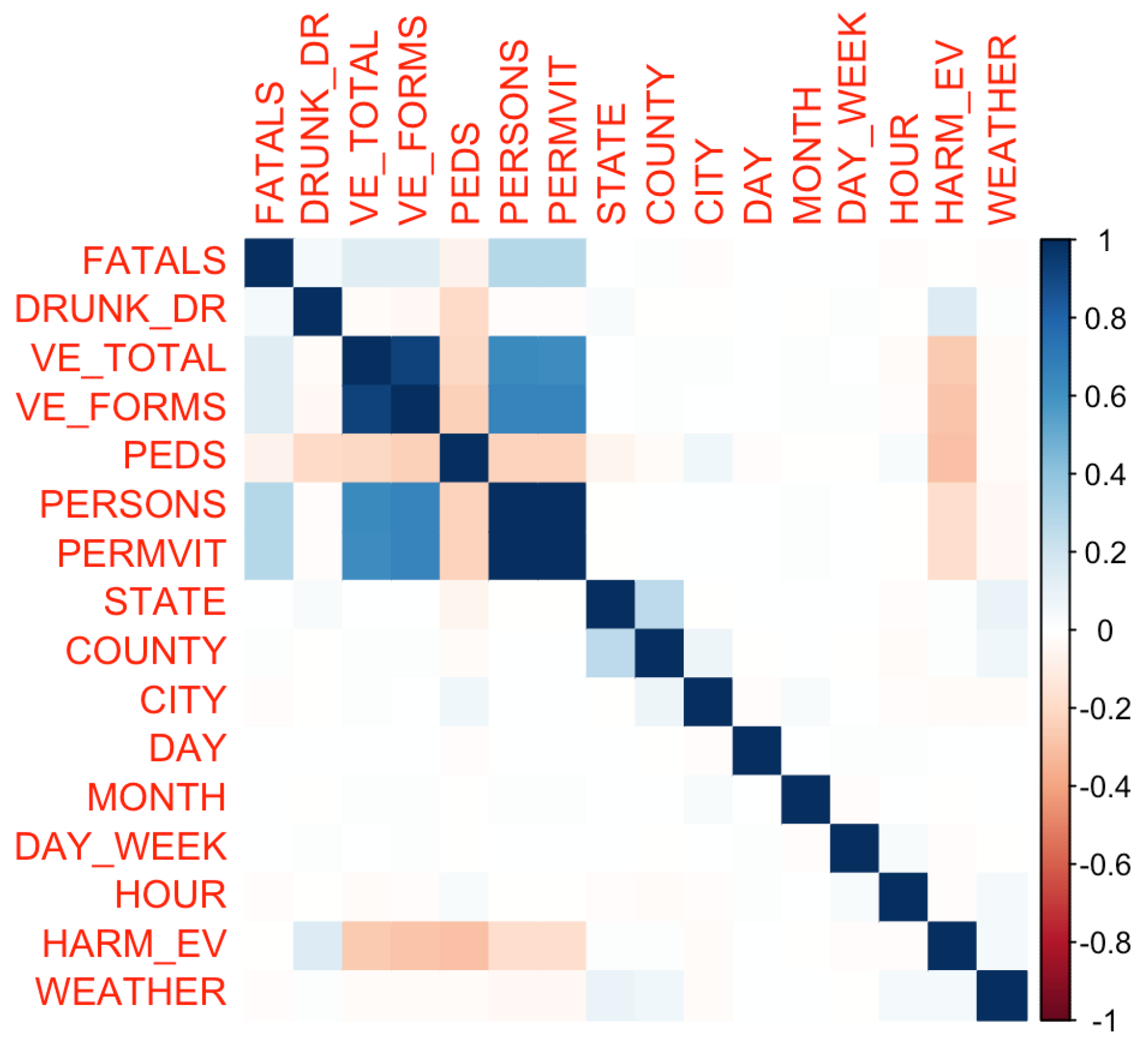
- Correlation Analysis: A correlation matrix was created to understand the relationships between numerical attributes, highlighting any potential interdependencies or redundancies.
- Summary of Accident Data Analysis Results
- -
- Preliminary Analysis: The dataset includes various attributes, such as information on the number of vehicles involved, alcohol influence, weather conditions, and the time of occurrence. Missing values in some columns were addressed during the analysis.
- -
- Key Data
- *
- On average, there are approximately 1.085 fatalities per accident, with a maximum of 8 fatalities in a single accident.
- *
- Approximately 26.6% of accidents involve a drunk driver.
- *
- Most accidents involve between one and two vehicles, and about 23% of accidents involve pedestrians.
- *
- Accidents are distributed throughout the day, with peaks in the afternoon and evening.
- -
- Correlation Analysis: VE_TOTAL and VE_FORMS are highly correlated. Accidents involving pedestrians (PEDS) tend to have fewer vehicles and persons.
- -
- Temporal Information: Accidents primarily occur in the afternoon and evening, with noticeable increases on certain weekdays.
- Head Size: The size of each head in the multi-head attention mechanism is set to 256.
- Number of Heads: We employ four attention heads, allowing the model to focus on different parts of the input simultaneously.
- Feed-forward Dimension: The dimensionality of the feed-forward network’s inner layer is set to 4.
- Number of Transformer Blocks: Our model is equipped with four Transformer blocks, each containing one multi-head attention layer and one feed-forward layer.
- MLP Units: After the Transformer blocks, the sequence is pooled globally and then passed through a feed-forward network with 128 units.
- Dropout: Dropout layers with rates of 0.4 (for the MLP) and 0.25 (for the Transformer encoder) are integrated to mitigate overfitting.
3. Evaluation
3.1. Detailed Exploration of Top Feature Weights
Implications of Top Feature Weights
- Trafficway Context: Features related to the type and classification of the trafficway, such as non-state inventoried roadways, played a significant role in accident occurrences. This indicates the importance of infrastructural factors in determining accident risk.
- Light and Environmental Conditions: Variables related to lighting (e.g., dawn or dusk) and weather conditions (e.g., cloudy) were paramount, suggesting that visibility and environmental factors substantially influence the likelihood of accidents.
- Temporal Factors: Features related to specific times, such as early mornings or specific days in a month, were notable, emphasizing the periodic nature of accident risks.
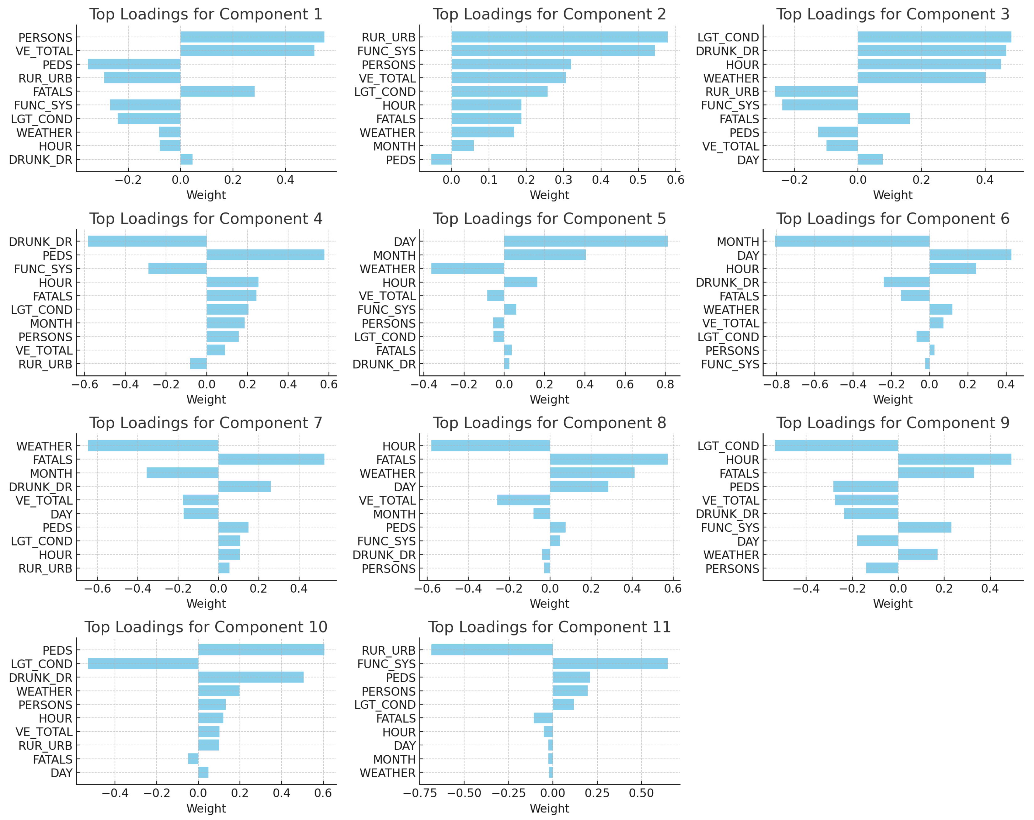
3.2. Interpretation of PCA Loading Results
3.3. Implications of the Findings
4. The Interplay of Forecasting, PCA, and Large Language Models in Autonomous Driving
4.1. Formalizing Accident Prediction for Autonomous Driving
4.2. Incorporating Principal Component Analysis
4.3. Leveraging Large Language Models in Autonomous Driving
4.4. Real-Time Intervention for Safer Autonomous Driving
4.5. Zephyr-7b- in Autonomous Driving: Pioneering Real-Time Interventions
4.6. Utilizing Language Models for Traffic Forecasting and Analysis
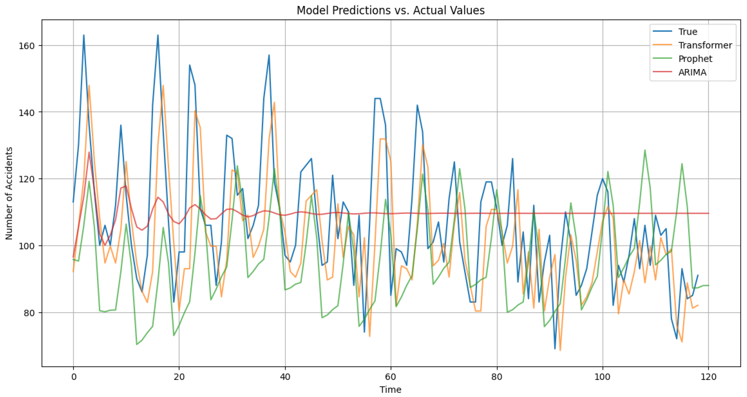
OpenAI GPT-4, LLaMA-2, and Zephyr-7b- in Traffic Forecasting
5. LLaVA: A Pioneer in Multi-Modal Understanding for Image Road Analysis
5.1. LLaVA-13b for Image Road Analysis
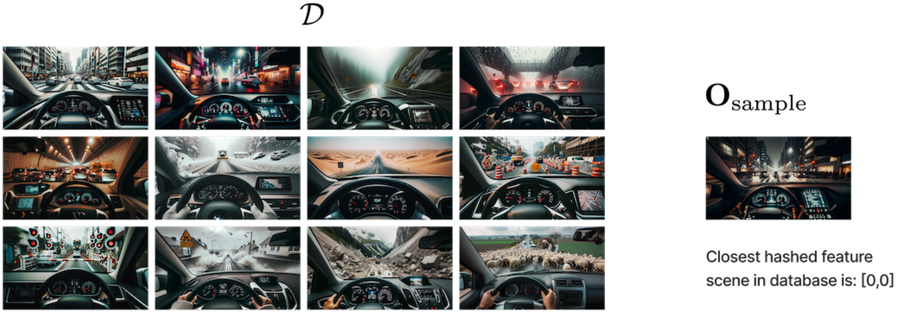
5.2. Image Hashing and Retrieval with DL Features for Enhanced Multimodal Descriptions
5.3. Bayesian Image Feature Extraction and Uncertainty Analysis
5.3.1. Bayesian Adaptation of ResNet
5.3.2. Feature Extraction and Image Hashing
5.3.3. Uncertainty Analysis
- Insights into dimensions bearing both maximal and minimal confidence.
- Potential triggers for precautionary measures in applications demanding high reliability, facilitating a more transparent and robust system.
- Mean features: This is the average value of the deep features for the sample after passing it through the Bayesian model multiple times. The deep features give a high-level, abstract representation of the image, and the mean provides the “central” or “most likely” representation in the presence of uncertainties in the model.
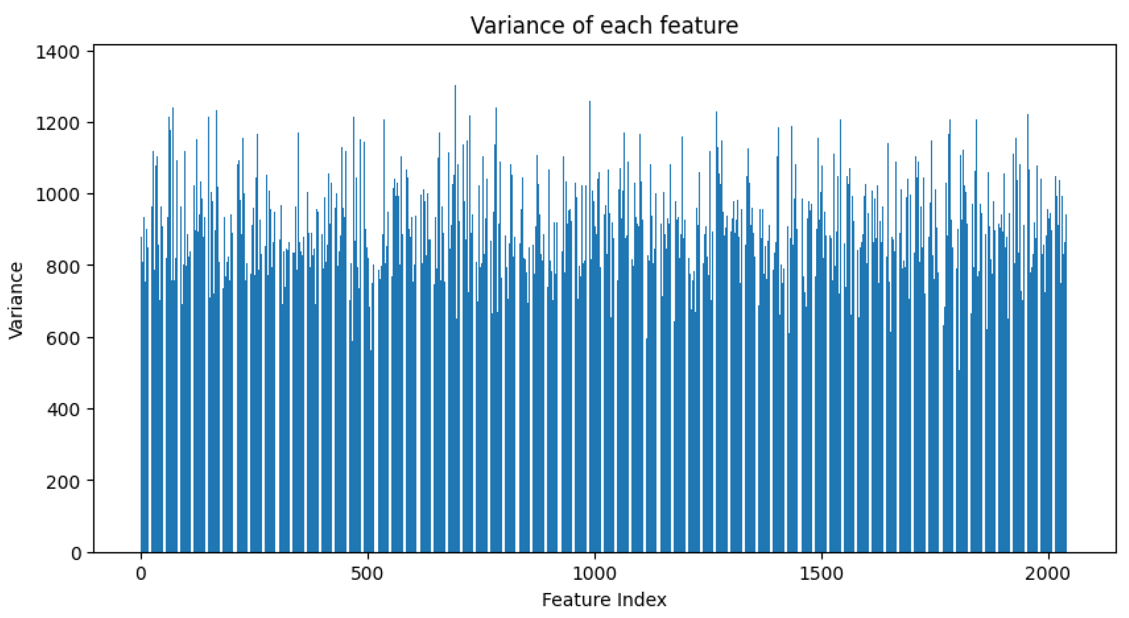
- Variance in features (see Figure 9): This captures the uncertainty or variability in the deep features for the sample under study after multiple forward passes through the Bayesian model. Higher values of variance for certain feature dimensions indicate higher uncertainties in those dimensions. This could arise from various factors like the inherent noise in the image, ambiguities in the scene, or uncertainties in the model parameters.
6. Discussion
7. Conclusions
Author Contributions
Funding
Institutional Review Board Statement
Informed Consent Statement
Data Availability Statement
Conflicts of Interest
Abbreviations
| Large Language Models | LLMs |
| Visual Language Models | VLMs |
| Principal Component Analysis | PCA |
| Generative Pre-Trained Transformers 4 with Vision | GPT-4V |
| Deep Learning | DL |
| Machine Learning | ML |
| Artificial Intelligence | AI |
| Large Language Model Meta AI | LLaMA |
| Large Language and Vision Assistant | LLaVA |
| AutoRegressive Integrated Moving Average | ARIMA |
References
- Guo, Y.; Tang, Z.; Guo, J. Could a Smart City Ameliorate Urban Traffic Congestion? A Quasi-Natural Experiment Based on a Smart City Pilot Program in China. Sustainability 2020, 12, 2291. [Google Scholar] [CrossRef]
- Zonouzi, M.N.; Kargari, M. Modeling uncertainties based on data mining approach in emergency service resource allocation. Comput. Ind. Eng. 2020, 145, 106485. [Google Scholar] [CrossRef]
- Vlahogianni, E.I.; Karlaftis, M.G.; Golias, J.C. Short-term traffic forecasting: Where we are and where we’re going. Transp. Res. Part Emerg. Technol. 2014, 43, 3–19. [Google Scholar] [CrossRef]
- Weng, W.; Fan, J.; Wu, H.; Hu, Y.; Tian, H.; Zhu, F.; Wu, J. A Decomposition Dynamic graph convolutional recurrent network for traffic forecasting. Pattern Recognit. 2023, 142, 109670. [Google Scholar] [CrossRef]
- Negash, N.M.; Yang, J. Driver Behavior Modeling Towards Autonomous Vehicles: Comprehensive Review. IEEE Access 2023, 11, 22788–22821. [Google Scholar] [CrossRef]
- Jiang, W.; Luo, J. Graph neural network for traffic forecasting: A survey. Expert Syst. Appl. 2022, 207, 117921. [Google Scholar] [CrossRef]
- Jiang, W.; Luo, J.; He, M.; Gu, W. Graph Neural Network for Traffic Forecasting: The Research Progress. ISPRS Int. J. Geo-Inf. 2023, 12, 100. [Google Scholar] [CrossRef]
- Li, G.; Zhong, S.; Deng, X.; Xiang, L.; Gary Chan, S.-H.; Li, R.; Liu, Y.; Zhang, M.; Hung, C.-C.; Peng, W.-C. A Lightweight and Accurate Spatial-Temporal Transformer for Traffic Forecasting. IEEE Trans. Knowl. Data Eng. 2022, 35, 10967–10980. [Google Scholar] [CrossRef]
- Guo, X.-Y.; Zhang, G.; Jia, A.-F. Study on mixed traffic of autonomous vehicles and human-driven vehicles with different cyber interaction approaches. Veh. Commun. 2023, 39, 100550. [Google Scholar] [CrossRef]
- Li, G.; Zhao, Z.; Guo, X.; Tang, L.; Zhang, H.; Wang, J. Towards integrated and fine-grained traffic forecasting: A spatio-temporal heterogeneous graph transformer approach. Inf. Fusion 2023, 102, 102063. [Google Scholar] [CrossRef]
- Chen, H.; Wang, T.; Chen, T.; Deng, W. Hyperspectral image classification based on fusing S3-PCA, 2D-SSA and random patch network. Remote Sens. 2023, 15, 3402. [Google Scholar] [CrossRef]
- Pham, H.; Dai, Z.; Ghiasi, G.; Kawaguchi, K.; Liu, H.; Yu, A.W.; Yu, J.; Chen, Y.; Luong, M.; Wu, Y.; et al. Combined scaling for open-vocabulary image classification. arXiv 2021, arXiv:2111.10050. [Google Scholar]
- Peng, B.; Li, C.; He, P.; Galley, M.; Gao, J. Instruction tuning with GPT-4. arXiv 2023, arXiv:2304.03277. [Google Scholar]
- Li, J.; Li, D.; Savarese, S.; Hoi, S. Blip-2: Bootstrapping language-image pre-training with frozen image encoders and large language models. arXiv 2023, arXiv:2301.12597. [Google Scholar]
- Ouyang, L.; Wu, J.; Jiang, X.; Almeida, D.; Wainwright, C.; Mishkin, P.; Zhang, C.; Agarwal, S.; Slama, K.; Ray, A.; et al. Training language models to follow instructions with human feedback. Adv. Neural Inf. Process. Syst. 2022, 35, 27730–27744. [Google Scholar]
- Minderer, M.; Gritsenko, A.; Austin, N.M.; Weissenborn, D.; Dosovitskiy, A.; Mahendran, A.; Arnab, A.; Dehghani, M.; Shen, Z.; Wang, X.; et al. Simple Open-Vocabulary Object Detection with Vision Transformers. arXiv 2022, arXiv:2205.06230. [Google Scholar]
- Minderer, M.; Gritsenko, A.; Houlsby, N. Scaling Open-Vocabulary Object Detection. arXiv 2023, arXiv:2306.09683. [Google Scholar]
- Bingham, E.; Chen, J.P.; Jankowiak, M.; Obermeyer, F.; Pradhan, N.; Karaletsos, T.; Singh, R.; Szerlip, P.; Horsfall, P.; Goodman, N.D. Pyro: Deep Universal Probabilistic Programming. J. Mach. Learn. Res. 2018, 20, 1–6. [Google Scholar]
- Ahangar, M.N.; Ahmed, Q.Z.; Khan, F.A.; Hafeez, M. A survey of autonomous vehicles: Enabling communication technologies and challenges. Sensors 2021, 21, 706. [Google Scholar] [CrossRef]
- Caesar, H.; Bankiti, V.; Lang, A.H.; Vora, S.; Liong, V.E.; Xu, Q.; Krishnan, A.; Pan, Y.; Baldan, G.; Beijbom, O. Nuscenes: A multimodal dataset for autonomous driving. In Proceedings of the IEEE/CVF Conference on Computer Vision and Pattern Recognition, New Orleans, LA, USA, 18–24 June2020; pp. 11621–11631. [Google Scholar]
- Yeong, D.J.; Velasco-Hernandez, G.; Barry, J.; Walsh, J. Sensor and sensor fusion technology in autonomous vehicles: A review. Sensors 2021, 21, 2140. [Google Scholar] [CrossRef]
- Hu, Y.; Yang, J.; Chen, L.; Li, K.; Sima, C.; Zhu, X.; Chai, S.; Du, S.; Lin, T.; Wang, W.; et al. Planning-oriented autonomous driving. In Proceedings of the IEEE/CVF Conference on Computer Vision and Pattern Recognition, Vancouver, BC, Canada, 18–22 June 2023; pp. 17853–17862. [Google Scholar]
- Mao, J.; Qian, Y.; Zhao, H.; Wang, Y. GPT-Driver: Learning to Drive with GPT. arXiv 2023, arXiv:2310.01415. [Google Scholar]
- Vaswani, A.; Shazeer, N.; Parmar, N.; Uszkoreit, J.; Jones, L.; Gomez, A.N.; Kaiser, Ł.; Polosukhin, I. Attention is all you need. In Proceedings of the Advances in Neural Information Processing Systems 30 (NIPS 2017), Long Beach, CA, USA, 4–9 December 2017; pp. 5998–6008. [Google Scholar]
- Shumway, R.H.; Stoffer, D.S. ARIMA models. In Time Series Analysis and Its Applications: With R Examples; Springer: Cham, Switzerland, 2017; pp. 75–163. [Google Scholar] [CrossRef]
- Taylor, S.J.; Letham, B. Forecasting at Scale. Am. Stat. 2018, 72, 37–45. [Google Scholar] [CrossRef]
- Miao, Y.; Bai, X.; Cao, Y.; Liu, Y.; Dai, F.; Wang, F.; Qi, L.; Dou, W. A Novel Short-Term Traffic Prediction Model based on SVD and ARIMA with Blockchain in Industrial Internet of Things. IEEE Internet Things J. 2023. [Google Scholar] [CrossRef]
- Zaman, M.; Saha, S.; Abdelwahed, S. Assessing the Suitability of Different Machine Learning Approaches for Smart Traffic Mobility. In Proceedings of the 2023 IEEE Transportation Electrification Conference & Expo (ITEC), Detroit, MI, USA, 21–23 June 2023; IEEE: Piscataway, NJ, USA, 2023; pp. 1–6. [Google Scholar]
- Nguyen, N.-L.; Vo, H.-T.; Lam, G.-H.; Nguyen, T.-B.; Do, T.-H. Real-Time Traffic Congestion Forecasting Using Prophet and Spark Streaming. In International Conference on Intelligence of Things; Springer International Publishing: Cham, Switzerland, 2022; pp. 388–397. [Google Scholar]
- Chen, C.; Liu, Y.; Chen, L.; Zhang, C. Bidirectional spatial-temporal adaptive transformer for Urban traffic flow forecasting. IEEE Trans. Neural Net. Learn. Syst. 2022, 34, 6913–6925. [Google Scholar] [CrossRef]
- Rob, J. Hyndman and George Athanasopoulos. In Forecasting: Principles and Practice; OTexts, 2018; Available online: https://otexts.com/fpp2/ (accessed on 1 October 2023).
- Radford, A.; Kim, J.W.; Hallacy, C.; Ramesh, A.; Goh, G.; Agarwal, S.; Sastry, G.; Askell, A.; Mishkin, P.; Clark, J.; et al. Learning transferable visual models from natural language supervision. In Proceedings of the 38th International Conference on Machine Learning, Virtual, 18–24 July 2021. [Google Scholar]
- Wang, Y.; Kordi, Y.; Mishra, S.; Liu, A.; Smith, N.A.; Khashabi, D.; Hajishirzi, H. Self-instruct: Aligning language model with self generated instructions. arXiv 2022, arXiv:2212.10560. [Google Scholar]
- Jiang, A.Q.; Sablayrolles, A.; Mensch, A.; Bamford, C.; Chaplot, D.S.; Casas, D.d.; Bressand, F.; Lengyel, G.; Lample, G.; Saulnier, L.; et al. Mistral 7B. arXiv 2023, arXiv:2310.06825. [Google Scholar]
- Rafailov, R.; Sharma, A.; Mitchell, E.; Ermon, S.; Manning, C.D.; Finn, C. Direct Preference Optimization: Your Language Model is Secretly a Reward Model. arXiv 2023, arXiv:2305.18290. [Google Scholar]
- Taori, R.; Gulrajani, I.; Zhang, T.; Dubois, Y.; Li, X.; Guestrin, C.; Liang, P.; Hashimoto, T.B. Stanford Alpaca: An Instruction-Following Llama Model. 2023. Available online: https://github.com/tatsu-lab/stanford_alpaca (accessed on 1 October 2023).
- Touvron, H.; Lavril, T.; Izacard, G.; Martinet, X.; Lachaux, M.; Lacroix, T.; Rozière, B.; Goyal, N.; Hambro, E.; Azhar, F.; et al. Llama: Open and efficient foundation language models. arXiv 2023, arXiv:2302.13971. [Google Scholar]
- Liu, H.; Li, C.; Wu, Q.; Lee, Y.J. Visual instruction tuning. In Proceedings of the NeurIPS 2023, New Orleans, LA, USA, 10–16 December 2023. [Google Scholar]
- Xia, X.; Dong, G.; Li, F.; Zhu, L.; Ying, X. When CLIP meets cross-modal hashing retrieval: A new strong baseline. Inf. Fusion 2023, 100, 101968. [Google Scholar]
- Phan, D.; Pradhan, N.; Jankowiak, M. Composable Effects for Flexible and Accelerated Probabilistic Programming in NumPyro. arXiv 2019, arXiv:1912.11554. [Google Scholar]
- Ramesh, A.; Pavlov, M.; Goh, G.; Gray, S.; Voss, C.; Radford, A.; Chen, M.; Sutskever, I. Zero-Shot Text-to-Image Generation. In Proceedings of the 38th International Conference on Machine Learning, Virtual, 18–24 July 2021; Volume 139, pp. 8821–8831. [Google Scholar]


| Component | Loadings |
|---|---|
| Component 1 | FUNC_SYS_96: Trafficway Not in State Inventory, RUR_URB_6: Trafficway Not in State Inventory, LGT_COND_5: Dusk, DAY_15: Day of Crash—The accident occurred on the 15th day of the month, HOUR_20: Hour of Crash—The accident occurred at 8 p.m., MONTH_8: Month of Crash—The accident occurred in August, WEATHER_10: Cloudy, PEDS_1: Number of Persons Not in Motor Vehicles—one person, LGT_COND_9: Reported as Unknown, DRUNK_DR_1: Number of Drinking Drivers Involved in the Fatal Crash—one driver. |
| Component 2 | VE_TOTAL_2: Number of Vehicles in Crash—two vehicles, PERSONS_5: Number of Person Forms—five persons, LGT_COND_3: Dark but Lighted, FATALS_4: Number of Fatalities That Occurred in the Crash—four fatalities, PERSONS_2: Number of Person Forms—two persons, WEATHER_5: Fog, Smog, Smoke, PEDS_1: Number of Persons Not in Motor Vehicles—one person, DAY_5: Day of Crash—The accident occurred on the fifth day of the month, RUR_URB_9: Land Use—Unknown, FUNC_SYS_99: Functional System—Unknown. |
| Component 3 | FUNC_SYS_99: Functional System—Unknown, RUR_URB_9: Land Use—Unknown, FATALS_4: Number of Fatalities That Occurred in the Crash—four fatalities, DAY_28: Day of Crash—The accident occurred on the 28th day of the month, HOUR_9: Hour of Crash—The accident occurred at 9 a.m., WEATHER_5: Fog, Smog, Smoke, HOUR_2: Hour of Crash—The accident occurred at 2 a.m., DAY_5: Day of Crash—The accident occurred on the fifth day of the month, DAY_4: Day of Crash—The accident occurred on the fourth day of the month, HOUR_17: Hour of Crash—The accident occurred at 5 p.m. |
| Component 4 | LGT_COND_3: Dark but Lighted, HOUR_7: Hour of Crash—The accident occurred at 7 a.m., DAY_31: Day of Crash—The accident occurred on the 31st day of the month, RUR_URB_9: Land Use—Unknown, HOUR_23: Hour of Crash—The accident occurred at 11 p.m., HOUR_0: Hour of Crash—The accident occurred at 12 a.m., WEATHER_5: Fog, Smog, Smoke, MONTH_2: Month of Crash—The accident occurred in February, LGT_COND_2: Dark—Not Lighted, DAY_6: Day of Crash—The accident occurred on the sixth day of the month. |
| Component 5 | HOUR_17: Hour of Crash—The accident occurred at 5 p.m., LGT_COND_2: Dark—Not Lighted, HOUR_18: Hour of Crash—The accident occurred at 6 p.m., PERSONS_2: Number of Person Forms—two persons, VE_TOTAL_2: Number of Vehicles in Crash—two vehicles, HOUR_3: Hour of Crash—The accident occurred at 3 a.m., HOUR_6: Hour of Crash—The accident occurred at 6 a.m., DAY_14: Day of Crash—The accident occurred on the 14th day of the month, FATALS_2: Number of Fatalities That Occurred in the Crash—two fatalities, PERSONS_1: Number of Person Forms—one person. |
| Component 6 | HOUR_6: Hour of Crash—The accident occurred at 6 a.m., LGT_COND_2: Dark—Not Lighted, HOUR_7: Hour of Crash—The accident occurred at 7 a.m., RUR_URB_9: Land Use—Unknown, LGT_COND_5: Dusk, HOUR_5: Hour of Crash—The accident occurred at 5 a.m., LGT_COND_3: Dark but Lighted, PERSONS_2: Number of Person Forms—two persons, VE_TOTAL_2: Number of Vehicles in Crash—two vehicles, DAY_30: Day of Crash—The accident occurred on the 30th day of the month. |
| Component | Loadings |
|---|---|
| Component 7 | LGT_COND_3: Dark but Lighted, LGT_COND_2: Dark—Not Lighted, LGT_COND_5: Dusk, HOUR_0: Hour of Crash—The accident occurred at 12 a.m., HOUR_7: Hour of Crash—The accident occurred at 7 a.m., HOUR_23: Hour of Crash—The accident occurred at 11 p.m., DAY_1: Day of Crash—The accident occurred on the first day of the month, DAY_2: Day of Crash—The accident occurred on the second day of the month, RUR_URB_9: Land Use—Unknown, DAY_3: Day of Crash—The accident occurred on the third day of the month. |
| Component 8 | HOUR_7: Hour of Crash—The accident occurred at 7 a.m., HOUR_6: Hour of Crash—The accident occurred at 6 a.m., LGT_COND_2: Dark—Not Lighted, LGT_COND_3: Dark but Lighted, HOUR_8: Hour of Crash—The accident occurred at 8 a.m., DAY_1: Day of Crash—The accident occurred on the first day of the month, DAY_2: Day of Crash—The accident occurred on the second day of the month, PERSONS_2: Number of Person Forms—two persons, VE_TOTAL_2: Number of Vehicles in Crash—two vehicles, LGT_COND_5: Dusk. |
| Component 9 | LGT_COND_3: Dark but Lighted, LGT_COND_2: Dark—Not Lighted, RUR_URB_9: Land Use—Unknown, HOUR_6: Hour of Crash—The accident occurred at 6 a.m., HOUR_7: Hour of Crash—The accident occurred at 7 a.m., DAY_1: Day of Crash—The accident occurred on the first day of the month, LGT_COND_5: Dusk, HOUR_8: Hour of Crash—The accident occurred at 8 a.m., HOUR_5: Hour of Crash—The accident occurred at 5 a.m., PERSONS_2: Number of Person Forms—two persons. |
| Component 10 | HOUR_8: Hour of Crash—The accident occurred at 8 a.m., LGT_COND_2: Dark—Not Lighted, LGT_COND_3: Dark but Lighted, HOUR_7: Hour of Crash—The accident occurred at 7 a.m., RUR_URB_9: Land Use—Unknown, HOUR_6: Hour of Crash—The accident occurred at 6 a.m., DAY_1: Day of Crash—The accident occurred on the first day of the month, LGT_COND_5: Dusk, PERSONS_2: Number of Person Forms—two persons, VE_TOTAL_2: Number of Vehicles in Crash—two vehicles. |
| Component 11 | LGT_COND_2: Dark—Not Lighted, LGT_COND_3: Dark but Lighted, HOUR_8: Hour of Crash—The accident occurred at 8 a.m., HOUR_7: Hour of Crash—The accident occurred at 7 a.m., RUR_URB_9: Land Use—Unknown, DAY_1: Day of Crash—The accident occurred on the first day of the month, HOUR_6: Hour of Crash—The accident occurred at 6 a.m., PERSONS_2: Number of Person Forms—two persons, VE_TOTAL_2: Number of Vehicles in Crash—two vehicles, LGT_COND_5: Dusk. |
| Component | Primary Influences |
|---|---|
| Component 1 | This component is strongly influenced by variables such as the functional system of the roadway (with a specific emphasis on trafficways not in the state inventory), the land use context indicating trafficways not in the state inventory, light conditions during the accident (specifically, unknown lighting conditions), and the presence of alcohol in drivers. |
| Component 2 | The second component focuses on the total number of vehicles involved in the crash, the number of persons involved, light conditions at dawn, the number of fatalities, and the type of weather conditions (cloudy). |
| Component 3 | This component is influenced by the functional system of the roadway (unknown category), land use context indicating unknown urbanization, the number of fatalities, and specific days and hours during which the accident occurred. |
| Component 4 | The fourth component places emphasis on the light conditions during the accident (specifically, unknown lighting conditions), rural or urban context of the accident site, and the functional system of the roadway. |
| Component 5 | This component is influenced by the month of the accident, the number of persons involved, and the land use context, specifically differentiating between urban and rural environments. |
| Component 6 | The sixth component seems to be influenced mainly by the total number of vehicles involved in the crash, the functional system of the roadway (especially interstate roads), and the number of persons involved in the accident. |
| Component 7 | This component is influenced by the functional system of the roadway, the number of vehicles involved in the crash, and the specific days and hours during which the accident occurred. |
| Component 8 | The eighth component emphasizes the functional system of the roadway, the number of persons not in motor vehicles, and specific weather conditions during the accident. |
| Component 9 | This component focuses on the number of persons involved in the accident, specific days during which the accident occurred, and the functional system of the roadway. |
| Component 10 | The tenth component places emphasis on the functional system of the roadway, specific days during which the accident occurred, and the hour of the crash. |
| Component 11 | This component seems to be influenced mainly by the number of persons not in motor vehicles during the accident, the land use context indicating the urbanization of the accident site, and the functional system of the roadway. |
| Sample | Prompt: Analyze the Road Conditions, Potential Obstacles, and Safety Concerns Visible in This Image. |
|---|---|
 | In the image, we see a busy city street with a large number of cars and pedestrians. The road is filled with traffic, including cars, trucks, and even a bus. There are multiple traffic lights along the street, which helps manage the flow of vehicles and pedestrians. The potential obstacles and safety concerns visible in the image include the high volume of traffic, which can lead to congestion and increased risk of accidents. The presence of pedestrians crossing the street also adds to the complexity of the scene, as drivers must be vigilant and cautious to avoid collisions. Additionally, the image shows a car driving through an intersection, which is a common area for accidents to occur. Drivers must pay close attention to the traffic lights and other vehicles to ensure safe navigation through the intersection. Overall, the image depicts a bustling city street with various obstacles and safety concerns that require drivers and pedestrians to be attentive and cautious to maintain safety and order. |
 | In the image, the road appears to be wet, which can lead to reduced visibility and potentially slippery driving conditions. The car’s headlights are on, indicating that the driver is trying to improve visibility in the foggy and wet conditions. However, the foggy conditions can still make it challenging for the driver to see clearly and anticipate potential obstacles. There are several traffic signs visible along the road, which are essential for providing guidance and information to drivers. The presence of these signs indicates that the road is well-maintained and organized, reducing the risk of accidents. The image also shows a car driving down the road, which could be a potential obstacle for other vehicles. Drivers should be cautious and maintain a safe distance from other vehicles to avoid collisions in such conditions. Overall, the image highlights the importance of being vigilant and cautious while driving in wet and foggy conditions, as visibility is reduced, and the risk of accidents can increase. |
| Sample | Prompt: Provide a Real-Time Analysis of the Road Conditions, Potential Obstacles, and Safety Concerns Visible in This Image. Update on Any Changes or Movements That Might Affect Driving Decisions. |
|---|---|
 | In the image, a car is driving down a wet highway with heavy rain. The road appears to be wet, which can lead to reduced visibility and increased braking distance. The driver should exercise caution and maintain a safe distance from other vehicles. There are several cars on the road, including a truck, which indicates that the traffic is moderate. The driver should be aware of other vehicles’ movements and adjust their speed accordingly to avoid collisions. Additionally, the presence of traffic lights suggests that the driver should pay attention to the signals and follow the rules of the road. Overall, the driver should remain vigilant and cautious while driving in these conditions, as the wet road and heavy rain can pose challenges to safe driving. |
 | In the image, a car is driving down a road near a beach, with a surreal scene of a wave crashing into the beach and a flock of birds flying overhead. The road appears to be wet, which could indicate recent rain or a nearby water source. The presence of birds flying close to the road could pose a potential hazard for the driver, as they might suddenly land on the road or distract the driver. The surreal wave crashing into the beach suggests that the area might be prone to flooding or other natural disasters, which could impact driving conditions and safety. The driver should remain vigilant and cautious while navigating the road, taking into account the wet road conditions, potential bird hazards, and the possibility of natural disasters. |
| Method | Application | Advantages | Disadvantages | Limits in Practice |
|---|---|---|---|---|
| DL | Time series forecasting of traffic data | High accuracy, captures complex patterns | Requires large amounts of data, computationally expensive | May not perform well with sparse or noisy data |
| PCA | Dimensionality reduction for traffic data | Reduces data complexity, helps identify major patterns | Loss of information, assumes linear relationships | Not suitable for non-linear patterns |
| LLMs | Interpreting PCA loadings, real-time traffic forecasting, real-time risk assessment | High interpretability, versatile applications | Requires large computational resources, may generate biased outputs | May not always provide accurate real-time responses |
| LLaVA-13b, GPT-4V | Detailed image road analysis | High accuracy, provides context-aware insights | Computationally expensive, requires large amounts of data | May struggle with ambiguous or novel scenarios |
| Bayesian image feature extraction | Deep feature extraction with uncertainty analysis | Provides uncertainty estimates, enhances robustness | Computationally expensive, requires understanding of Bayesian methods | May be overkill for simple applications |
| Real-time intervention | Dynamic adjustment of driving style based on risk assessment | Enhances vehicle safety, adaptable to changing conditions | Depends on accurate risk assessment, may require frequent updates | May not cover all potential road scenarios |
Disclaimer/Publisher’s Note: The statements, opinions and data contained in all publications are solely those of the individual author(s) and contributor(s) and not of MDPI and/or the editor(s). MDPI and/or the editor(s) disclaim responsibility for any injury to people or property resulting from any ideas, methods, instructions or products referred to in the content. |
© 2023 by the authors. Licensee MDPI, Basel, Switzerland. This article is an open access article distributed under the terms and conditions of the Creative Commons Attribution (CC BY) license (https://creativecommons.org/licenses/by/4.0/).
Share and Cite
de Zarzà, I.; de Curtò, J.; Roig, G.; Calafate, C.T. LLM Multimodal Traffic Accident Forecasting. Sensors 2023, 23, 9225. https://doi.org/10.3390/s23229225
de Zarzà I, de Curtò J, Roig G, Calafate CT. LLM Multimodal Traffic Accident Forecasting. Sensors. 2023; 23(22):9225. https://doi.org/10.3390/s23229225
Chicago/Turabian Stylede Zarzà, I., J. de Curtò, Gemma Roig, and Carlos T. Calafate. 2023. "LLM Multimodal Traffic Accident Forecasting" Sensors 23, no. 22: 9225. https://doi.org/10.3390/s23229225
APA Stylede Zarzà, I., de Curtò, J., Roig, G., & Calafate, C. T. (2023). LLM Multimodal Traffic Accident Forecasting. Sensors, 23(22), 9225. https://doi.org/10.3390/s23229225