Radial Thermoelectric Model for Stranded Transmission Line Conductors

Abstract

Bare-stranded conductors play a critical role in the efficiency and safe operation of transmission lines. The heat generated in the interior of the conductor is conducted radially to the outer surface, creating a radial thermal gradient. The radial temperature gradient between the core and the surface depends on multiple factors, such as stranding, number of layers, current level, electrical resistance and the effective radial thermal conductivity. Therefore, the radial temperature model must be considered when developing accurate conductor models. Such models are particularly important in the development of dynamic line rating (DLR) approaches to allow the full current carrying capacity of the conductor to be utilized while ensuring safe operation. This paper develops a radial one-dimensional thermoelectric model for bare-stranded conductors used in transmission lines. The accuracy of the proposed model is determined by experimental tests performed on three conductors.

1. Introduction

Global demand for electricity has been growing steadily, and projections indicate that this trend will continue. According to projections by the International Energy Agency (IEA), the share of electricity in final energy consumption is expected to increase from 20% today to more than 50% by 2050 [1]. The efficiency, reliability and availability of power lines will become increasingly important as electrification continues [2], so operators need reliable methods to operate overhead transmission lines at maximum capacity [3] without compromising their safety. Conductor sag is a key parameter for the safe operation of overhead transmission lines [4], as it determines the ground clearance. By limiting the maximum operating conductor temperature, sag, ground clearance [2,5] and conductor integrity [6] can be maintained at safe levels. Transmission lines occasionally operate at maximum design ratings [7]. Due to various factors, the construction of new transmission lines is very problematic today, so other options to increase the capacity of existing power lines are being analyzed, such as replacing existing aluminum conductors steel reinforced (ACSRs) with high-temperature low-sag (HTLS) conductors or by applying dynamic line rating (DLR) strategies. Unlike static line rating (SLR), which applies conservative ratings based on the worst-case weather conditions (emissivity = 0.8, high annual ambient temperature, wind speed of 0.5 m/s and solar irradiance of 1000 W/m² [7]), DLR is based on real-time weather ratings [8,9,10]. By considering actual values of the solar irradiance, wind speed and direction and ambient temperature, combined with the application of DLR line models, a more realistic line rating can be determined [11,12], allowing the full capacity of the line to be utilized [13].

DLR approaches require the measurement of several variables, including conductor current and temperature and weather-related variables, such as ambient temperature, solar irradiance and wind speed and direction [14,15]. Next, the conductor heat balance equation is solved using methods such as those presented in Cigré [11], IEEE [12] or IEC [16], which also require knowledge of all conductor dimensions and material properties of the conductors. By solving the dynamic transient heat equation, it is possible to determine the maximum conductor rating. The DLR must ensure the stability of the transmission line at high operating currents while respecting the maximum allowable temperature of the conductor to ensure that safe limits of sag and annealing effect on the aluminum material are not exceeded [17]. For this purpose, it is essential to have a detailed thermoelectric model of the conductor, capable of predicting not only the surface temperature but also the higher internal temperatures of the conductor.

However, most of the models published in the technical literature assume a homogeneous temperature distribution within the conductor [11,12,16], which is a simplification of reality. Although this assumption may be correct in many cases, it can lead to non-negligible deviations in others, e.g., when considering ACSR conductors with at least three aluminum layers and high current densities [18], so that differences between 10 °C and 25 °C [12] up to 30 °C [19] have been reported. Various authors have obtained formulas for determining the radial temperature distribution of power conductors [11,12,17,19,20]. However, they make different assumptions, such as steady-state operation or uniform radial electrical conductivity, and do not allow the development of a transient model by themselves. In addition, most of these references provide experimental results, but they lack the development of a transient model capable of determining the thermal behavior of the conductor, taking into account the radial temperature distribution.

The temperature of the conductor results from a thermal balance between the heating terms (Joule and solar heating) and the cooling terms (radiative and convective cooling). If the heating terms are greater than the cooling terms, the conductor heats up; otherwise, it cools down. In these cases, the difference between the heat input and the heat output is the stored power term (see Section 2 for more details). While the radiative and convective cooling terms depend on the surface temperature, the Joule heating and stored power terms depend on the internal or average temperature of the conductor. Therefore, existing models that assume a homogeneous temperature distribution lack this detailed analysis because they assume no difference between the surface temperature and the center temperature of the conductor.

Therefore, a transient thermoelectric radial model of bare-stranded conductors is required. This can be achieved by modifying the standard methods used for calculating the maximum current carrying capacity of a conductor described in the standards [11,12,16] to account for the higher core temperature of the conductor [17].

The novelties and contributions of this paper are as follows. First, it focuses on improving the thermoelectric transmission line conductor models described in the international standards [11,12,16] to consider the radial temperature distribution in order to have a more accurate picture of the temperature distribution within the conductor. Second, this paper proposes an accurate and fast one-dimensional thermoelectric conductor model that considers the radial temperature distribution and assumes that the heat flows radially from the center of the core to the outer surface. Third, results showing how the radial temperature distribution affects the conductor heating are also presented. Fourth, the paper also presents experimental results of three types of conductors, namely, an all-aluminum alloy conductor (AAAC), an aluminum conductor steel reinforced (ACSR), and an aluminum conductor composite core (ACCC), a type of high-temperature low-sag (HTLS) conductor. Experimental results allow the accuracy and usefulness of the radial model presented in this paper to be evaluated.

The remainder of the paper is organized as follows. Section 2 develops the transient heat transfer equations and their components. Section 3 details the proposed one-dimensional discretization of the problem to determine the radial temperature distribution within the conductor. Section 4 details the importance of effective radial thermal conductivity in the proposed model. Section 5 develops the equations to solve the proposed radial model. Section 6 describes the transmission line conductors analyzed and the experimental setup. Section 7 validates the proposed radial model from the experimental results. Finally, Section 8 concludes this paper.

2. Transient Heat Balance Equation

This section develops the different terms in the transient heat balance equation that describe the thermoelectric behavior of a bare conductor [11,12,21],

$$(P_{internal}+P_{solar})-(P_{conv}+P_{rad})=m{c}_p(T)\frac{dT}{dt}=P_{stored} [\mathrm{W}/\mathrm{m}]$$

(1)

where m (kg/m) is the conductor mass per unit length, c_p(T) (J/(kg °C)) is the specific heat capacity of the conductor material, T (°C) is the average temperature of the conductor, P_internal (W/m) is the term related to the internal power losses generated in the conductor per unit length, P_solar (W/m) is the solar heat gain per unit length, P_conv (W/m) is the convective cooling term per unit length and P_rad (W/m) is the radiative cooling per unit length. For a better understanding, the terms in (1) are shown in Figure 1.

According to (1), under thermal equilibrium, the total heat loss is equal to the total heat gain. Under transient conditions, where there is no thermal equilibrium, the difference between the total heat gain and the total heat loss is the neat heat stored in the conductor [11]. The various terms in (1) are developed in Section 2, but P_internal = i²(t)r_AC(T) (W/m) is the internal heating, where i(t) (A) is the RMS value of the current measured at time instant t (s) and r_AC (W/m) is the alternating current (AC) resistance per unit length of the conductor.

While the terms P_internal = i²(t)r_AC(T) and P_stored = mc_p(T)dT/dt depend on the average conductor temperature T, the terms P_conv and P_rad depend on the conductor surface temperature. Note that P_internal = i²(t)r_AC(T) is usually the main source of heating, and the AC resistance depends on the temperature distribution inside the conductor. In addition, effects such as creep, annealing and sag of the conductor are strongly affected by the radial temperature distribution within the conductor [22]. Therefore, accurate thermoelectric conductor models must take into account the temperature distribution within the conductor.

2.1. Stored Heat

Under transient conditions, i.e., without thermal equilibrium, the heat stored in the conductor per unit length can be expressed as,

$$P_{stored}=m{c}_p(T)\frac{dT}{dt} [\mathrm{W}/\mathrm{m}]$$

(2)

2.2. Internal Heating

ACSR conductors consist of an inner core of galvanized steel strands and several layers of aluminum strands wound helically around the steel strands [23]. While the core provides the mechanical strength [24], the aluminum strands carry most of the current [25]. Due to the specific configuration and the magnetic properties of the steel core, the ac magnetic flux causes eddy currents, hysteresis losses in the core and a redistribution of the currents in the aluminum layers [18,26], increasing the conductor’s AC resistance [24]. The internal losses P_internal can be determined as [8,21,27,28],

P_internal = P_Joule + P_mag + P_redis = i²(t)r_AC (W/m)

(3)

The internal losses have various components, namely the Joule losses (P_Joule), the core losses due to the hysteresis and eddy current effects (P_mag) and the redistribution losses (P_redis). According to (3), the internal losses are related to the AC resistance per unit length of the conductor r_AC (Ω/m) and the electric current i(t).

In the case of conductors without a magnetic core, this results in P_internal = P_Joule since P_mag = P_redis = 0.

The electrical resistivity ρ_e of the conductor changes with temperature according to,

ρ_e(T) = ρ_e,To [1 + α_AC(T − T₀)]

(4)

where T₀ is the reference temperature (usually 293.15 K), T (K) is the average temperature of the conductor temperature, and α_AC (K⁻¹) is the temperature coefficient of the resistivity under alternating current. The temperature dependence of the conductor resistance per unit length r_AC(T) follows a similar law,

r_AC(T) = r_AC,To [1 + α_AC(T − T₀)]

(5)

Since P_internal is by far the largest source of heat in power conductors [8,27], r_AC is an important parameter for building accurate thermoelectric models of conductors because it accounts for magnetic and eddy current effects. Note that r_AC can be calculated from r_DC (it is typically found in the manufacturers’ datasheets) using the procedure described in [11], or it can be measured directly as described in [28]. In this paper, r_AC is measured directly.

2.3. Natural Convective Heat Loss

According to IEEE Std. 738 [12], assuming a cylindrical conductor of outer diameter D_c (m), the natural convective heat loss per unit length can be calculated as follows,

P_conv = hπD_c(T_s − T_air) (W/m)

(6)

where T_s (K) and T_air (K) are the conductor surface temperature and air temperature, respectively, and h (W/(m²K)) is the heat transfer coefficient, which can be calculated under natural convection conditions (no wind, worst case) according to IEEE Std. 738 [12] as,

$$h=\frac{3.645}{\pi }{\rho }_{air}^{0.5}{D}_c^{-0.25}{(T_s-T_{air})}^{0.25}$$

(7)

Note that the air density ρ_air (kg/m³), which depends on the conductor height H (m), and the temperatures of the air and the outer surface of the conductor, T_air (K) and T_s (K), respectively, can be determined as [12],

ρ_air = (1.293 − 1.525 × 10⁻⁴H + 6.379 ×·10⁻⁹H²)/[1 + 1.835 ×·10⁻³(T_air + T_s)] (kg/m³)

(8)

2.4. Radiative Heat Loss

The radiative heat loss per unit length of the conductor can be calculated as [11],

P_rad = πεD_cσ_B[T_s⁴ − T_air⁴] (W/m)

(9)

where ε (-) is the dimensionless emissivity coefficient and σ_B = 5.67037 × 10⁻⁸ W/(m²K⁴) is the Stefan–Boltzmann constant. The effect of this term becomes very important at high conductor temperatures.

2.5. Solar Heat Gain

The solar heat gain P_solar (W/m) can be calculated as [11,16],

$$P_{solar}=\alpha Q_{sr}{D}_c (\mathrm{W}/\mathrm{m})$$

(10)

where α ∈ [0, 1] and is the absorptivity of the conductor and Q_sr (W/m²) is the total solar irradiance. This formulation is convenient because global radiation meters are now affordable, reliable and widely available. According to (10), the effect of solar heating increases with the conductor diameter [29]. Note that according to Kirchhoff’s law of thermal radiation, α ≈ ε. This equality also holds for non-equilibrium processes where radiative emission is produced exclusively by microscopic thermal transitions [30].

3. One-Dimensional Discretization of the Radial Temperature Distribution Problem

Although the conductors are made of aluminum strands with very good conductivity, they have a radial temperature distribution that cannot be neglected, especially when the conductors are operated at high temperatures. The terms P_internal and dT/dt in the heat balance Equation (1) depend on the average internal temperature of the conductor, while the terms P_conv and P_rad depend on the surface temperature. Since these two temperatures are different, it is necessary to know the radial temperature distribution of the conductor. To determine the radial temperature distribution, it is assumed that the heat flows radially from the center of the core to the outer surface. Due to the cylindrical geometry, a symmetric radial distribution can be assumed, allowing the problem to be discretized in one dimension, as shown in Figure 2.

The one-dimensional radial discretization shown in Figure 2 consists of j = 1, …, n = N_a + N_b + 1 nodes. It is assumed that the nodal temperatures of a generic node i can be determined from the nodal temperatures of the two adjacent nodes to the left and right sides. While the first node j = 1 is located in the center of the conductor (center of the core), the last node j = n is located in the periphery of the conductor (outer surface). The discretized form of the heat transfer problem expressed by (1) is solved through the radial axis as,

$$a_i^j{T}_{{}_{,}i-1}^{j+1}+b_i^j{T}_{{}_{,}i}^{j+1}+c_i^j{T}_{{}_{,}i+1}^{j+1}-d_i^j=0$$

(11)

where a_i^j, b_i^j, c_i^j and d_i^j are constant coefficients, i is the index related to the radial steps and j is the index related to the time steps. Thus, T_i^j = T(iΔx,jΔt) represents the average temperature of node i calculated at the j time step, where Δx is the radial step and Δt is the time step.

Note that (11) determines the node temperatures from the temperatures of the adjacent right and left nodes. Equation (11) can be expressed in terms of a tri-diagonal matrix containing the node temperatures as,

$$\begin{array}{l}\left[\begin{array}{ccccc}{b}_1^j& c_1^j& & & \\ a_2^j& b_2^j& c_2^j& .& \\ & a_3^j& b_3^j& c_3^j& .\\ & & & & \\ c_n^j=0& & & & a_n^j\end{array}\begin{array}{c}{a}_1^j=0\\ \\ \\ c_{n-1}^j\\ b_n^j\end{array}\right]\left[\begin{array}{c}{T}_1^{j+1}\\ T_2^{j+1}\\ T_3^{j+1}\\ .\\ T_n^{j+1}\end{array}\right]=\left[\begin{array}{c}{d}_1^j\\ d_2^j\\ d_3^j\\ .\\ d_n^j\end{array}\right]\end{array}$$

(12)

Using the tri-diagonal matrix algorithm (TDMA) approach [31,32], the node temperatures of all radial nodes are obtained for each simulation time jΔt. Next, the Thomas algorithm, a simplified version of Gaussian elimination that speeds up the computational process [33], can be used to solve (12). Further details on the discretization procedure and the application of the TDMA algorithm can be found in [31,32].

3.1. Discretized Heat Balance Equation in a Generic Discrete Radial Element

According to Fourier’s law, the heat flow rate per unit length in the radial direction in an isotropic cylindrical conductor of diameter D_c (m) can be written as follows,

$$P_{conduction}=-k\pi D_c\frac{dT}{dx} (\mathrm{W}/\mathrm{m})$$

(13)

where k (W/(mK)) is the thermal conductivity of the material, and dT/dx (K/m) is the derivative of the absolute temperature in the radial direction. Equation (13) can be expressed in discrete form as,

$$P_{conduction}=-k\pi D_c\frac{\Delta T}{\Delta x} (\mathrm{W}/\mathrm{m})$$

(14)

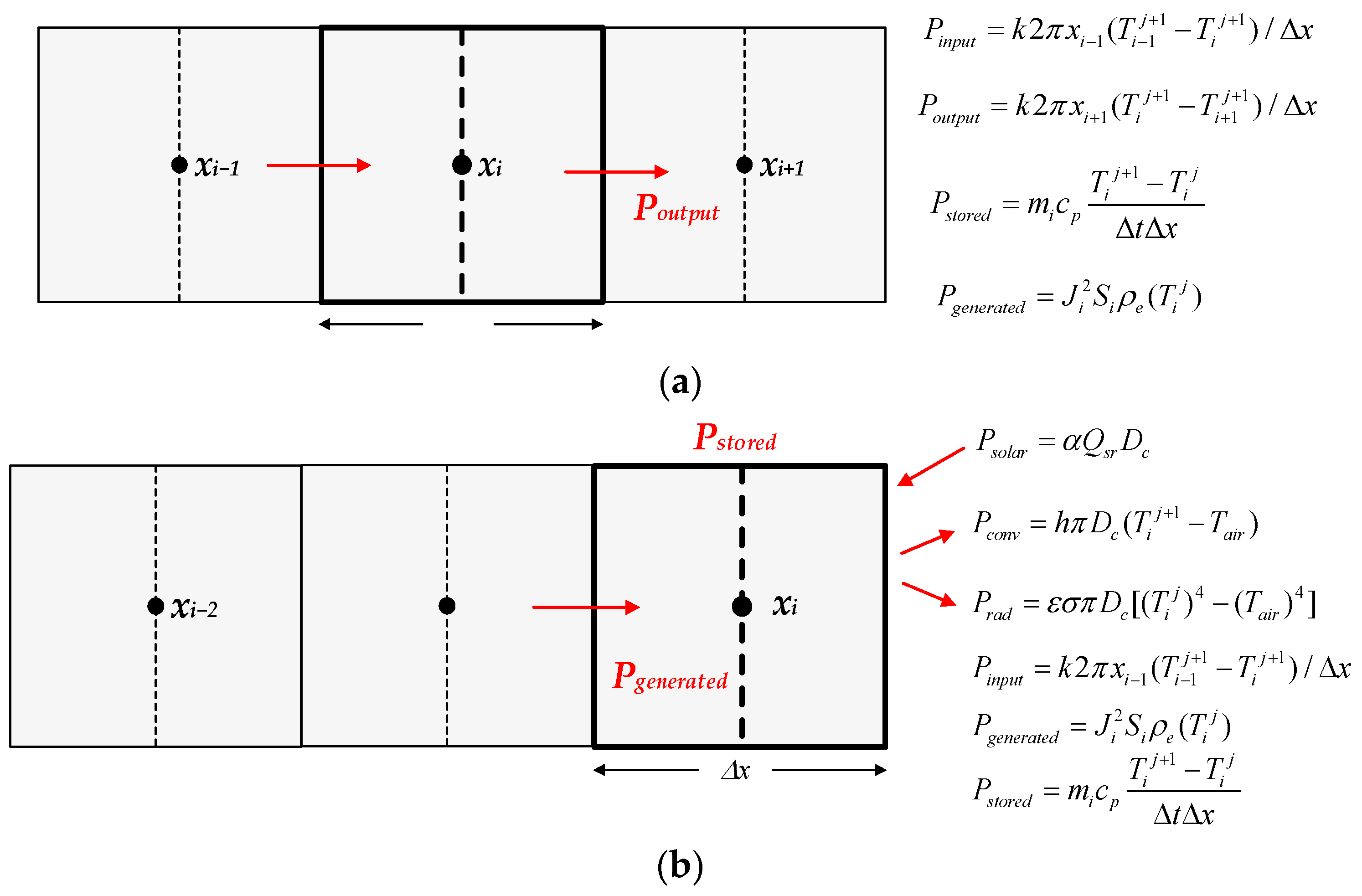
Figure 3 shows the heat balance in a generic inner element and in the outermost element,

3.2. TDMA Formulation

To solve the problem, it is necessary to determine the electrical resistance and the electrical current through each discrete element. Therefore, it is necessary to determine the electrical resistivity ρ_e,i (Ω·m) and the current density J_i = I/S_i (A/m²) in each discrete element, where I (A) and S_i = πx_i² (m²) are the electrical current flowing through the conductor and the cross-sectional area of the discrete element number i, and x_i (m) is the radial position of node i. The resistance per unit length of this discrete element can be calculated as r_i = ρ_e,i/S_i (Ω/m).

The heat transfer equation in a generic element (see Figure 3) can be expressed as,

P_stored = P_generated + P_input − P_output

(15)

Since P_generatred = (J_iS_i)²r_i = J_i²S_iρ_e(T_i^j), the discretized heat transfer equation in a given internal element (there is no solar heating or convective and radiative cooling) can be expressed as,

$$m_i{c}_p\frac{T_i^{j+1}-T_i^j}{\Delta t\Delta x}=J_i^2{S}_i{\rho }_e(T_i^j)+\frac{k2\pi x_{i-1}(T_{i-1}^{j+1}-T_i^{j+1})}{\Delta x}-\frac{k2\pi x_{i+1}(T_i^{j+1}-T_{i+1}^{j+1})}{\Delta x} (\mathrm{W}/\mathrm{m})$$

(16)

where c_p (J/(kgK)) is the specific heat capacity of the material, m_i = ρS_iΔx (kg) is the mass of the i-th discrete element and T_i^j (K) is the absolute temperature of that discrete element at time t = jΔt (s), while ρ (kg/m³) is the volumetric mass density of the material.

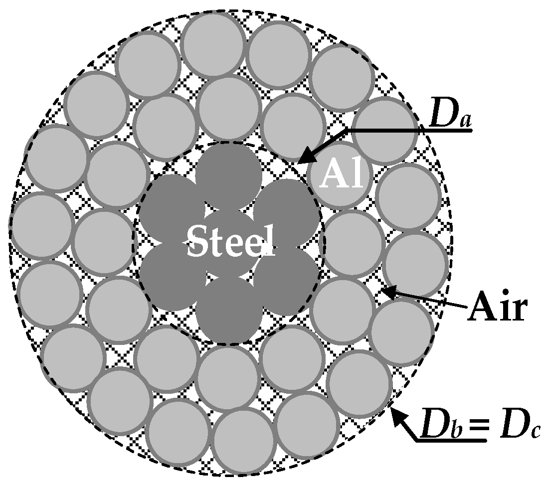
3.3. Particularities of ACSR Conductors

ACSR conductors have a core composed of stainless steel strands and a conductor body composed of aluminum strands, as shown in Figure 4.

Due to the higher electrical conductivity of aluminum, most of the current (approximately 98% [25]) flows through the aluminum strands. The following procedure is used to determine the current densities in the steel core strands and in the aluminum strands. First, the geometric cross-section of the core and the conductor parts can be calculated as S_a = π·D_a²/4 and S_b = π·D_b²/4 − S_a (m²), respectively, where D_a (m) and D_b = D_c (m) are the outer diameters of the core and the aluminum part, respectively. 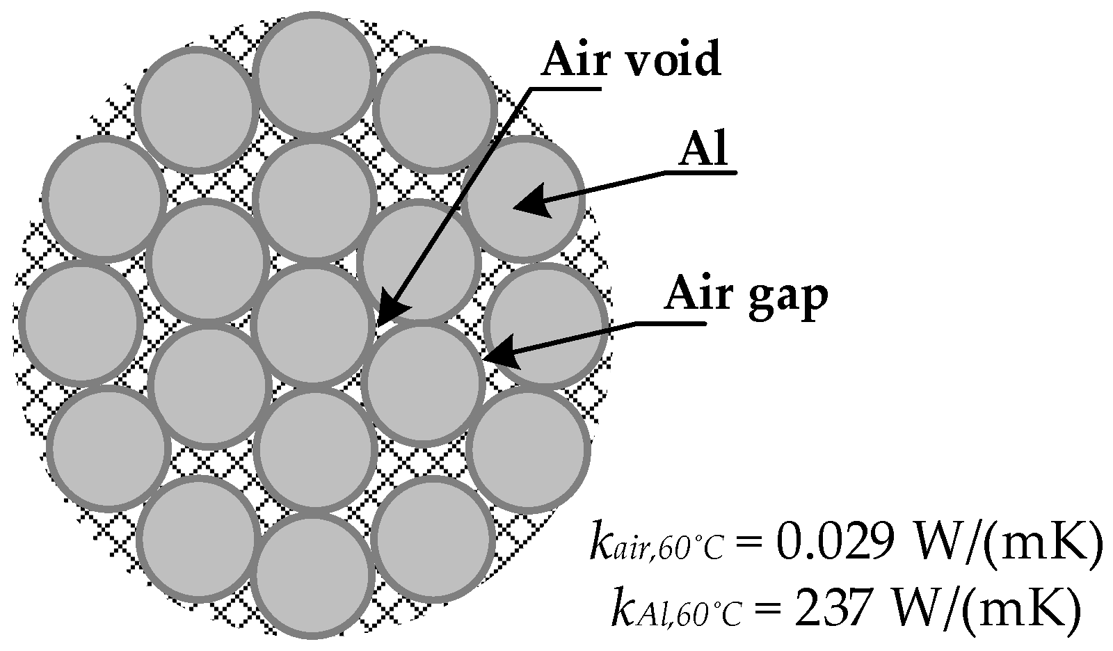It should be noted that the geometric cross-sections S_a and S_b do not coincide with the effective cross-sections of the steel and aluminum parts, S_eff,a and S_eff,b, respectively, due to the air voids and air gaps existing between the strands.

The mass per unit length of the core and the conductor parts, m_a (kg/m) and m_b (kg/m), respectively, are typically specified by the conductor manufacturer. Thus, the mass density of the core and aluminum parts can be determined as ρ_a = m_a/S_a (kg/m³) and ρ_b = m_b/S_b (kg/m³), respectively.

Since the current density through the steel strands is very low, their electrical resistivity can be taken as the tabulated value, ρ_e,a = 6.9 ×·10⁻⁷ Ω·m. However, since the current density through the aluminum strands is high and S_b > S_eff,b, the electrical resistivity of the conductor part used in the calculations can be determined as follows,

$$r_{AC}=\frac{r_a{r}_b}{r_a+r_b}=\frac{\frac{{\rho }_{e,a}}{S_a}·\frac{{\rho }_{e,b}}{S_b}}{\frac{{\rho }_{e,a}}{S_a}+\frac{{\rho }_{e,b}}{S_b}} [\Omega /\mathrm{m}] \to {\rho }_{e,b}=r_{AC}\frac{{\rho }_{e,a}{S}_b}{{\rho }_{e,a}-r_{AC}{S}_a}$$

(17)

where r_AC (Ω/m) is the AC resistance per unit length of the conductor, which includes the effects of eddy currents and core losses. Note that (17) is derived from the parallel between the electrical resistances per unit length of the core r_a and the conductive part r_b. Once the resistivity ρ_e,a and ρ_e,b of both parts are known, the currents i_a and i_b in each part of the conductor can be calculated as,

r_a(t) = ρ_e,a,To · [1 + α_a,AC(T(t) − T₀)]/S_a, r_b(t) = ρ_e,b,To · [1 + α_b,AC(T(t) − T₀)]/S_b (Ω/m)

(18)

i_a(t) = i(t)·r_b(t)/[r_a(t) + r_b(t)], i_b(t) = i(t)·r_a(t)/[r_a(t) + r_b(t)] (A)

(19)

J_a(t) = i_a(t)/S_a, J_b(t) = i_b(i)/S_b (A/m²)

(20)

4. Effective Radial Thermal Conductivity k_r,eff, Its Determination and Published Values

4.1. Effective Radial Thermal Conductivity k_r,eff

The heat generated in the inner layers of the conductor due to i²r_AC is conducted radially along the contact surface from one strand to the next until it reaches the outer surface [22,34], so a radial thermal gradient is expected. When it reaches the conductor surface, this heat is dissipated to the surrounding atmospheric air primarily by convection and, to a lesser extent, by radiation. Under transient conditions, some of the heat may be stored in the conductor. The radial temperature difference between the center and the surface of the conductor depends on the conductor geometry (stranding and number of layers), the current level, the electrical resistance and the effective radial thermal conductivity [19].

As shown in Figure 5, transmission line conductors are not solid, but stranded, which makes the physics of the problem more complex.

According to [20,22], in multilayer stranded conductors, most of the i²r_AC heat flow is conducted radially through the air voids that exist between strands in adjacent layers and through the air gaps that exist at the contact area between strands in adjacent layers, as shown in Figure 5. Internal convective and radiative effects are negligible, and the contact area between adjacent wires increases with the tension in the conductor [20]. The contact area depends on corrosion effects and accumulated grease. Therefore, the effective radial thermal conductivity k_r,eff (W/(mK)) of the conductor is greatly reduced and is much lower than the thermal conductivity of the aluminum material [35]. This is because the thermal conductivity of air is several orders of magnitude lower than that of the aluminum strands (see Figure 5), resulting in k_r,eff ~ k_Al/100 due to the resistance to radial heat flow of the air voids and the interstrand contact [17]. It is also known that for constant current operation, k_r,eff increases (i.e., the radial temperature difference decreases) with increasing values of the mechanical axial tension, interlayer contact pressure and air pressure [22] and with a decreasing degree of corrosion [19]. Conductors with fewer layers and higher wind speeds also tend to increase k_r,eff [36].

Thermal conductivity measurements of stranded conductors in indoor and outdoor environments are extremely difficult due to the measurement variability associated with the measurement technique [36]. In real applications, the situation is even worse because there are many factors that affect k_r,eff. In addition, it is impractical to measure the radial temperature distribution inside the conductor in real applications, so it is important to generate accurate conductor models that take into account the temperature distribution inside the conductor.

4.2. Determination of the Radial Thermal Conductivity k_r,eff

According to several references [11,12,19], in the steady state, the radial temperature difference ΔT(r) is directly proportional to P_internal = i²r_AC and inversely proportional to the effective radial thermal conductivity k_r,eff as,

$$\Delta T(r)=T(r)-T_s=\frac{i^2{r}_{AC}(T_{average})}{2\pi k_{r,eff}}\left[\frac{r_s^2-r^2}{2(r_s^2-r_c^2)}+\frac{r_c^2}{r_s^2-r_c^2}\ln (r/r_s)\right]$$

(21)

From (21), the effective thermal conductivity k_eff of the conductor can be determined as [19],

$$k_{r,eff}=\frac{i^2{r}_{AC}(T_{average})}{2\pi [T(r)-T_s]}\left[\frac{r_s^2-r^2}{2(r_s^2-r_c^2)}+\frac{r_c^2}{r_s^2-r_c^2}\ln (r/r_s)\right]$$

(22)

In the case of all aluminum conductors, since r_c = 0, the above equations are simpler [17],

$$\Delta T(r=0)=T(r=0)-T_s=\frac{i^2{r}_{AC}(T_{average})}{4\pi k_{r,eff}}$$

(23)

$$k_{r,eff}=\frac{i^2{r}_{AC}(T_{average})}{4\pi [T(r=0)-T_s]}$$

(24)

From (24), k_r,eff can be determined if i²r_AC and the total radial temperature gradient are known [20].

In [17], the following expression for the radial temperature gradient was obtained by solving the heat equation of a homogeneous and symmetric cylindrical conductor,

$$\Delta T(r)=T(r)-T_s=\frac{i^2{r}_{AC}(T_{average})}{4\pi k_{r,eff}}\left[1-{\left(\frac{r}{r_s}\right)}^2\right]$$

(25)

which also leads to (23) when r = 0. Note that (23)–(25) assume that the electrical resistance of the conductor is constant throughout its cross-section despite the small radial thermal gradients.

4.3. Published Values of the Radial Thermal Conductivity k_r,eff

As explained above, published works suggest that reasonable values of k_r,eff are in the range of 0.5–4.0 W/(mK), and in the case of ACSR conductors at moderate current densities, Refs. [11,12,35] suggest k_r,eff ≈ 2 W/(mK) for aluminum strands, while in the case of ACSR conductors under little or no applied tension, k_r,eff ≈ 1 W/(mK). Ref. [35] suggests that k_r,eff ≈ 1.5 W/(mK) for steel strands. A bibliographic review presented in [19] analyzing various conductors suggests values of k_r,eff in the range of 1.2–10.0 W/(mK). Analyzing an all-aluminum conductor (AAC) with an outer diameter of 44.45 mm and 91 aluminum strands of 4.04 mm each, Morgan [22] suggested that k_r,eff ≈ 0.7–1.1 W/(mK) under axial tensions of 4.45–22.2 kN. In [37], values of k_r,eff = 0.98 W/(mK) are reported for a Cardinal ACSR conductor and k_r,eff = 4 W/(mK) for a Marigold AAC conductor. In [19], values of k_r,eff ≈ 1.34–1.90 W/(mK) are reported for different types of copper conductors, k_r,eff ≈ 2.10–2.86 W/(mK) for different AAC conductors, k_r,eff ≈ 1.86–4.47 W/(mK) for different AAAC conductors, and k_r,eff ≈ 2.46–4.70 W/(mK) for different ACSR conductors.

The value of k_r,eff is strongly influenced by the factors that determine the amount of air trapped between the strands, such as conductor topology, number of layers, strand geometry (round versus trapezoidal) or conductor temperature, since an excessive temperature will cause separation between adjacent strands, known as birdcaging [35]. For a specific application, its value can be approximated from the tabulated values or by fitting experimental test data to simulation results obtained with the radial model proposed in this paper.

For stranded conductors operating below the SLR limit, the temperature gradient between the surface and the center of the conductor is much smaller than the conductor temperature increase over the ambient temperature. However, below the DLR limit, and for new applications such as HTLS conductors, the radial temperature gradients may not be negligible [17].

5. Radial Problem Formulation

This section develops the equations to solve the problem using a one-dimensional radial formulation.

5.1. Analysis of Node i = 1 Belonging to the Core (Material a)

If the core is conductive, node i = 1 generates heat due to the internal losses, which is conducted outward to node i = 2. The discrete form of the transient heat transfer Equation (16) applied to node i = 1 is as follows,

$${\rho }_a\pi {(x_1+0.5\Delta x_a)}^2{c}_{p,a}\Delta x_a\frac{T_1^{j+1}-T_1^j}{\Delta t\Delta x_a}=J_{i,a}^2{S}_{i,a}{\rho }_{e,a}(T_i^j)-\frac{k_{a}2\pi (x_1+0.5\Delta x_a)(T_1^{j+1}-T_2^{j+1})}{\Delta x_a}$$

(26)

The terms in (26) can be rearranged as needed in the TDMA formulation (11), so that for the first node becomes

$$a_1=0, b_1=\frac{{\rho }_a\pi {(x_1+0.5\Delta x_a)}^2{c}_{p,a}}{\Delta t}+\frac{k_{a}2\pi (x_1+0.5\Delta x_a)}{\Delta x_a}, c_1=-\frac{k_{a}2\pi (x_1+0.5\Delta x_a)}{\Delta x_a}, d_1=\frac{{\rho }_a\pi {(x_1+0.5\Delta x_a)}^2{c}_{p,a}{T}_1^j}{\Delta t}+J_{i,a}^2{S}_{i,a}{\rho }_{e,a}(T_i^j)$$

(27)

For conductors with a non-conducting core, such as aluminum conductor composite core (ACCC) conductors, J_i,a = 0 must be used in (26) and (27).

5.2. Analysis of a Generic Node 2 ≤ i ≤ N_a Belonging to the Core (Material a)

This generic node has an area S_i,a = π(x_i + 0.5Δx_a)² − π(x_i − 0.5Δx_a)² = 2πx_iΔx_a. When evaluating the heat transfer in this generic node i, we must take into account the heat generation term, the heat input heat conducted from the left or inner element and the output heat conducted to the right or outer element, resulting in,

$${\rho }_{a}2\pi x_i\Delta x_a{c}_{p,a}\Delta x_a\frac{T_i^{j+1}-T_i^j}{\Delta t\Delta x_a}=J_{i,a}^2{S}_{i,a}{\rho }_{e,a}(T_i^j)+\frac{k_{a}2\pi (x_i-0.5\Delta x_a)(T_{i-1}^{j+1}-T_i^{j+1})}{\Delta x_a}-\frac{k_{a}2\pi (x_i+0.5\Delta x_a)(T_i^{j+1}-T_{i+1}^{j+1})}{\Delta x_a}$$

(28)

The TDMA coefficients are obtained from (28) as,

$$a_i=-\frac{k_{a}2\pi (x_i-0.5\Delta x_a)}{\Delta x_a}, b_i=\frac{{\rho }_{a}2\pi x_i\Delta x_a{c}_{p,a}}{\Delta t}+\frac{k_{a}4\pi x_i}{\Delta x_a}, c_i=-\frac{k_{a}2\pi (x_i+0.5\Delta x_a)}{\Delta x_a}, d_i=\frac{{\rho }_{a}2\pi x_i\Delta x_a{c}_{p,a}{T}_i^j}{\Delta t}+J_{i,a}^2{S}_{i,a}{\rho }_{e,a}(T_i^j)$$

(29)

5.3. Analysis of the Boundary Node between the Core and the Conductor (i = N_a)

The formulation of this node is similar to that in (28), taking into account the different thermal conductivities (k_a and k_b) and electrical resistivities (ρ_e,a and ρ_e,b) on either side of the boundary,

$${\rho }_a{S}_{i,a}{c}_{p,a}\frac{T_i^{j+1}-T_i^j}{\Delta t}+{\rho }_b{S}_{i,b}{c}_{p,b}\frac{T_i^{j+1}-T_i^j}{\Delta t}=J_{i,a}^2{S}_{i,a}{\rho }_{e,a}(T_i^j)+J_{i,b}^2{S}_{i,b}{\rho }_{e,b}(T_i^j)+\frac{k_{a}2\pi (x_i-0.5\Delta x_a)(T_{i-1}^{j+1}-T_i^{j+1})}{\Delta x_a}-\frac{k_{b}2\pi (x_i+0.5\Delta x_b)(T_i^{j+1}-T_{i+1}^{j+1})}{\Delta x_b}$$

(30)

where S_i,a = π(x_i)² − π(x_i − 0.5Δx_a)² and S_i,b = π(x_i + 0.5Δx_b)² − π(x_i)². The TDMA coefficients in this boundary are as follows,

$$\begin{array}{l}{a}_i=-\frac{k_{a}2\pi (x_i-0.5\Delta x_a)}{\Delta x_a}, b_i=\frac{{\rho }_a{S}_{i,a}{c}_{p,a}}{\Delta t}+\frac{{\rho }_b{S}_{i,b}{c}_{p,b}}{\Delta t}+\frac{k_{a}2\pi (x_i-0.5\Delta x_a)}{\Delta x_a}+\frac{k_{b}2\pi (x_i+0.5\Delta x_b)}{\Delta x_b},\\ c_i=-\frac{k_{b}2\pi (x_i+0.5\Delta x_b)}{\Delta x_b}, d_i=\frac{{\rho }_a{S}_{i,a}{c}_{p,a}{T}_i^j}{\Delta t}+\frac{{\rho }_b{S}_{i,b}{c}_{p,b}{T}_i^j}{\Delta t}+J_{i,a}^2{S}_{i,a}{\rho }_{e,a}(T_i^j)+J_{i,b}^2{S}_{i,b}{\rho }_{e,b}(T_i^j)\end{array}$$

(31)

In the case of single-material conductors, such as all-aluminum alloy conductors (AAAC), k_a = k_b, c_p,a = c_p,b and ρ_e,a = ρ_e,b.

5.4. Analysis of a Generic Node N_a + 1 ≤ i ≤ N_a + N_b Belonging to the Conductor (Material b)

This formulation is similar to that in the generic node belonging to the core (2 ≤ i ≤ N_a), but the subscripts a are replaced by subscripts b,

$${\rho }_{b}2\pi x_i\Delta x_b{c}_{p,b}\Delta x_b\frac{T_i^{j+1}-T_i^j}{\Delta t\Delta x_b}=J_{i,b}^2{S}_{i,b}{\rho }_{e,b}(T_i^j)+\frac{k_{b}2\pi (x_i-0.5\Delta x_b)(T_{i-1}^{j+1}-T_i^{j+1})}{\Delta x_b}-\frac{k_{b}2\pi (x_i+0.5\Delta x_b)(T_i^{j+1}-T_{i+1}^{j+1})}{\Delta x_b}$$

(32)

The TDMA coefficients are obtained from (32) as,

$$a_i=-\frac{k_{b}2\pi (x_i-0.5\Delta x_b)}{\Delta x_b}, b_i=\frac{{\rho }_{b}2\pi x_i\Delta x_b{c}_{p,b}}{\Delta t}+\frac{k_{b}4\pi x_i}{\Delta x_b}, c_i=-\frac{k_{b}2\pi (x_i+0.5\Delta x_b)}{\Delta x_b}, d_i=\frac{{\rho }_{b}2\pi x_i\Delta x_b{c}_{p,b}{T}_i^j}{\Delta t}+J_{i,b}^2{S}_{i,b}{\rho }_{e,b}(T_i^j)$$

(33)

5.5. Analysis of the Boundary Node between the Conductor and the Air (i = N_a + N_b + 1)

Assuming Δx_air = Δx_b, this boundary node has an area S_i,a = π(x_i)² − π(x_i − 0.5Δx_b)² = πΔx_air(x_i − 0.25Δx_b), as shown in Figure 3. This is the outermost node, which is placed in the boundary between the conductor and the air, so in the absence of wind (worst case), heating by solar radiation and radiative and convective cooling effects must be considered, resulting in,

$$\begin{array}{c}{\rho }_b\pi \Delta x_b(x_i-0.25\Delta x_b)c_{p,b}\Delta x_b\frac{T_i^{j+1}-T_i^j}{\Delta t\Delta x_b}=\\ =\frac{k_{b}2\pi (x_i-0.5\Delta x_b)(T_{i-1}^{j+1}-T_i^{j+1})}{\Delta x_b}+J_{i,b}^2{S}_{i,b}{\rho }_{e,b}(T_i^j)+\alpha Q_{sr}{D}_c-h\pi D_c(T_i^{j+1}-T_{air})-\epsilon \sigma \pi D_c[{(T_i^j)}^4-{(T_{air})}^4]\end{array}$$

(34)

Finally, the TDMA coefficients of the outermost boundary node are as follows,

$$\begin{array}{c}{a}_i=-\frac{k_{b}2\pi (x_i-0.5\Delta x_b)}{\Delta x_b}, b_i=\frac{{\rho }_b\pi \Delta x_b(x_i-0.25\Delta x_b)c_{p,b}}{\Delta t}+\frac{k_{b}2\pi (x_i-0.5\Delta x_b)}{\Delta x_b}+h\pi D_c\\ c_i=0, d_i=\frac{{\rho }_b\pi \Delta x_b(x_i-0.25\Delta x_b)c_{p,b}{T}_i^j}{\Delta t}+J_{i,b}^2{S}_{i,b}{\rho }_{e,b}(T_i^j)+\alpha Q_{sr}{D}_c+h\pi D_c{T}_{air}-\epsilon \sigma \pi D_c[{(T_i^j)}^4-{(T_{air})}^4]\end{array}$$

(35)

This code was programmed by the authors of this paper using Matlab^® R2022b.

6. Conductors Analyzed and Experimental Setup

To validate and evaluate the accuracy of the proposed radial model, this paper analyzes three different conductors, an all-aluminum alloy conductor (AAAC), an ACSR conductor and a high-temperature low-sag (HTLS) conductor, which are described in the following sections.

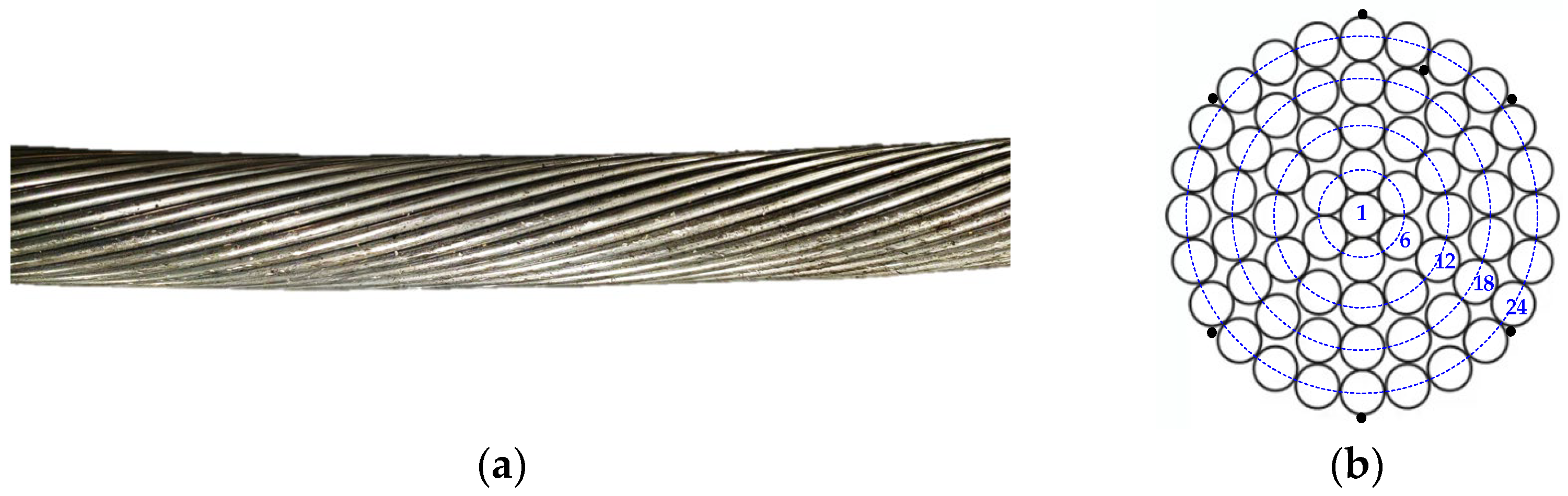
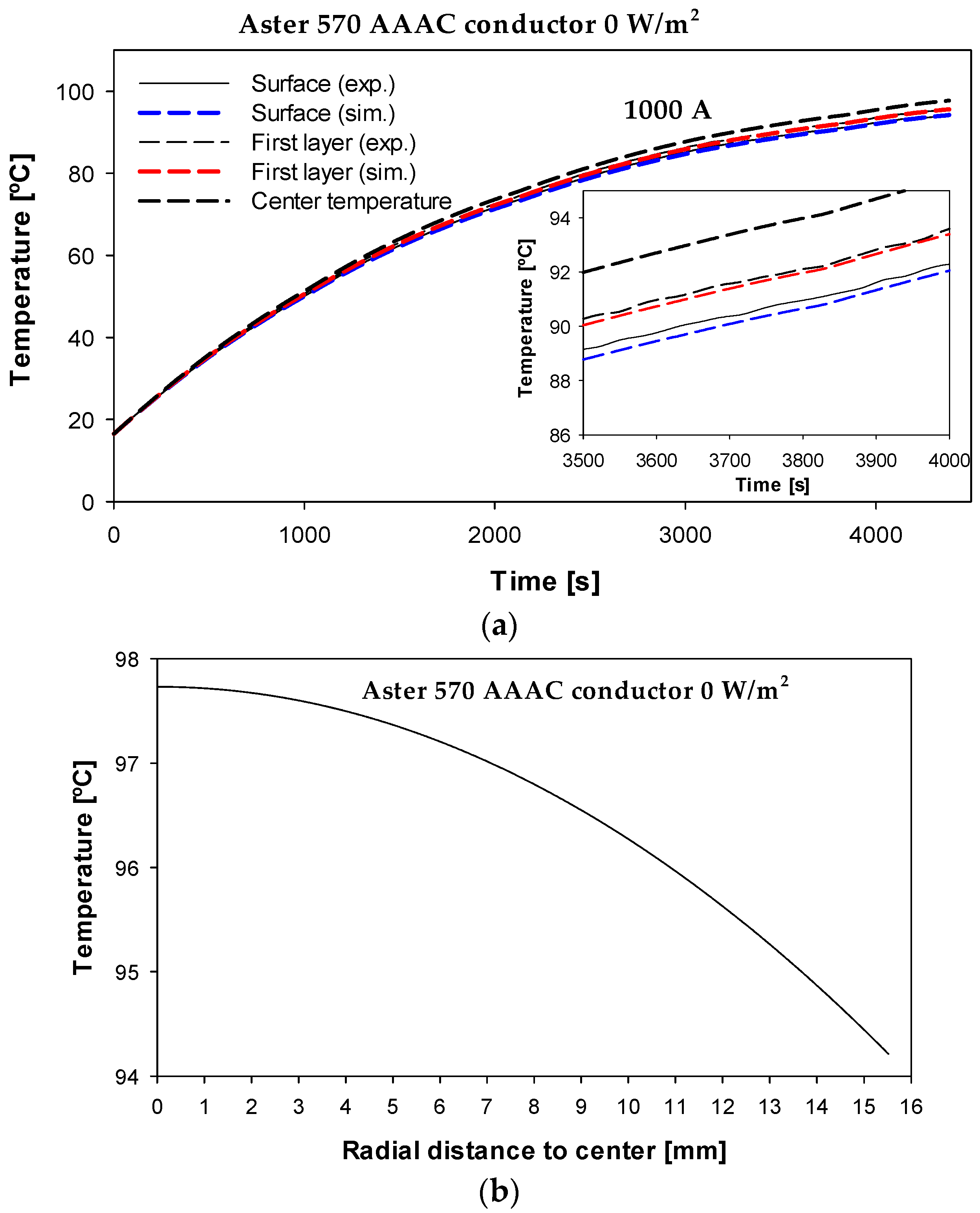
6.1. AAAC Conductors

AAAC conductors use a high-strength aluminum alloy to achieve good sag characteristics and a high strength-to-weight ratio. All strands are made of high-strength aluminum alloy, so there is no steel core. AAAC conductors offer higher corrosion resistance compared to ACSR conductors.

This paper analyzes the thermal behavior of the Aster 570 AAAC conductor, which has 61 aluminum strands and a 1/6/12/18/24 distribution, as shown in Figure 6.

Table 1. Main parameters of the Aster 570 AAAC conductor.

Input Parameters	Units	Aster 570 AAAC Conductor
Number of strands	(-)	61
Strand diameter	(mm)	3.45
Outer diameter	(mm)	31.05
Effective conductor cross-section	(mm2)	570.22
Conductor emissivity	(-)	0.25
Effective radial thermal conductivity	(W/(mK))	2.0
AC resistance per unit length at 20 °C	(Ω/km)	0.06763
Temperature coefficient of resistance	(K−1)	0.0036
Density of conductor material	(kg/m3)	2700 (Al)
Mass per unit length	(kg/m)	1.576
Emissivity	(-)	0.25

shows the main parameters of the Aster 570 AAAC conductor.

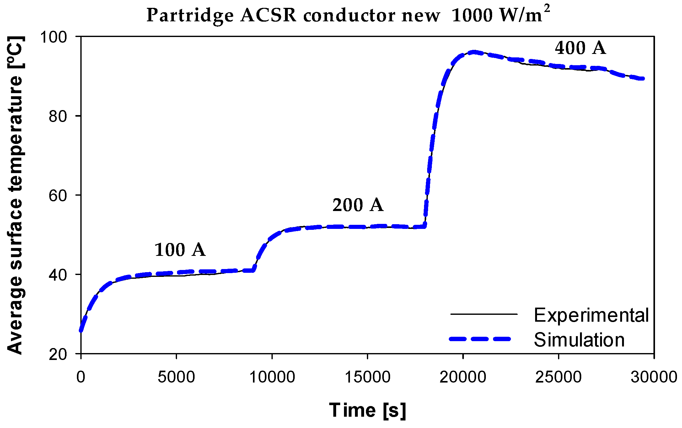
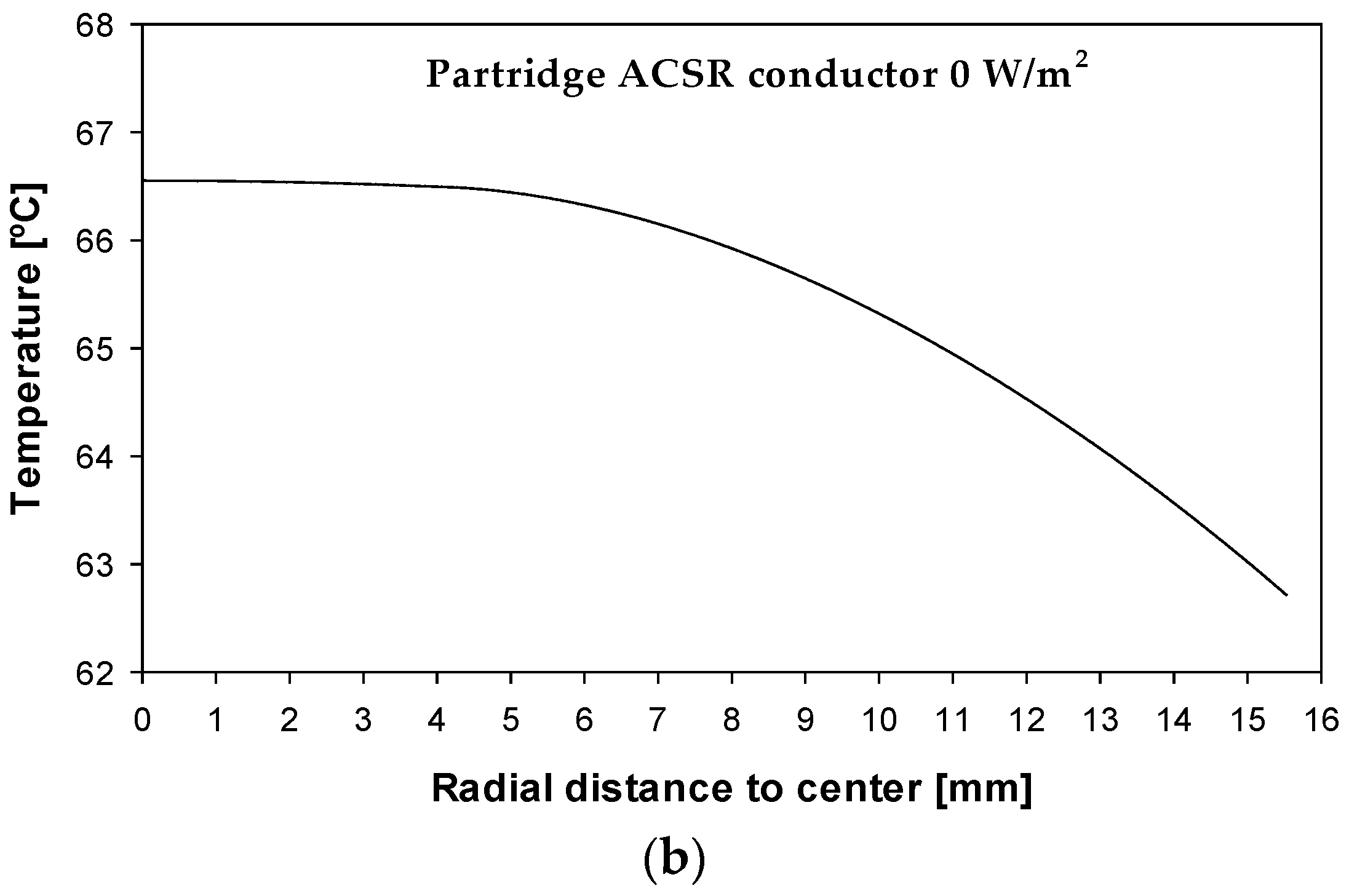
6.2. ACSR Conductors

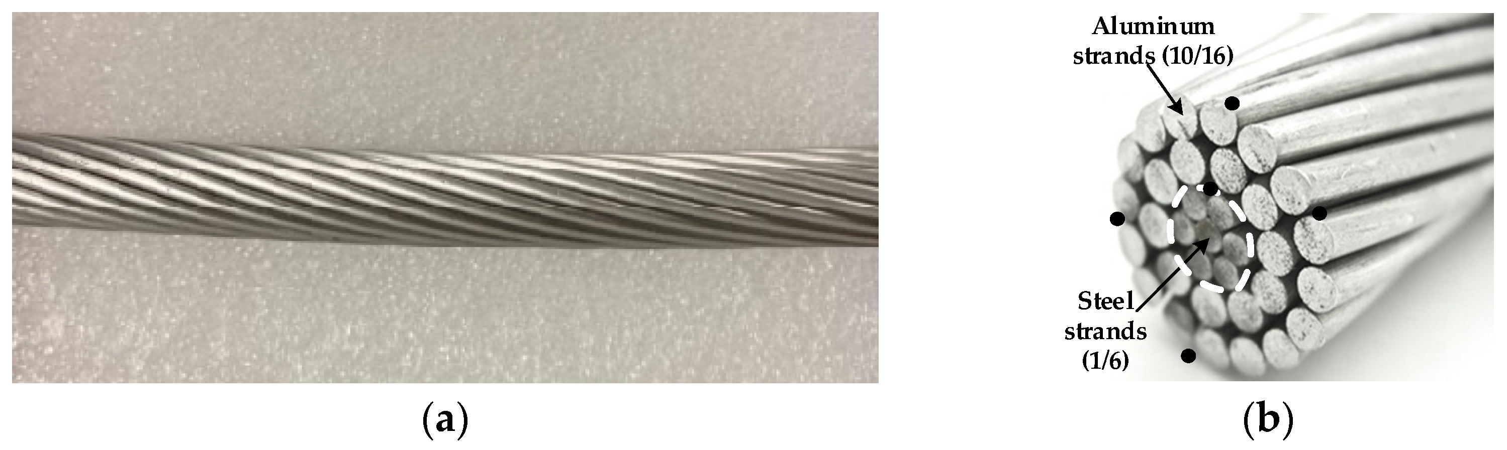
As explained above, ACSR conductors consist of multiple layers of aluminum strands wound helically around an inner core made of galvanized steel strands. While the aluminum strands carry most of the electrical current, the steel strands provide the mechanical strength. This paper also analyzes the thermal behavior of a two-layer ACSR conductor (Partridge 135-AL1/22-ST1A, EMTA Kablo, Istanbul, Turkey). This conductor has a steel core with seven steel strands (1/6 steel configuration) and two conductive aluminum layers with 10 and 16 aluminum strands (10/16 aluminum configuration).

Figure 7 shows the Partridge 135-AL1/22-ST1A ACSR conductor.

Table 2. Main parameters of the new two-layer Partridge 135-AL1/22-ST1A ACSR conductor.

Description	Unit	Value
AC resistance per unit length at 20 °C	(Ω/km)	0.2038
Temperature coefficient of resistance	(K−1)	0.0035
Current carrying capacity	(A)	430
Number of aluminum strands	(-)	26 (10/16)
Number of steel strands	(-)	7 (1/6)
Aluminum strand diameter	(mm)	2.57
Steel wire diameter	(mm)	2.0
Outer diameter	(mm)	16.3
Aluminum area	(mm2)	134.9
Steel area	(mm2)	22.0
Mass per unit length	(kg/m)	0.5445
Core mass per unit length	(kg/m)	0.1728
Aluminum mass per unit length	(kg/m)	0.3717
Effective radial thermal conductivity of Al part	(W/(mK))	2.0
Effective radial thermal conductivity of steel part	(W/(mK))	1.5
Emissivity	(-)	0.26

shows the main parameters of the Partridge 135-AL1/22-ST1A ACSR conductor, which consists of 7 steel strands with a 1/6 distribution and 26 aluminum strands with a 10/16 distribution.

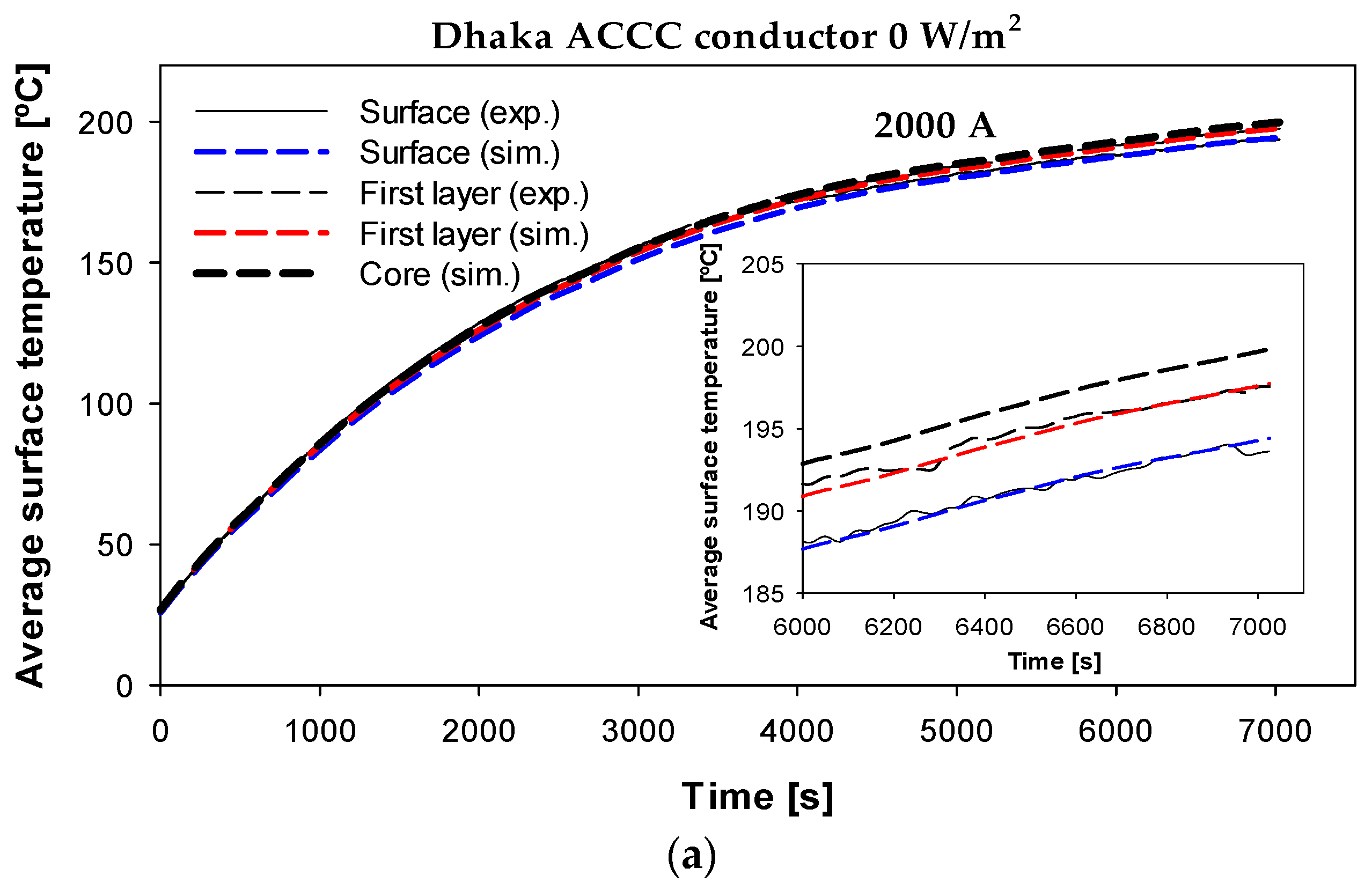
6.3. HTLS Conductors

An HTLS conductor-type aluminum conductor composite core (ACCC) with trapezoidal wire (TW), also known as ACCC/TW, was analyzed. To limit sag at high temperatures, this HTLS conductor has a non-conductive, lightweight and high-strength hybrid core of carbon and glass fibers embedded in a resin matrix [38]. Fully annealed and helically wound trapezoidal aluminum strands surround the hybrid core. These fully annealed aluminum strands are purer and more conductive than the strands used in conventional ACSR conductors. The continuous operating temperature of these conductors is approximately 180 °C [39]. Figure 8 shows the cross-section of the ACCC/TW used in this work and the location of the thermocouples (black dots).

Table 3. Main parameters of the three-layer Dhaka ACCC/TW conductor.

Description	Unit	Two-Layer
AC resistance per unit length at 20 °C	(Ω/km)	0.03984
Temperature coefficient of resistance	(K−1)	0.0040
Current carrying capacity	(A)	2000
Number of aluminum strands	(-)	36 (8/12/16)
Outer diameter	(mm)	34.45
Core diameter	(mm)	9.53
Aluminum area	(mm2)	723.9
Mass per unit length	(kg/m)	2.137
Core mass per unit length	(kg/m)	0.132
Aluminum mass per unit length	(kg/m)	2.005
Effective radial thermal conductivity	(W/(mK))	4.0
Emissivity	(-)	0.4

shows the main parameters of the three-layer Dhaka ACCC/TW conductor.

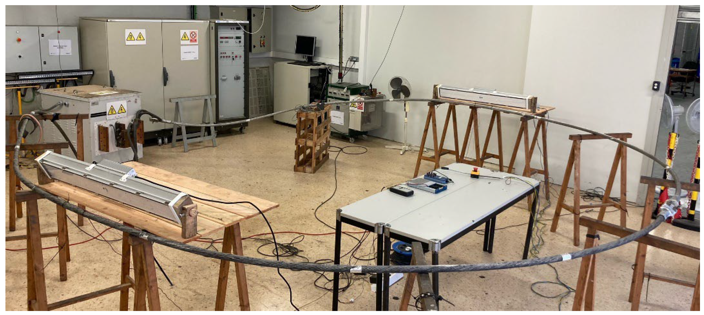
6.4. Experimental Setup

The tests were performed in an indoor high-current laboratory. All tested conductors were connected to the output of the high-current transformer (0–10 V output voltage, 0–10 kA output current), forming a low-impedance loop.

Since the experiments were conducted indoors, LED projectors (Series AGRO-K, average photosynthetic photon flux density 430 μMol/m²/s, Venalsol, Valencia, Spain) were used to simulate the solar irradiance. The global solar irradiance was measured with a global radiation meter (PCE-SPM 1, silicon sensor, 400–1100 nm, 0–2000 W/m², 0.1 W/m², accuracy ± 10 W/m², PCE Instruments, Southampton, UK).

The AC resistance per unit length r_AC of the conductors was determined experimentally from (5) by measuring the voltage drop across a 1 m length of conductor and the phase shift between the voltage drop and the current.

The current flowing through the loop was measured with a Rogowski coil (CWT500LFxB, 0.06 mV/A sensitivity, ±1% current accuracy, PEM, Nottingham, UK). The data provided by the Rogowski coil and the voltage drop in the conductors were acquired using an NI USB-6343 data acquisition card (National Instruments, Dallas, TX, USA), from which the phase shift between the voltage drop and the current can be determined, and thus the AC resistance per unit length r_AC.

Low inertia T-type thermocouples were used to measure the surface temperature of the conductors. The data provided by the thermocouples was acquired using a thermocouple input module (TC08, ±1 °C, Omega, Northbank, Manchester, UK).

A Python code was used to synchronize the measurements taken with the TC08 thermocouple input module and the NI USB-6343 data acquisition card.

The experimental setup is shown in Figure 9.

To avoid heat sink effects from the edges, the conductors were long enough (about 8–10 m each) and measurements were made in the center of the conductor [17].

Different thermocouples were placed on the outer surface of each conductor to determine the average surface temperature. To measure the internal temperature, thermocouples were also implanted directly into different layers of the conductor, forcing adjacent strands to open and taking care not to deform the geometry of the conductor once in place. Thermal paste was used to improve the thermal contact between the thermocouples and the aluminum strands. The test setup was located indoors, which allowed measurements to be made at zero wind speed.

7. Radial Temperature Profile and Model Validation from Experimental Results

This section presents experimental results, which are used to validate the simulation model presented in Section 5.

7.1. ASTER 570 AAAC Conductor

This section validates the simulation model with experimental results using the ASTER 570 AAAC conductor. Simulation models are attractive because they can provide results very close to experimental results in a faster, less expensive and more environmentally friendly manner. Figure 10 compares the experimental and simulation results obtained with the Aster 570 conductor using different currents (220–520–1000 A) and a solar irradiance of 0 W/m² and 1000 W/m².

The results presented in Figure 10 show a great similarity between the experimental and simulation results. Although two solar irradiance conditions were tested and simulated, i.e., 0 W/m² and 1000 W/m², in both cases, the simulation results were very close to the experimental ones, which allows us to validate the simulation model presented in Section 5. It should be noted that Figure 10 shows the average readings of the different thermocouples placed on the surface of the conductor. It should be noted that the proposed radial model assumes a uniform surface temperature distribution, although the laboratory results indicate that the higher temperature corresponds to the lowest point, while the lower temperature of the surface corresponds to the highest point.

To further validate the simulation model, the surface temperature and the temperature at the interface between the outer layer and the second layer were measured when a step current of 1000 A was applied without solar radiation. The experimental and simulated results are shown in Figure 11. Note that the experimental value of the surface temperature is the average of the readings from the different thermocouples placed on the outer surface.

The results shown in Figure 11a again show a strong similarity between experimental and simulation results. The results shown in Figure 11b predict a temperature gradient of about 3.5 °C between the center and the surface of the conductor under the operating conditions shown in Figure 11, while the calculated temperature difference from (25) was 3.4 °C. The average temperature difference between the experimental results and the simulation results was 0.32% and 0.38% for the surface and first layer temperatures, respectively.

7.2. Partridge 135-AL1/22-ST1A ACSR Conductor

Further validation of the simulation model was performed on the 135-AL1/22-ST1A ACSR conductor. Figure 12 compares the experimental and simulation results obtained with the Aster 570 conductor at different currents (100–200–400 A) and 1000 W/m² of solar irradiance.

The results shown in Figure 12 also show a great similarity between the experimental and simulation results. These results are particularly relevant due to the inherent complexity of ACSR conductors composed of two materials, i.e., the magnetic core of galvanized steel strands and the aluminum strands. These results further validate the accuracy of the proposed radial model.

Next, the surface temperature and the temperature at the interface between the second layer and the core were measured when a step current of 285 A was applied in the absence of solar radiation. The experimental and simulated results are shown in Figure 13, which again shows a great similarity between the experimental and simulated results.

The results shown in Figure 13b predict a temperature gradient of about 3.8 °C between the core and the surface of the conductor under the operating conditions shown in Figure 13, while the calculated temperature difference from (21) was 3.6 °C. The average temperature difference between the experimental and simulation results was 0.61% and 0.54% for the surface and core temperatures, respectively.

7.3. Dhaka HTLS Conductor

Finally, to further validate the simulation model for high-temperature operations, the Dhaka HTLS conductor was tested under a step current of 2000 A. The surface temperature and the temperature at the interface between the first and second outermost layers were measured. The experimental and simulated results are presented in Figure 14, which again shows a great similarity between the experimental and simulated results, even at high-temperature operation.

The results shown in Figure 14b predict a temperature gradient of about 4.4 °C between the core and the surface of the conductor under the operating conditions shown in Figure 14, almost the same temperature difference calculated from (21). The average temperature difference between experimental and simulation results was 1.13% and 1.00% for the surface and first layer temperatures, respectively. It should be noted that ACCC conductors are challenging because they operate at very high temperatures and have a non-conductive hybrid composite core. Nevertheless, the proposed radial model reproduces the experimental laboratory results with high accuracy.

7.4. Comparative Results of the Proposed Radial Model versus the Classical Model

This section analyzes the accuracy of the proposed radial method in comparison with the classical model that assumes a homogeneous temperature inside the conductor, which is equivalent to assuming infinite thermal conductivity of the conductor material. The results obtained are summarized in

Table 4. Average difference between the laboratory experimental results and simulation results obtained with the proposed radial model and the classical homogeneous model.

Conductor	Data Origin	Average Difference
		Radial Model	Classical Model
Aster A570 AAAC	Figure 11	0.32%	0.40%
Partridge ACSR	Figure 13	0.61%	0.97%
Dhaka ACCC/TW	Figure 14	1.13%	1.20%

.

The results presented in Table 4 show that although both models are accurate, the radial model gives results more similar to the experimental ones for the three conductors analyzed in this work operating under different conditions.

Finally, it should be emphasized that in order to show the accuracy of the proposed model, three types of conductors with very different characteristics have been analyzed, namely an all-aluminum alloy conductor (AAAC), an ACSR conductor and an ACCC (HTLS) conductor. The AAAC conductor is composed of aluminum strands only, while the two other two conductors are composed of two materials. While ACSR conductors have a magnetic core made of galvanized steel strands, ACCC conductors have a non-conductive hybrid composite core. Despite the different types of conductors, the different solar radiation conditions, the different current densities studied and the different temperature ranges achieved, the simulation results obtained with the proposed radial model are very close to the experimental laboratory results. Therefore, it can be concluded that this radial model can be effectively used for the purposes of DLR.

8. Conclusions

Stranded conductors are critical elements of overhead power lines. A radial thermal gradient is created as the internal heat generated is conducted to the outer surface. In order to fully utilize the current-carrying capacity of the conductor and to ensure safe operation, e.g., when developing accurate conductor line models to apply dynamic line rating (DLR) strategies, this effect must be taken into account because two important terms of the heat transfer equation—i.e., the internal heating, which is the main source of heating, and the stored heat, which strongly affects the dynamics of the heat transfer—depend on the internal temperature distribution. In addition, annealing, creep and sag effects are strongly influenced by the radial temperature distribution within the conductor. Therefore, accurate thermoelectric conductor models must take into account the temperature distribution within the conductor.

This paper has presented a radial one-dimensional thermoelectric model for bare-stranded conductors. The accuracy of the proposed model has been evaluated through experimental tests performed on three types of conductors, namely AAAC, ACSR and ACCC-HTLS conductors. The experimental results presented in this paper show that the thermal gradient between the center and the outer surface of the conductor can be predicted with accuracy using the proposed radial one-dimensional model, which improves the capabilities of the models proposed in the IEC, Cigré and IEEE standards, especially when designing DLR approaches. In particular, the results presented under different conditions (varying current density, solar irradiance and temperature range) show that the average differences between the laboratory results and the results of the radial model are usually less than 1%, which proves the accuracy of the proposed model. The results presented in this paper have also shown the superior accuracy of the proposed radial model with respect to the results of the model that considers a homogeneous temperature distribution inside the conductor.

References

1. Electricity—Energy System—IEA. Available online: https://www.iea.org/energy-system/electricity (accessed on 30 July 2023).
2. Castro, P.; Lecuna, R.; Manana, M.; Martin, M.J.; Del Campo, D. Infrared Temperature Measurement Sensors of Overhead Power Conductors. Sensors 2020, 20, 7126. [Google Scholar] [CrossRef] [PubMed]
3. Singh, R.S.; Cobben, S.; Cuk, V. PMU-Based Cable Temperature Monitoring and Thermal Assessment for Dynamic Line Rating. IEEE Trans. Power Deliv. 2021, 36, 1859–1868. [Google Scholar] [CrossRef]
4. Kumar, P.; Singh, A.K. Optimal mechanical sag estimator for leveled span overhead transmission line conductor. Measurement 2019, 137, 691–699. [Google Scholar] [CrossRef]
5. Abboud, A.W.; Gentle, J.P.; McJunkin, T.R.; Lehmer, J.P. Using Computational Fluid Dynamics of Wind Simulations Coupled with Weather Data to Calculate Dynamic Line Ratings. IEEE Trans. Power Deliv. 2020, 35, 745–753. [Google Scholar] [CrossRef]
6. Beňa, Ľ.; Gáll, V.; Kanálik, M.; Kolcun, M.; Margitová, A.; Mészáros, A.; Urbanský, J. Calculation of the overhead transmission line conductor temperature in real operating conditions. Electr. Eng. 2021, 103, 769–780. [Google Scholar] [CrossRef]
7. International Council on Large Electric Systems. Guide for the Selection of Weather Parameters for Bare Overhead Conductor Ratings; Cigré Technical Brochure 299; Cigré: Paris, France, 2006. [Google Scholar]
8. Liu, Y.; Riba, J.-R.; Moreno-Eguilaz, M.; Sanllehí, J. Analysis of a Smart Sensor Based Solution for Smart Grids Real-Time Dynamic Thermal Line Rating. Sensors 2021, 21, 7388. [Google Scholar] [CrossRef] [PubMed]
9. Black, C.R.; Chisholm, W.A. Key Considerations for the Selection of Dynamic Thermal Line Rating Systems. IEEE Trans. Power Deliv. 2015, 30, 2154–2162. [Google Scholar] [CrossRef]
10. Alvarez, D.L.; Da Silva, F.F.; Mombello, E.E.; Bak, C.L.; Rosero, J.A. Conductor temperature estimation and prediction at thermal transient state in dynamic line rating application. IEEE Trans. Power Deliv. 2018, 33, 2236–2245. [Google Scholar] [CrossRef]
11. Cigré Working Group 22.12. Thermal Behaviour of Overhead Conductors; Cigré: Paris, France, 2002. [Google Scholar]
12. IEEE Std 738-2012; IEEE Standard for Calculating the Current-Temperature of Bare Overhead Conductors. IEEE: New York, NY, USA, 2012.
13. Riba, J.R.R.; Liu, Y.; Moreno-Eguilaz, M.; Sanllehí, J. On-Line Core Losses Determination in ACSR Conductors for DLR Applications. Materials 2022, 15, 6143. [Google Scholar] [CrossRef]
14. Karimi, S.; Musilek, P.; Knight, A.M. Dynamic thermal rating of transmission lines: A review. Renew. Sustain. Energy Rev. 2018, 91, 600–612. [Google Scholar] [CrossRef]
15. Minguez, R.; Martinez, R.; Manana, M.; Cuasante, D.; Garañeda, R. Application of Digital Elevation Models to wind estimation for dynamic line rating. Int. J. Electr. Power Energy Syst. 2022, 134, 107338. [Google Scholar] [CrossRef]
16. International Electrotechnical Commission. IEC TR 61597:2021 Overhead Electrical Conductors—Calculation Methods for Stranded Bare Conductors; IEC: Geneva, Switzerland, 2021. [Google Scholar]
17. Rodriguez Alvarez, J.; Franck, C.M. Radial Thermal Conductivity of all-Aluminum Alloy Conductors. IEEE Trans. Power Deliv. 2015, 30, 1983–1990. [Google Scholar] [CrossRef]
18. Meyberg, R.A.; Absi Salas, F.M.; Domingues, L.A.M.C.; Correia de Barros, M.T.; Lima, A.C.S. Experimental study on the transformer effect in an ACSR cable. Int. J. Electr. Power Energy Syst. 2020, 119, 105861. [Google Scholar] [CrossRef]
19. Douglass, D. Radial and axial temperature gradients in bare stranded conductor. IEEE Trans. Power Deliv. 1986, 1, 7–15. [Google Scholar] [CrossRef]
20. Morgan, V.T. The radial temperature distribution and effective radial thermal conductivity in bare solid and stranded conductors. IEEE Trans. Power Deliv. 1990, 5, 1443–1452. [Google Scholar] [CrossRef]
21. Riba, J.R.; Gonzalez, D.; Bas-Calopa, P.; Moreno-Eguilaz, M. Experimental Validation of the Adiabatic Assumption of Short-Circuit Tests on Bare Conductors. IEEE Trans. Power Deliv. 2023, 38, 3594–3601. [Google Scholar] [CrossRef]
22. Morgan, V.; Findlay, R.D. Effects of axial tension and reduced air pressure on the radial thermal conductivitiy of a stranded conductor. IEEE Trans. Power Deliv. 1993, 8, 553–558. [Google Scholar] [CrossRef]
23. Howington, B.S. AC Resistance of ACSR—Magnetic and Temperature Effects: Prepared by a Task Force of the Working Group on Calculation of Bare Overhead Conductor Temperatures. IEEE Power Eng. Rev. 1985, PER-5, 67–68. [Google Scholar] [CrossRef]
24. Morgan, V.T.; Zhang, B.; Findlay, R.D. Effect of magnetic induction in a steel-cored conductor on current distribution, resistance and power loss. IEEE Trans. Power Deliv. 1997, 12, 1299–1306. [Google Scholar] [CrossRef]
25. Absi Salas, F.M.; Orlande, H.R.B.; Domingues, L.A.M.C.; Barbosa, C.R.N. Sequential Estimation of the Radial Temperature Variation in Overhead Power Cables. Heat Transf. Eng. 2021, 43, 1610–1623. [Google Scholar] [CrossRef]
26. Morgan, V.T. The Current Distribution, Resistance and Internal Inductance of Linear Power System Conductors—A Review of Explicit Equations. IEEE Trans. Power Deliv. 2013, 28, 1252–1262. [Google Scholar] [CrossRef]
27. Albizu, I.; Fernandez, E.; Eguia, P.; Torres, E.; Mazon, A.J. Tension and ampacity monitoring system for overhead lines. IEEE Trans. Power Deliv. 2013, 28, 3–10. [Google Scholar] [CrossRef]
28. Kadechkar, A.; Moreno-Eguilaz, M.; Riba, J.-R.; Capelli, F. Low-Cost Online Contact Resistance Measurement of Power Connectors to Ease Predictive Maintenance. IEEE Trans. Instrum. Meas. 2019, 68, 4825–4833. [Google Scholar] [CrossRef]
29. Svensson, L.; Engqvist, A.; Melin, S.; Elgh, L.; Heden, B. Thermal design criteria for overhead lines with regard to load and short-circuit currents. In Proceedings of the International Conference on Large High Voltage Electric Systems (CIGRE), Paris, France, 27 August–4 September 1980; Cigré: Paris, France, 1981; pp. 1–14. [Google Scholar]
30. Burkhard, D.G.G.; Lochhead, J.V.S.V.S.; Penchina, C.M.M. On the Validity of Kirchhoff’s Law in a Nonequilibrium Environment. Am. J. Phys. 1972, 40, 1794–1798. [Google Scholar] [CrossRef]
31. Riba, J.R.; Llauradó, J. A Model to Calculate the Current–Temperature Relationship of Insulated and Jacketed Cables. Materials 2022, 15, 6814. [Google Scholar] [CrossRef] [PubMed]
32. Abomailek, C.; Capelli, F.; Riba, J.-R.; Casals-Torrens, P. Transient thermal modelling of substation connectors by means of dimensionality reduction. Appl. Therm. Eng. 2017, 111, 562–572. [Google Scholar] [CrossRef]
33. Dumka, P.; Mishra, D.R.R. Understanding the TDMA/Thomas algorithm and its Implementation in Python. Int. J. All Res. Educ. Sci. Methods 2022, 10, 998–1002. [Google Scholar]
34. De Mey, G.; Chatziathanasiou, V. A theoretical model for effective thermal conductivity of multicore power cables. Electr. Power Syst. Res. 2012, 87, 10–12. [Google Scholar] [CrossRef]
35. Black, W.Z.; Collins, S.S.; Hall, J.F. Theoretical model for temperature gradients within bare overhead conductors. IEEE Trans. Power Deliv. 1988, 3, 707–715. [Google Scholar] [CrossRef]
36. Foss, S.D.; Lin, S.H.; Carberry, R. Significance of the conductor radial temperature gradient within a dynamic line rating methodology. IEEE Trans. Power Deliv. 1987, 2, 502–511. [Google Scholar] [CrossRef]
37. Hall, J.F.; Deb, A.K.; Savoullis, J. Wind tunnel studies of transmission line conductor temperatures. IEEE Trans. Power Deliv. 1988, 3, 801–812. [Google Scholar] [CrossRef]
38. Cigré Green Books. Overhead Lines; Konstantin, O., Papailiou, K.O., Eds.; Cigré: Malters, Switzerland, 2017. [Google Scholar]
39. Rahman, S.A.; Kopsidas, K. Modelling of convective cooling on conductor thermal rating methods. In Proceedings of the 2017 IEEE Manchester PowerTech, Manchester, UK, 18–22 June 2017; IEEE: Piscataway, NJ, USA, 2017; pp. 1–6. [Google Scholar]
Figure 1. Heating and cooling terms in a stranded conductor according to Equation (1).
Sensors 23 09205 g001
Figure 2. One-dimensional radial discretization of the conductor with Na and Nb radial elements of width Δxa and Δxb (m). A transition node is placed at the core/conductor boundary and at the conductor/air boundary. The temperature of the central point of each node is assumed to be the mean temperature of the real element it represents.
Sensors 23 09205 g002
Figure 3. Heat balance. (a) In a generic interior element. (b) In the outermost element.
Sensors 23 09205 g003
Figure 4. Cross-section of an ACSR conductor, showing the steel core and the conductor parts.
Sensors 23 09205 g004
Figure 5. Cross-section of a stranded bare conductor.
Sensors 23 09205 g005
Figure 6. Aster 570 AAAC conductor with the position of the thermocouples (black dots). (a) Photograph of the conductor. (b) Distribution of the aluminum alloy strands (1/6/12/18/24).
Sensors 23 09205 g006
Figure 7. Partridge 135-AL1/22-ST1A ACSR conductor with the location of the thermocouples (black dots). (a) Photograph of the conductor. (b) Strand distribution (1/6 steel, 10/16 aluminum).
Sensors 23 09205 g007
Figure 8. (a) Cross-section of the Dhaka ACCC/TW conductor with a non-conducting hybrid composite core. (b) Photograph of the conductor.
Sensors 23 09205 g008
Figure 9. Experimental setup, including the high-current transformer, the conductor loop, the LED lamps and the thermocouples.
Sensors 23 09205 g009
Figure 10. Surface temperature. Experimental and simulation results obtained with the Aster 570 AAAC conductor at a solar irradiance of 1000 W/m2. The average difference between the experimental and simulation results was 0.47% at 0 W/m2 and 0.84% at 1000 W/m2.
Sensors 23 09205 g010
Figure 11. Aster A570 with different thermocouples on the surface and one thermocouple in the interface between the two outermost layers. (a) Experimental and simulated temperatures. (b) Predicted radial temperature profile.
Sensors 23 09205 g011
Figure 12. Surface temperature. Experimental and simulation results with the Partridge 135-AL1/22-ST1A ACSR conductor at 1000 W/m2 of solar irradiance. The average temperature difference between the experimental and simulation results was 0.75%.
Sensors 23 09205 g012
Figure 13. Partridge ACSR conductor (ε = 0.26) with thermocouples in the interface between the second layer and the surface. (a) Experimental and simulated temperatures. (b) Predicted radial temperature profile.
Sensors 23 09205 g013aSensors 23 09205 g013b
Figure 14. Dhaka HTLS conductor (ε = 0.40) with thermocouples in the interface between the first and second outermost layers and the surface. (a) Experimental and simulated temperatures. (b) Predicted radial temperature profile.
Sensors 23 09205 g014aSensors 23 09205 g014b