
Single Line-to-Ground Fault Type Multilevel Classification in Distribution Network Using Realistic Recorded Waveform


Abstract
:1. Introduction
- (1)
- Insufficient fault types: In the research of SLGF detection in a distribution network, there are few studies on fault type classification, and the types of faults are also limited. However, multiple types of faults occur in the actual operation of distribution networks, such as transition resistance grounding faults, arc grounding faults, intermittent grounding faults, and transient grounding faults. It is necessary to consider different types of faults, so as to formulate prevention and handling measures for specific faults.
- (2)
- Classification method: The diversity of fault conditions and categories, as well as the limited applicability of a single identification method, can lead to misjudgment for different faults. Although artificial intelligence methods are often used to solve classification problems, they rely on the data size of the databases [29], especially for multi-fault classification research, posing challenges to the completeness of the database.
- (3)
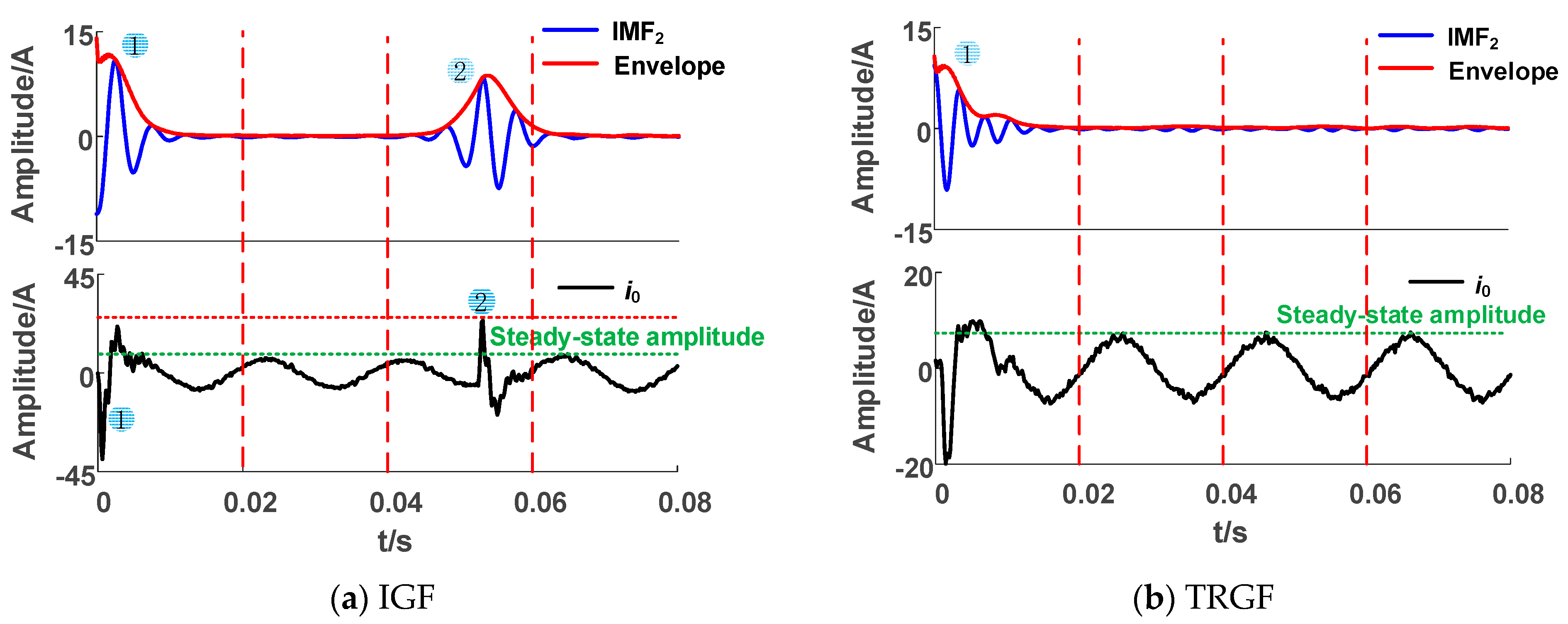
- Fault data: In actual distribution networks, most of the collected single line-to-ground fault data are recorded as SLGFs. These faults are not recognized as transition resistance grounding faults (TRGFs), arc grounding faults (AGFs), intermittent grounding faults (IGFs), transient grounding faults (TGFs), etc. Moreover, some faults, such as TGFs, may not require protection actions. Thus, it is difficult to obtain realistic recorded data containing multiple types of SLGFs.
- (1)
- Multi-type fault classification: We utilize six types of SLGFs in the actual distribution network to identify and classify the specific type of grounding fault, which is conducive to further determining the causes of grounding faults in the distribution network and formulating targeted measures for hidden danger management and fault elimination.
- (2)
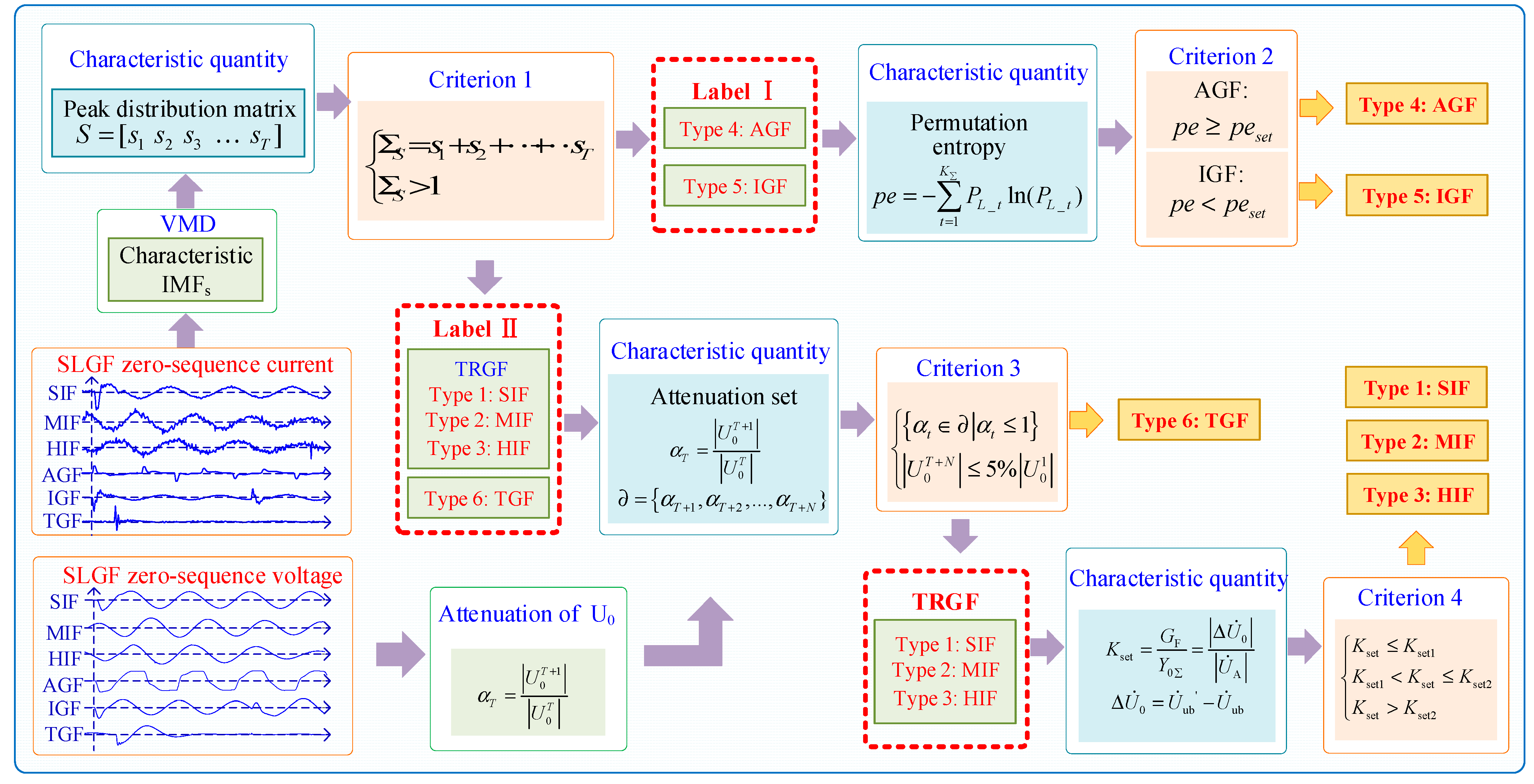
- Multilevel method: We construct a decision-tree-based multilevel strategy for fault type classification. By grouping the same features and distinguishing different features, four criteria are obtained based on the feature analysis of different fault types. Moreover, a multilevel progressive classification method for the SLGFs is carried out.
- (3)
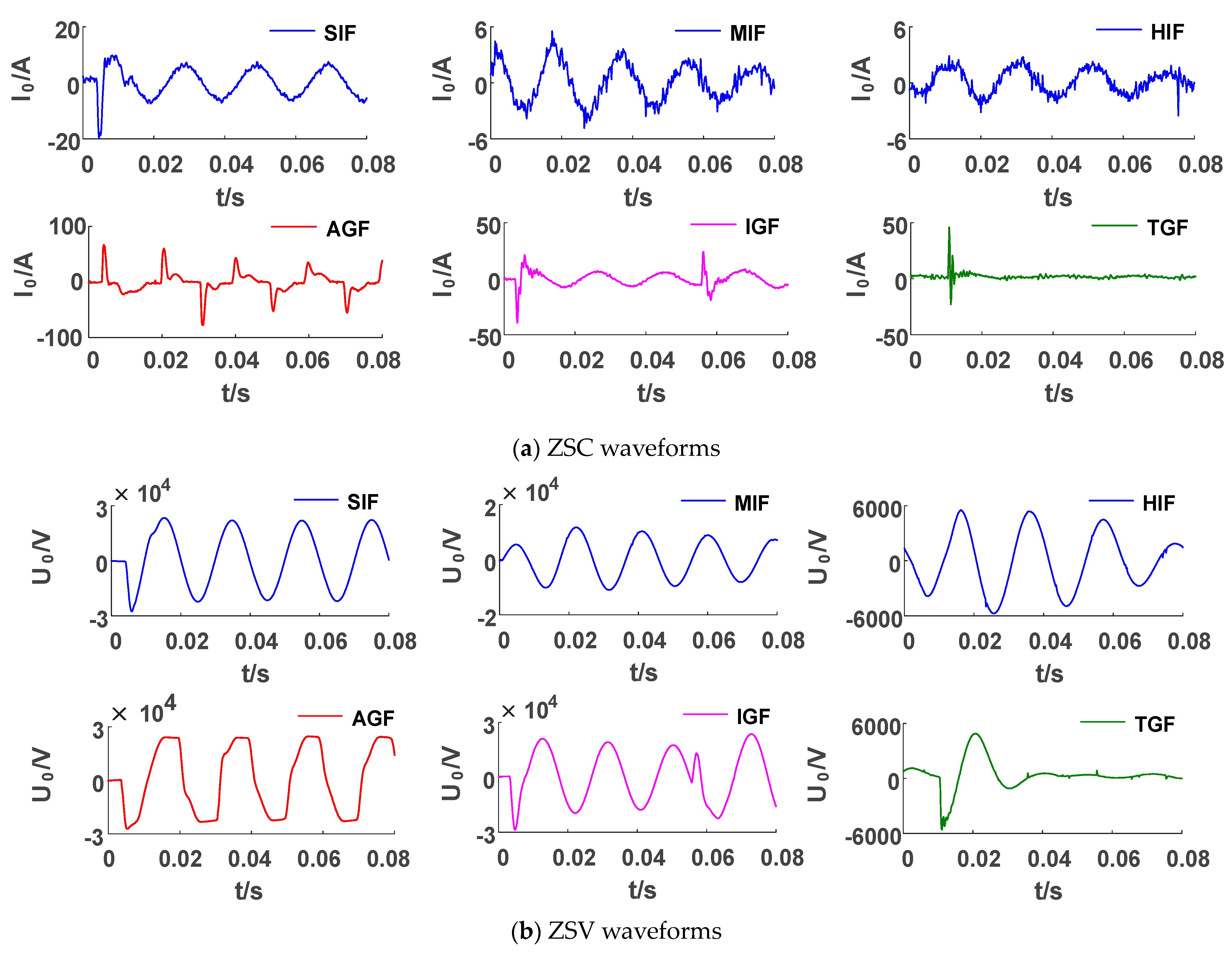
- Realistic recorded waveforms: The data verified in this paper are the actual single line-to-ground fault (SLGF) data in China’s distribution network, which include six types: small-impedance faults (SIFs), medium-impedance faults (MIFs), high-impedance faults (HIFs), arc grounding faults (AGFs), intermittent grounding faults (IGFs), and transient grounding faults (TGFs). The verification of the actual fault data reflects the engineering applicability of the method.
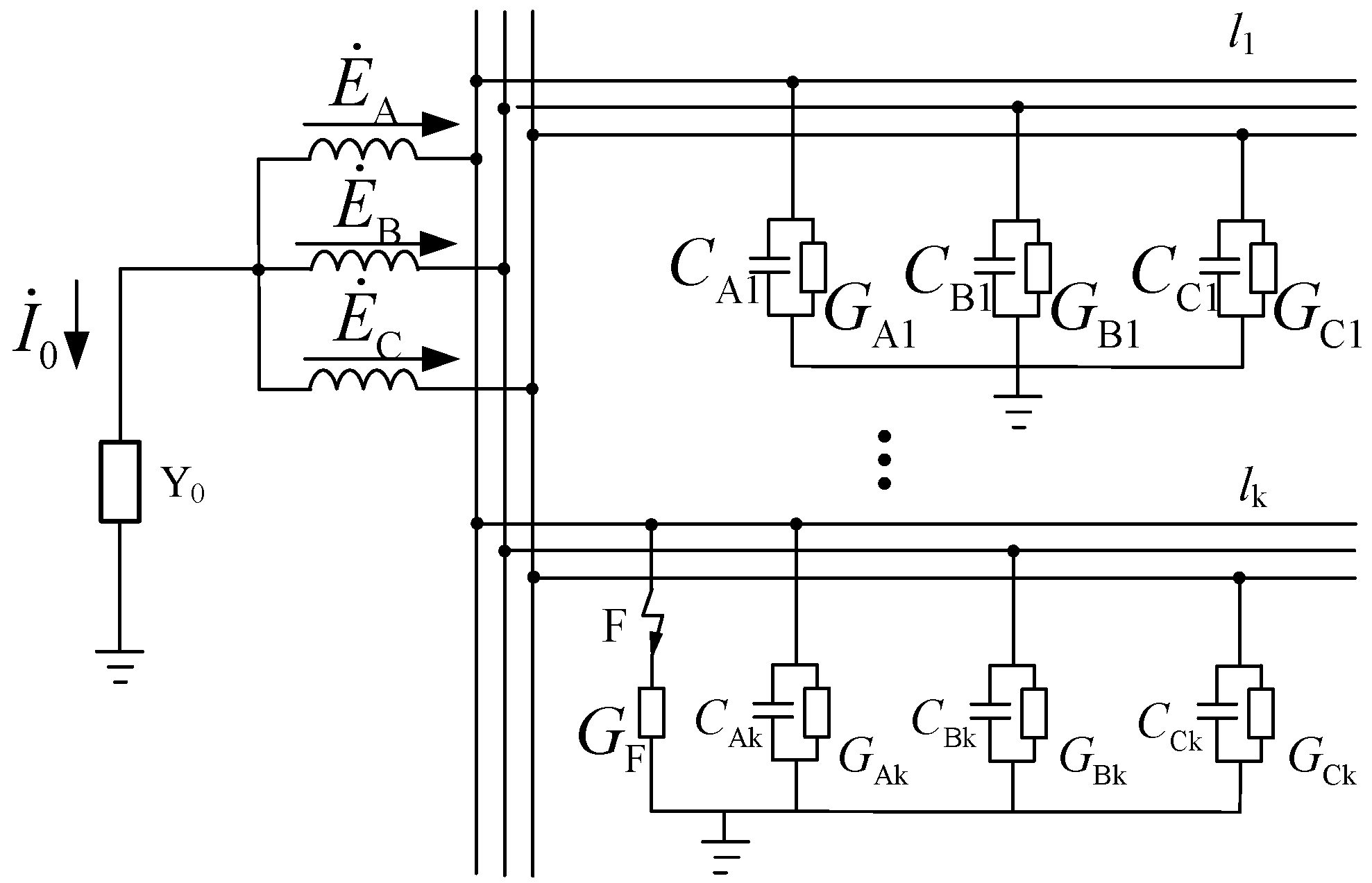
2. Fault Transition Conductance Analysis
3. Multilevel Classification Method
3.1. Criterion 1
3.2. Criterion 2
3.3. Criterion 3
3.4. Criterion 4
3.5. Multi-Type Fault Classification Method
4. Simulation and Test Verification
4.1. Different Fault Condition Test
4.2. Unbalanced Load Test
5. Practical Fault Data Verification
6. Adaptability Analysis
6.1. Noise Test
6.2. Data Loss Test
7. Conclusions
- (1)
- By deducing the generation mechanism of the zero sequence voltage, we obtained the relationship between the transition conductance, the in ZSV, and the fault phase voltage: the transition conductance is positively correlated with the variation in ZSV and inversely correlated with the fault phase voltage.
- (2)
- After we analyzed and compared the characteristics of various SLGFs, we obtained inductive criteria for the same features and discrimination criteria for different features. Using four criteria to construct a multi-level classification method, the waveforms under different fault conditions were verified, and the results showed that the proposed method has high reliability.
- (3)
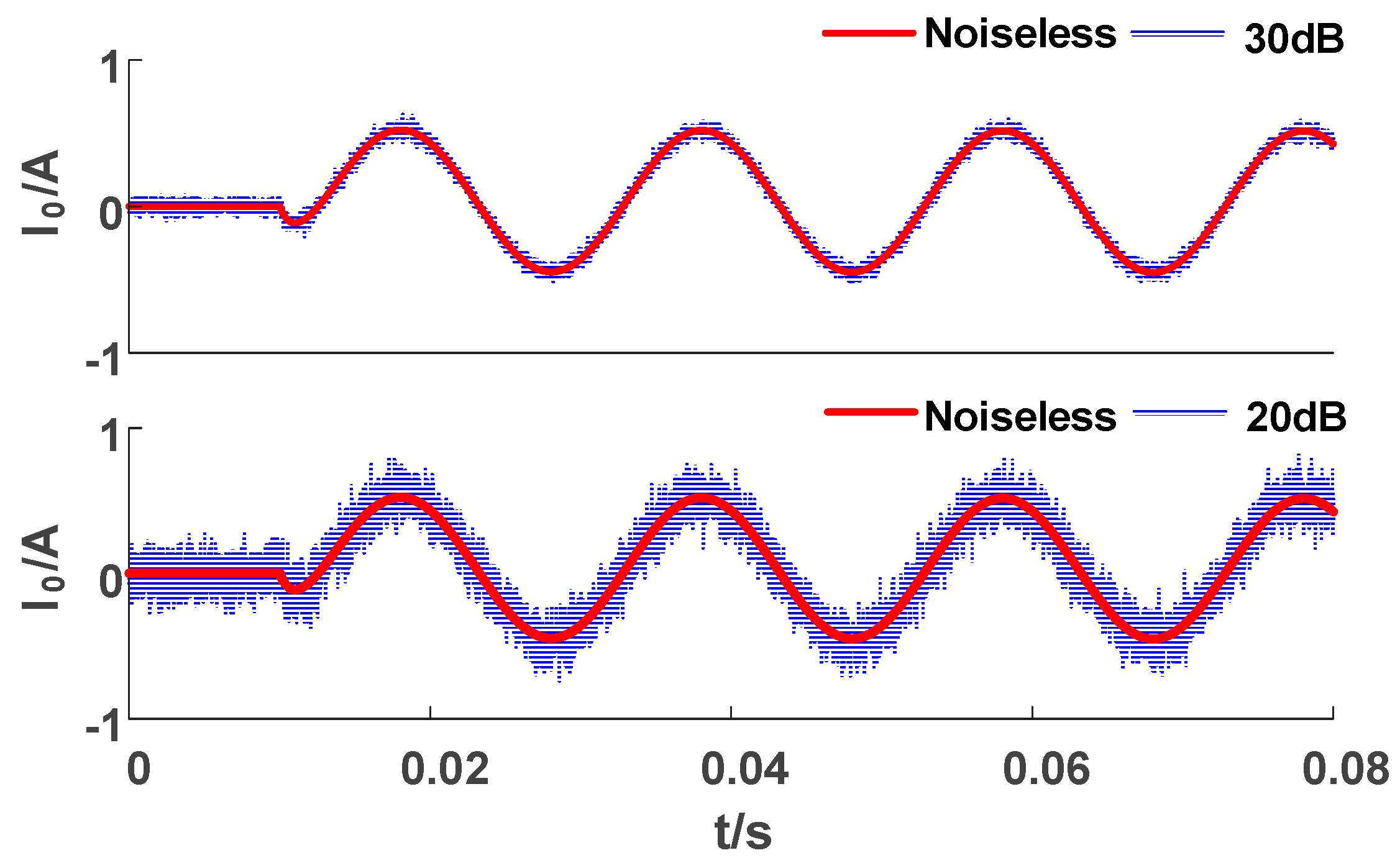
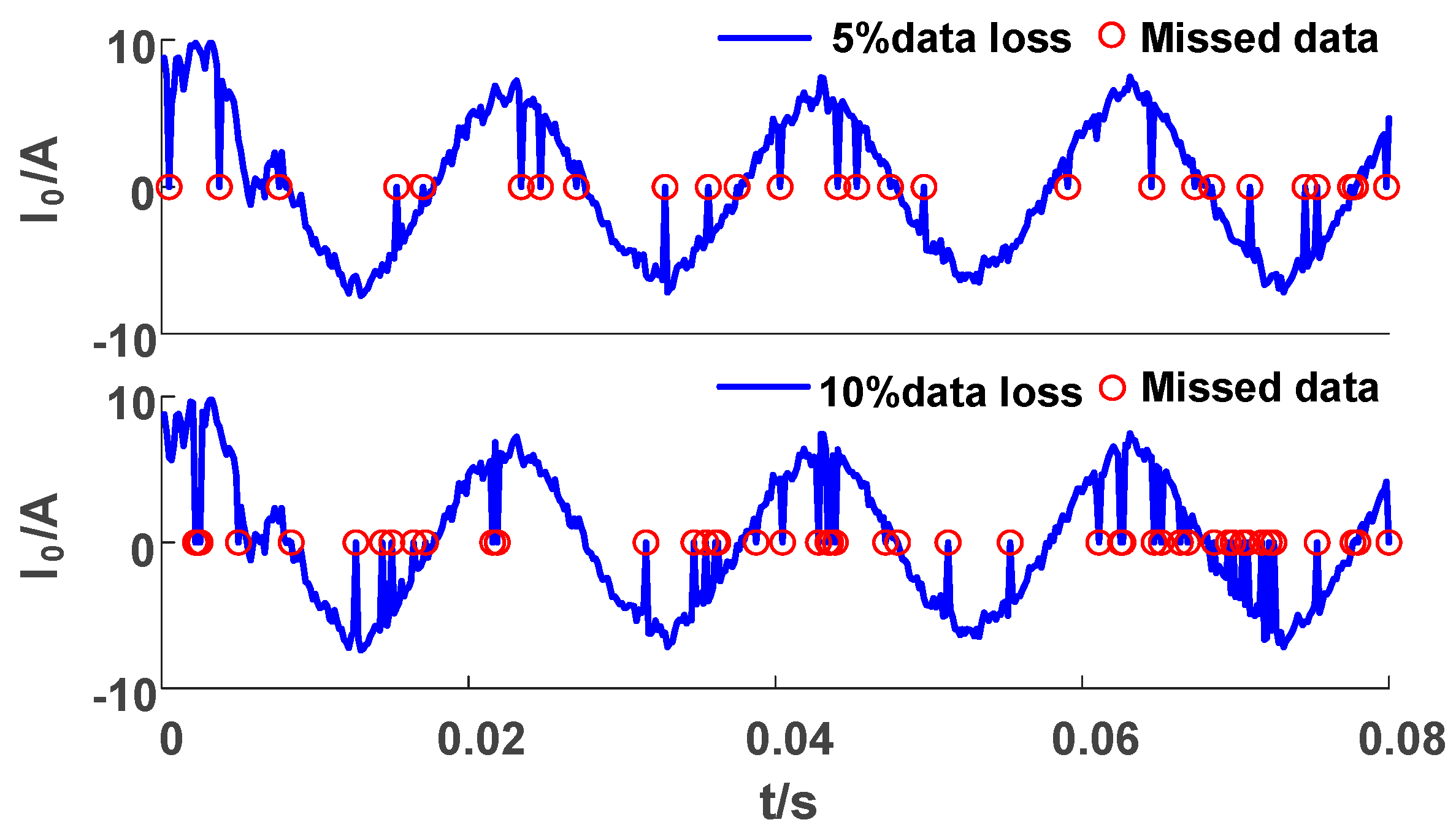
- The proposed method judged faults correctly for both balanced and unbalanced topology models. Moreover, the method has good robustness under interference conditions, such as noise effects and data loss. In addition, the validation of actual fault data indicates that the method has certain engineering applicability.
Author Contributions
Funding
Institutional Review Board Statement
Informed Consent Statement
Data Availability Statement
Conflicts of Interest
Abbreviations
| SLGF | Single line-to-ground fault |
| ZSV | Zero sequence voltage |
| WT | Wavelet transform |
| ZSC | Zero sequence current |
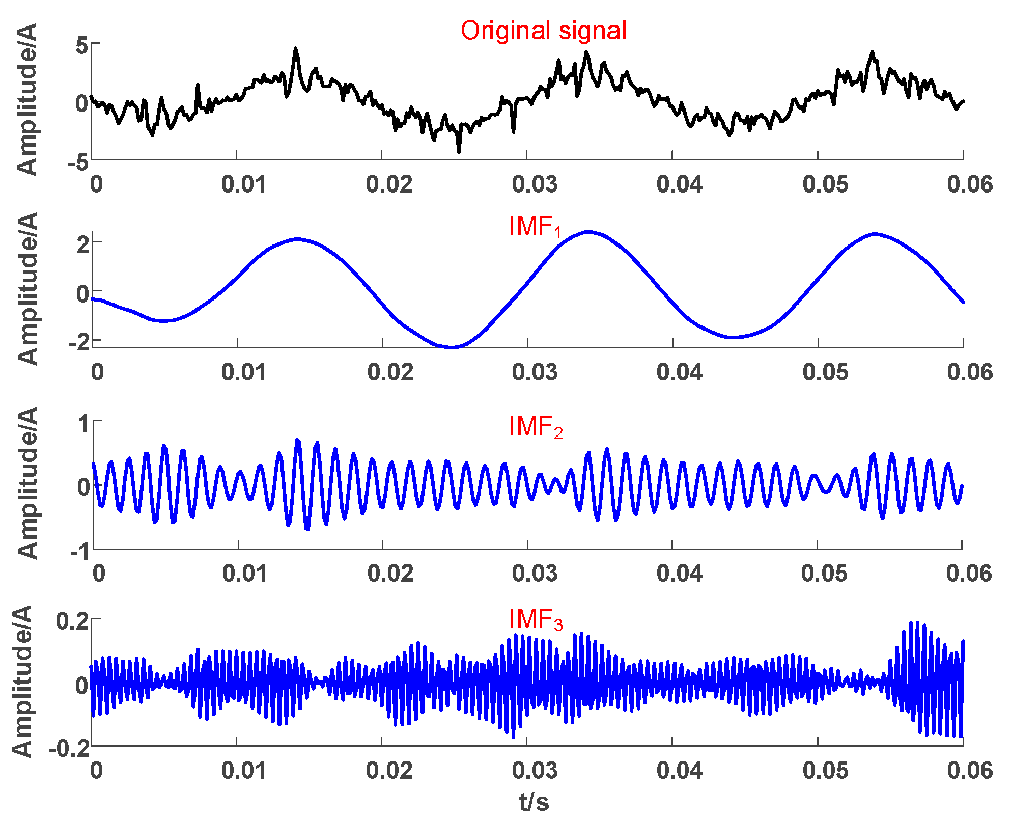
| VMD | Variational mode decomposition |
| EMD | Empirical mode decomposition |
| CEEMDAN | Complete ensemble empirical mode decomposition with adaptive noise |
| IMF | Intrinsic mode function |
| CNN | Convolutional neural network |
| TRGF | Transition resistance grounding fault |
| SIF | Small-impedance fault |
| MIF | Medium-impedance fault |
| HIF | High-impedance fault |
| AGF | Arc grounding fault |
| IGF | Intermittent grounding fault |
| TGF | Transient grounding fault |
References
- Liu, K.; Zhang, S.; Li, B.; Zhang, C.; Liu, B.; Jin, H.; Zhao, J. Faulty Feeder Identification Based on Data Analysis and Similarity Comparison for Flexible Grounding System in Electric Distribution Networks. Sensors 2021, 21, 154. [Google Scholar] [CrossRef] [PubMed]
- Hou, Z.Q.; Zhang, Z.H.; Wang, Y.Z.; Duan, J.D.; Yan, W.Y.; Lu, W.C. A Single-Phase High-Impedance Ground Faulty Feeder Detection Method for Small Resistance to Ground Systems Based on Current-Voltage Phase Difference. Sensors 2022, 22, 4646. [Google Scholar] [CrossRef] [PubMed]
- Jiang, J.A.; Chuang, C.L.; Wang, Y.C.; Hung, C.H.; Wang, J.Y.; Lee, C.H.; Hsiao, Y.T. A Hybrid Framework for Fault Detection, Classification, and Location-Part I: Concept, Structure, and Methodology. IEEE Trans. Power Deliv. 2011, 26, 1988–1998. [Google Scholar] [CrossRef]
- Ghaderi, A.; Mohammadpour, H.A.; Ginn, H.L.; Shin, Y.J. High-Impedance Fault Detection in the Distribution Network Using the Time-Frequency-Based Algorithm. IEEE Trans. Power Deliv. 2015, 30, 1260–1268. [Google Scholar] [CrossRef]
- Guo, M.-F.; Yang, N.-C. Features-clustering-based earth fault detection using singular-value decomposition and fuzzy c-means in resonant grounding distribution systems. Int. J. Electr. Power Energy Syst. 2017, 93, 97–108. [Google Scholar] [CrossRef]
- Wu, S.-D.; Wu, P.-H.; Wu, C.-W.; Ding, J.-J.; Wang, C.-C. Bearing Fault Diagnosis Based on Multiscale Permutation Entropy and Support Vector Machine. Entropy 2012, 14, 1343–1356. [Google Scholar] [CrossRef]
- Yan, X.A.; Liu, Y.; Xu, Y.D.; Jia, M.P. Multichannel fault diagnosis of wind turbine driving system using multivariate singular spectrum decomposition and improved Kolmogorov complexity. Renew. Energy 2021, 170, 724–748. [Google Scholar] [CrossRef]
- Yan, X.; Jia, M. Bearing fault diagnosis via a parameter-optimized feature mode decomposition. Measurement 2022, 203, 112016. [Google Scholar] [CrossRef]
- Chen, K.; Hu, J.; He, J. Detection and Classification of Transmission Line Faults Based on Unsupervised Feature Learning and Convolutional Sparse Autoencoder. IEEE Trans. Smart Grid 2018, 9, 1748–1758. [Google Scholar] [CrossRef]
- Chen, K.; Hu, J.; He, J. A Framework for Automatically Extracting Overvoltage Features Based on Sparse Autoencoder. IEEE Trans. Smart Grid 2018, 9, 594–604. [Google Scholar] [CrossRef]
- Deng, X.; Yuan, R.; Xiao, Z.; Li, T.; Wang, K.L.L. Fault location in loop distribution network using SVM technology. Int. J. Electr. Power Energy Syst. 2015, 65, 254–261. [Google Scholar] [CrossRef]
- Yi, Z.; Etemadi, A.H. Line-to-Line Fault Detection for Photovoltaic Arrays Based on Multiresolution Signal Decomposition and Two-Stage Support Vector Machine. IEEE Trans. Ind. Electron. 2017, 64, 8546–8556. [Google Scholar] [CrossRef]
- Yu, K.; Zou, H.; Zeng, X.; Li, Y.; Li, H.; Zhuo, C.; Wang, Z. Faulty feeder detection of single phase-earth fault based on fuzzy measure fusion criterion for distribution networks. Int. J. Electr. Power Energy Syst. 2021, 125, 106459. [Google Scholar] [CrossRef]
- Jawad, R.S.; Abid, H. HVDC Fault Detection and Classification with Artificial Neural Network Based on ACO-DWT Method. Energies 2023, 16, 1064. [Google Scholar] [CrossRef]
- Pourahmadi-Nakhli, M.; Safavi, A.A. Path Characteristic Frequency-Based Fault Locating in Radial Distribution Systems Using Wavelets and Neural Networks. IEEE Trans. Power Deliv. 2011, 26, 772–781. [Google Scholar] [CrossRef]
- Jamali, S.; Bahmanyar, A.; Ranjbar, S. Hybrid classifier for fault location in active distribution networks. Prot. Control. Mod. Power Syst. 2020, 5, 17. [Google Scholar] [CrossRef]
- Guo, M.-F.; Yang, N.-C.; Chen, W.-F. Deep-Learning-Based Fault Classification Using Hilbert-Huang Transform and Convolutional Neural Network in Power Distribution Systems. IEEE Sens. J. 2019, 19, 6905–6913. [Google Scholar] [CrossRef]
- Du, Y.; Liu, Y.; Shao, Q.; Luo, L.; Dai, J.; Sheng, G.; Jiang, X. Single Line-to-Ground Faulted Line Detection of Distribution Systems With Resonant Grounding Based on Feature Fusion Framework. IEEE Trans. Power Deliv. 2019, 34, 1766–1775. [Google Scholar] [CrossRef]
- Yang, D.; Pang, Y.; Zhou, B.; Li, K. Fault Diagnosis for Energy Internet Using Correlation Processing-Based Convolutional Neural Networks. IEEE Trans. Syst. Man Cybern.-Syst. 2019, 49, 1739–1748. [Google Scholar] [CrossRef]
- Marin-Quintero, J.; Orozco-Henao, C.; Bretas, A.S.; Velez, J.C.; Herrada, A.; Barranco-Carlos, A.; Percybrooks, W.S. Adaptive Fault Detection Based on Neural Networks and Multiple Sampling Points for Distribution Networks and Microgrids. J. Mod. Power Syst. Clean Energy 2022, 10, 1648–1657. [Google Scholar] [CrossRef]
- Hu, J.; Hu, W.; Chen, J.; Cao, D.; Zhang, Z.; Liu, Z.; Chen, Z.; Blaabjerg, F. Fault Location and Classification for Distribution Systems Based on Deep Graph Learning Methods. J. Mod. Power Syst. Clean Energy 2023, 11, 35–51. [Google Scholar] [CrossRef]
- Zhu, K.; Pong, P.W.T. Fault Classification of Power Distribution Cables by Detecting Decaying DC Components With Magnetic Sensing. IEEE Trans. Instrum. Meas. 2020, 69, 2016–2027. [Google Scholar] [CrossRef]
- Xiao, Q.-M.; Guo, M.-F.; Chen, D.-Y. High-Impedance Fault Detection Method Based on One-Dimensional Variational Prototyping-Encoder for Distribution Networks. IEEE Syst. J. 2022, 16, 966–976. [Google Scholar] [CrossRef]
- Wang, X.; Gao, J.; Wei, X.; Song, G.; Wu, L.; Liu, J.; Zeng, Z.; Kheshti, M. High Impedance Fault Detection Method Based on Variational Mode Decomposition and Teager-Kaiser Energy Operators for Distribution Network. IEEE Trans. Smart Grid 2019, 10, 6041–6054. [Google Scholar] [CrossRef]
- Song, X.; Gao, F.; Chen, Z.; Liu, W. A Negative Selection Algorithm-Based Identification Framework for Distribution Network Faults With High Resistance. IEEE Access 2019, 7, 109363–109374. [Google Scholar] [CrossRef]
- Wang, X.; Song, G.; Gao, J.; Wei, X.; Wei, Y.; Kheshti, M.; Hu, Z.; Zhang, Z. High impedance fault detection method based on improved complete ensemble empirical mode decomposition for DC distribution network. Int. J. Electr. Power Energy Syst. 2019, 107, 538–556. [Google Scholar] [CrossRef]
- Liu, H.; Liu, S.; Zhao, J.; Bi, T.; Yu, X. Dual-Channel Convolutional Network-Based Fault Cause Identification for Active Distribution System Using Realistic Waveform Measurements. IEEE Trans. Smart Grid 2022, 13, 4899–4908. [Google Scholar] [CrossRef]
- Zhang, S.; Zang, T.; Zhang, W.; Xiao, X. Fault Feeder Identification in Non-effectively Grounded Distribution Network with Secondary Earth Fault. J. Mod. Power Syst. Clean Energy 2021, 9, 1137–1148. [Google Scholar] [CrossRef]
- Yuan, J.; Hu, Y.; Liang, Y.; Jiao, Z. Faulty Feeder Detection for Single Line-to-Ground Fault in Distribution Networks With DGs Based on Correlation Analysis and Harmonics Energy. IEEE Trans. Power Deliv. 2023, 38, 1020–1029. [Google Scholar] [CrossRef]
- Achlerkar, P.D.; Samantaray, S.R.; Manikandan, M.S. Variational Mode Decomposition and Decision Tree Based Detection and Classification of Power Quality Disturbances in Grid-Connected Distributed Generation System. IEEE Trans. Smart Grid 2018, 9, 3122–3132. [Google Scholar] [CrossRef]
- Fabila-Carrasco, J.S.; Tan, C.; Escudero, J. Permutation Entropy for Graph Signals. IEEE Trans. Signal Inf. Process. Netw. 2022, 8, 288–300. [Google Scholar] [CrossRef]
- Wei, X.; Wang, X.; Gao, J.; Yang, D.; Wei, K.; Guo, L.; Wei, Y. Faulty Feeder Identification Method Considering Inverter Transformer Effects in Converter Dominated Distribution Network. IEEE Trans. Smart Grid 2023, 14, 939–953. [Google Scholar] [CrossRef]
- Long, Y.; Zhao, F.; Zheng, M.; Jin, G.; Zhang, H.; Wang, R. A Novel Azimuth Ambiguity Suppression Method for Spaceborne Dual-Channel SAR-GMTI. IEEE Geosci. Remote Sens. Lett. 2021, 18, 87–91. [Google Scholar] [CrossRef]
- Kang, M.-S.; Baek, J.-M. Efficient SAR Imaging Integrated With Autofocus via Compressive Sensing. IEEE Geosci. Remote Sens. Lett. 2022, 19, 4514905. [Google Scholar] [CrossRef]
- Long, Y.; Zhao, F.; Zheng, M.; Jin, G.; Zhang, H. An Azimuth Ambiguity Suppression Method Based on Local Azimuth Ambiguity-to-Signal Ratio Estimation. IEEE Geosci. Remote Sens. Lett. 2020, 17, 2075–2079. [Google Scholar] [CrossRef]
- Kang, M.S.; Baek, J.M. SAR Image Reconstruction via Incremental Imaging With Compressive Sensing. IEEE Trans. Aerosp. Electron. Syst. 2023, 59, 4450–4463. [Google Scholar] [CrossRef]


| Feeder Types | Phase Sequence | R (Ω/km) | L (mH/km) | C (μF/km) |
|---|---|---|---|---|
| Overhead feeder | Positive sequence | 0.1700 | 1.2000 | 0.0097 |
| Zero sequence | 0.2300 | 5.4800 | 0.0060 | |
| Cable feeder | Positive sequence | 0.1930 | 0.4420 | 0.1430 |
| Zero sequence | 1.9300 | 5.4800 | 0.1430 |
| Type | Parameter Value |
|---|---|
| Fault feeder | l1, l3, l4 |
| Transition resistance/Ω | 0.01, 5, 10; 50, 60, 70, 500, 1000, 1500 |
| Arc fault model | Emanuel |
| Interval time of IGF/s | 0.02, 0.04, 0.06 |
| Time of TGF/s | 0.01, 0.02, 0.03 |
| Type | Fault Feeder | Fault Parameters | Peak Matrix | Number of Peak | Label |
|---|---|---|---|---|---|
| AGF | l1 | - | [2 0 0 0] | 2 > 1 | Ⅰ |
| l3 | - | [2 0 0 0] | 2 > 1 | ||
| l4 | - | [2 0 0 0] | 2 > 1 | ||
| IGF | l1 | 0.02 s | [1 0 1 0] | 2 > 1 | |
| l3 | 0.04 s | [1 0 1 0] | 2 > 1 | ||
| l4 | 0.06 s | [1 0 0 1] | 2 > 1 | ||
| TGF | l1 | 0.01 s | [1 0 0 0] | 1 ≯ 1 | Ⅱ |
| l3 | 0.02 s | [1 0 0 0] | 1 ≯ 1 | ||
| l4 | 0.03 s | [1 0 0 0] | 1 ≯ 1 | ||
| SIF | l1 | 0.01 Ω | [1 0 0 0] | 1 ≯ 1 | |
| l3 | 5 Ω | [1 0 0 0] | 1 ≯ 1 | ||
| l4 | 10 Ω | [1 0 0 0] | 1 ≯ 1 | ||
| MIF | l1 | 50 Ω | [1 0 0 0] | 1 ≯ 1 | |
| l3 | 60 Ω | [1 0 0 0] | 1 ≯ 1 | ||
| l4 | 70 Ω | [1 0 0 0] | 1 ≯ 1 | ||
| HIF | l1 | 500 Ω | [1 0 0 0] | 1 ≯ 1 | |
| l3 | 1000 Ω | [1 0 0 0] | 1 ≯ 1 | ||
| l4 | 1500 Ω | [1 0 0 0] | 1 ≯ 1 |
| Type | Fault Feeder | Fault Parameters | pe | Type | Result |
|---|---|---|---|---|---|
| AGF | l1 | - | 0.9861 | 4 | AGF |
| l3 | - | 0.9884 | 4 | AGF | |
| l4 | - | 0.9807 | 4 | AGF | |
| IGF | l1 | 0.02 s | 0.5473 | 5 | IGF |
| l3 | 0.04 s | 0.5182 | 5 | IGF | |
| l4 | 0.06 s | 0.3851 | 5 | IGF |
| Type | Fault Feeder | Parameters | Result | ||
|---|---|---|---|---|---|
| TGF | l1 | 0.01 s | [0.20 0.53 0.53 0.54] | 0.14 | TGF |
| l3 | 0.02 s | [0.18 0.15 0.53 0.53] | 0.04 | TGF | |
| l4 | 0.03 s | [0.70 1.17 0.53 0.53] | 0.22 | TGF | |
| SIF | l1 | 0.01 Ω | [1.02 1.00 1.00 1.00] | 15.63 | TRGF |
| l3 | 5 Ω | [1.02 1.00 1.00 1.00] | 8.63 | ||
| l4 | 10 Ω | [1.00 1.00 1.00 1.00] | 9.36 | ||
| MIF | l1 | 50 Ω | [1.01 1.00 1.00 1.00] | 3.50 | |
| l3 | 60 Ω | [1.01 1.00 1.00 1.00] | 2.60 | ||
| l4 | 70 Ω | [1.00 1.00 1.00 1.00] | 2.65 | ||
| HIF | l1 | 500 Ω | [1.00 1.00 1.00 1.00] | 0.43 | |
| l3 | 1000 Ω | [0.99 1.00 1.00 1.00] | 0.20 | ||
| l4 | 1500 Ω | [0.99 1.00 1.00 1.00] | 0.15 |
| Type | Fault Feeder | Fault Parameters | Type | Result | |
|---|---|---|---|---|---|
| SIF | l1 | 0.01 Ω | 9.6632 | 1 | SIF |
| l3 | 5 Ω | 2.5855 | 1 | SIF | |
| l4 | 10 Ω | 3.1688 | 1 | SIF | |
| MIF | l1 | 50 Ω | 0.7096 | 2 | MIF |
| l3 | 60 Ω | 0.4960 | 2 | MIF | |
| l4 | 70 Ω | 0.5105 | 2 | MIF | |
| HIF | l1 | 500 Ω | 0.0727 | 3 | HIF |
| l3 | 1000 Ω | 0.0330 | 3 | HIF | |
| l4 | 1500 Ω | 0.0242 | 3 | HIF |
| Type | Fault Location | Fault Parameters | Peak Matrix | Number of Peaks | Label |
|---|---|---|---|---|---|
| AGF | 633 | - | [2 0 0 0] | 2 > 1 | Ⅰ |
| 692 | - | [2 0 0 0] | 2 > 1 | ||
| IGF | 633 | 0.02 s | [1 1 0 0] | 2 > 1 | |
| 692 | 0.04 s | [1 0 1 0] | 2 > 1 | ||
| TGF | 633 | 0.01 s | [1 0 0 0] | 1 ≯ 1 | Ⅱ |
| 692 | 0.03 s | [1 0 0 0] | 1 ≯ 1 | ||
| SIF | 633 | 0.01 Ω | [1 0 0 0] | 1 ≯ 1 | |
| 692 | 5 Ω | [1 0 0 0] | 1 ≯ 1 | ||
| MIF | 633 | 50 Ω | [1 0 0 0] | 1 ≯ 1 | |
| 692 | 60 Ω | [1 0 0 0] | 1 ≯ 1 | ||
| HIF | 633 | 500 Ω | [1 0 0 0] | 1 ≯ 1 | |
| 692 | 1000 Ω | [1 0 0 0] | 1 ≯ 1 |
| Type | Fault Location | Fault Parameters | pe | Type | Result |
|---|---|---|---|---|---|
| AGF | 633 | - | 0.8202 | 4 | AGF |
| 692 | - | 0.8633 | 4 | AGF | |
| IGF | 633 | 0.02 s | 0.4340 | 5 | IGF |
| 692 | 0.04 s | 0.4375 | 5 | IGF |
| Type | Fault Location | Result | ||
|---|---|---|---|---|
| TGF | 633 | [0.58 0.99 1.13 1.07] | = 0.2147 | TGF |
| 692 | [0.40 0.64 1.22 1.08] | = 0.1285 | TGF | |
| SIF | 633 | [1.03 1.00 1.01 1.02] | = 3.1642 | TRGF |
| 692 | [1.04 1.00 1.07 1.06] | = 0.3523 | ||
| MIF | 633 | [1.01 1.00 1.11 1.06] | = 0.2697 | |
| 692 | [1.01 1.00 1.16 1.07] | = 0.1206 | ||
| HIF | 633 | [1.00 1.00 1.13 1.06] | = 0.2454 | |
| 692 | [1.00 1.00 1.20 1.08] | = 0.1001 |
| Type | Fault Feeder | Fault Parameters | Type | Result | |
|---|---|---|---|---|---|
| SIF | l1 | 0.01 Ω | 4.3610 | 1 | SIF |
| l4 | 10 Ω | 0.1095 | 1 | SIF | |
| MIF | l1 | 50 Ω | 0.0125 | 2 | MIF |
| l4 | 70 Ω | 0.0097 | 2 | MIF | |
| HIF | l1 | 200 Ω | 0.0013 | 3 | HIF |
| l4 | 1000 Ω | 0.0006 | 3 | HIF |
| Type | Peak Matrix | pe | Result | Correct? | ||||
|---|---|---|---|---|---|---|---|---|
| AGF | [2 2 2 2] | 0.9136 | - | - | - | - | 4 → AGF | √ |
| [1 2 1 2] | 0.9467 | - | - | - | - | 4 → AGF | √ | |
| [1 2 2 2] | 0.9060 | - | - | - | - | 4 → AGF | √ | |
| IGF | [1 0 1 0] | 0.7826 | - | - | - | - | 5 → IGF | √ |
| [1 0 1 0] | 0.7268 | - | - | - | - | 5 → IGF | √ | |
| [1 0 0 1] | 0.7446 | - | - | - | - | 5 → IGF | √ | |
| TGF | [1 0 0 0] | - | [0.19 0.47 1.06 1.05] | = 272.40 | - | 6 → TGF | √ | |
| [1 0 0 0] | - | [0.19 0.78 1.00 1.02] | = 301.30 | - | 6 → TGF | √ | ||
| [1 0 0 0] | - | [0.90 0.43 1.00 1.07] | = 350.56 | - | 6 → TGF | √ | ||
| SIF | [1 0 0 0] | - | [0.92 1.00 1.02 1.00] | = 15,413.06 | 10.01 | 1 → SIF | √ | |
| [1 0 0 0] | - | [0.99 1.02 1.01 1.00] | = 15,532.50 | 11.95 | 1 → SIF | √ | ||
| [1 0 0 0] | - | [0.94 0.99 0.96 0.94] | = 16,647.74 | 7.55 | 1 → SIF | √ | ||
| MIF | [1 0 0 0] | - | [0.97 0.87 0.85 0.77] | = 4199.69 | 1.94 | 2 → MIF | √ | |
| [1 0 0 0] | - | [0.92 1.02 0.99 0.99] | = 10,026.04 | 1.79 | 2 → MIF | √ | ||
| [1 0 0 0] | - | [0.93 1.02 1.00 0.99] | = 10,102.80 | 1.77 | 2 → MIF | √ | ||
| HIF | [1 0 0 0] | - | [1.02 0.83 0.50 0.50] | = 767.51 | 0.50 | 3 → HIF | √ | |
| [1 0 0 0] | - | [0.94 0.93 0.92 0.87] | = 882.50 | 0.86 | 3 → HIF | √ | ||
| [1 0 0 0] | - | [0.93 0.91 0.86 0.27] | = 514.25 | 0.81 | 3 → HIF | √ |
| Type | Peak Matrix | pe | Result | Correct? | ||||
|---|---|---|---|---|---|---|---|---|
| AGF | [2 2 2 2] | 0.9118 | - | - | - | - | 4 → AGF | √ |
| IGF | [1 0 1 0] | 0.7412 | - | - | - | - | 5 → IGF | √ |
| TGF | [1 0 0 0] | - | [0.19 0.47 1.06 1.05] | = 272.40 | - | 6 → TGF | √ | |
| SIF | [1 0 0 0] | - | [0.92 1.00 1.02 1.00] | = 15,403.64 | 10.01 | 1 → SIF | √ | |
| MIF | [1 0 0 0] | - | [0.97 0.87 0.85 0.77] | = 4199.67 | 1.94 | 2 → MIF | √ | |
| HIF | [1 0 0 0] | - | [1.02 0.83 0.50 0.50] | = 767.51 | 0.50 | 3 → HIF | √ |
| Type | Peak Matrix | pe | Result | Correct? | ||||
|---|---|---|---|---|---|---|---|---|
| AGF | [2 2 2 2] | 0.9369 | - | - | - | - | 4 → AGF | √ |
| IGF | [1 0 1 0] | 0.8170 | - | - | - | - | 5 → IGF | √ |
| TGF | [1 0 0 0] | - | [0.18 0.47 1.07 1.05] | = 261.97 | - | 6 → TGF | √ | |
| SIF | [1 0 0 0] | - | [0.93 0.99 1.01 1.02] | = 14,955.07 | 10.01 | 1 → SIF | √ | |
| MIF | [1 0 0 0] | - | [0.97 0.88 0.85 0.78] | = 4116.56 | 1.94 | 2 → MIF | √ | |
| HIF | [1 0 0 0] | - | [1.02 0.82 0.51 0.50] | = 753.20 | 0.50 | 3 → HIF | √ |
Disclaimer/Publisher’s Note: The statements, opinions and data contained in all publications are solely those of the individual author(s) and contributor(s) and not of MDPI and/or the editor(s). MDPI and/or the editor(s) disclaim responsibility for any injury to people or property resulting from any ideas, methods, instructions or products referred to in the content. |
© 2023 by the authors. Licensee MDPI, Basel, Switzerland. This article is an open access article distributed under the terms and conditions of the Creative Commons Attribution (CC BY) license (https://creativecommons.org/licenses/by/4.0/).
Share and Cite
Liu, J.; Li, C.; Liu, Y.; Sun, J.; Lin, H. Single Line-to-Ground Fault Type Multilevel Classification in Distribution Network Using Realistic Recorded Waveform. Sensors 2023, 23, 8948. https://doi.org/10.3390/s23218948
Liu J, Li C, Liu Y, Sun J, Lin H. Single Line-to-Ground Fault Type Multilevel Classification in Distribution Network Using Realistic Recorded Waveform. Sensors. 2023; 23(21):8948. https://doi.org/10.3390/s23218948
Chicago/Turabian StyleLiu, Jiajun, Chenjing Li, Yue Liu, Ji Sun, and Haokun Lin. 2023. "Single Line-to-Ground Fault Type Multilevel Classification in Distribution Network Using Realistic Recorded Waveform" Sensors 23, no. 21: 8948. https://doi.org/10.3390/s23218948
APA StyleLiu, J., Li, C., Liu, Y., Sun, J., & Lin, H. (2023). Single Line-to-Ground Fault Type Multilevel Classification in Distribution Network Using Realistic Recorded Waveform. Sensors, 23(21), 8948. https://doi.org/10.3390/s23218948