
Guided Direct Time-of-Flight Lidar Using Stereo Cameras for Enhanced Laser Power Efficiency

Abstract
1. Introduction
2. Related Work
2.1. 3D Stacked DToF Sensors
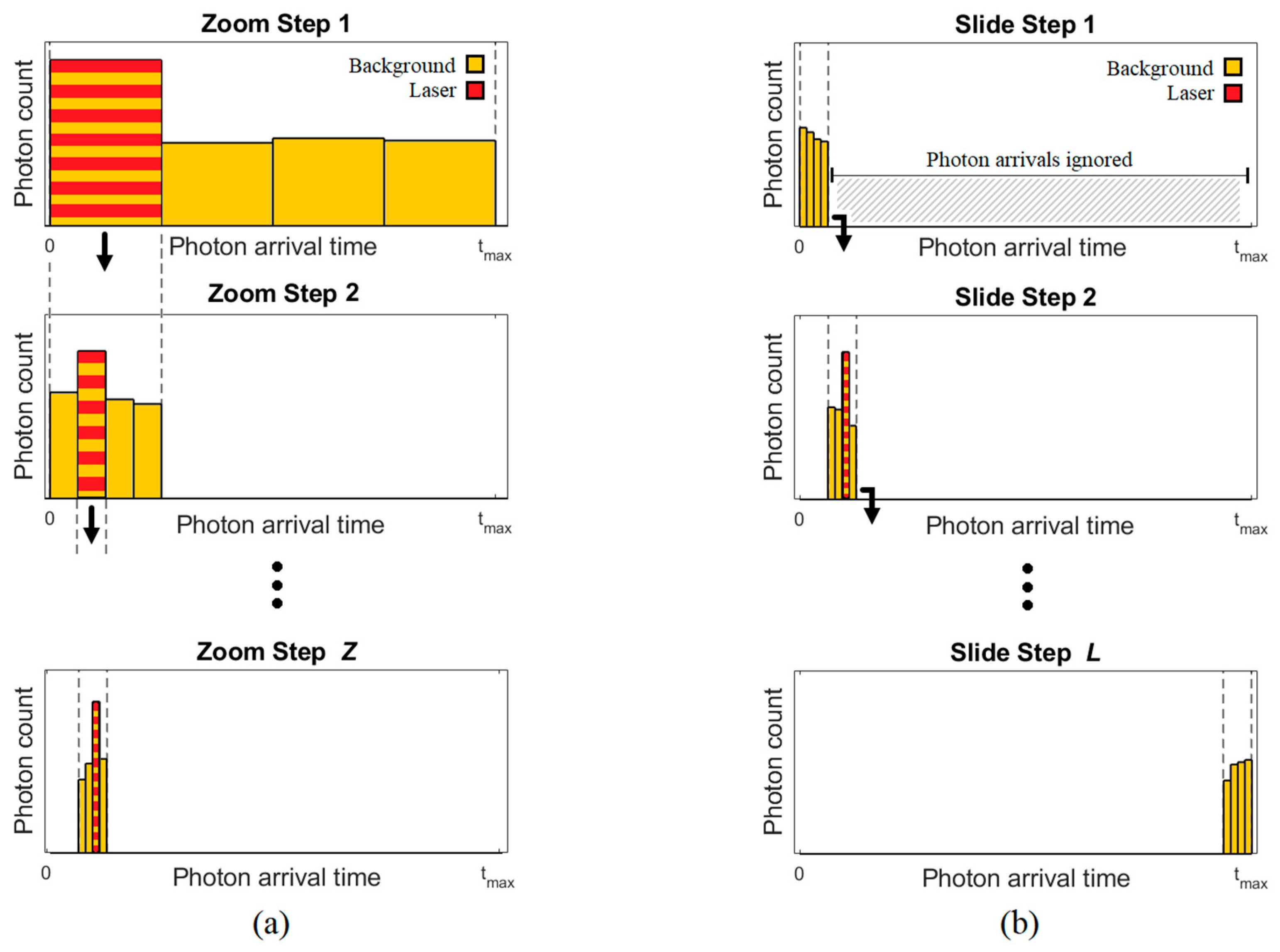
2.2. Partial Histogram DToF Sensors
2.3. Summary of DToF Histogram Approaches
3. Materials & Methods
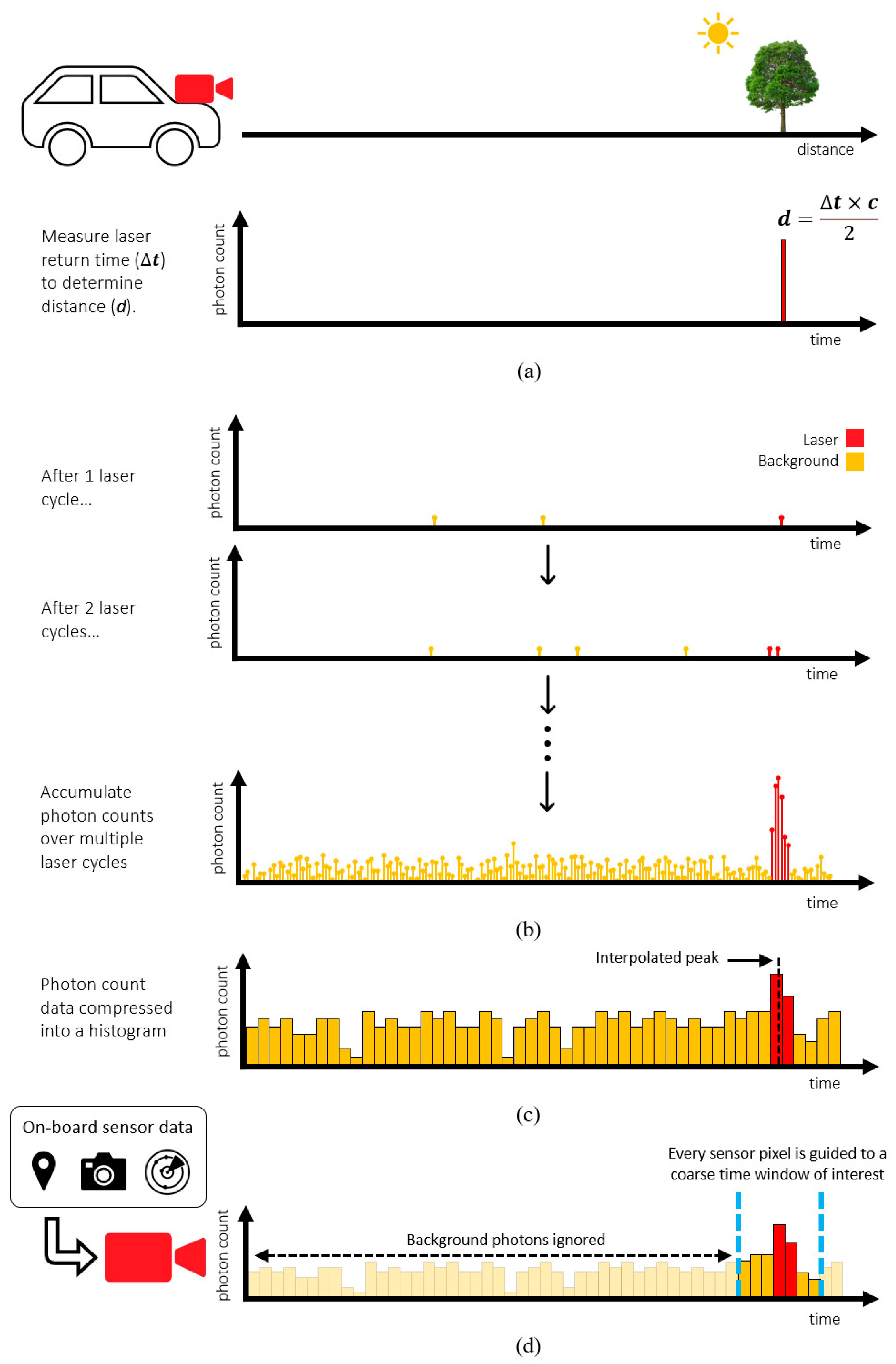
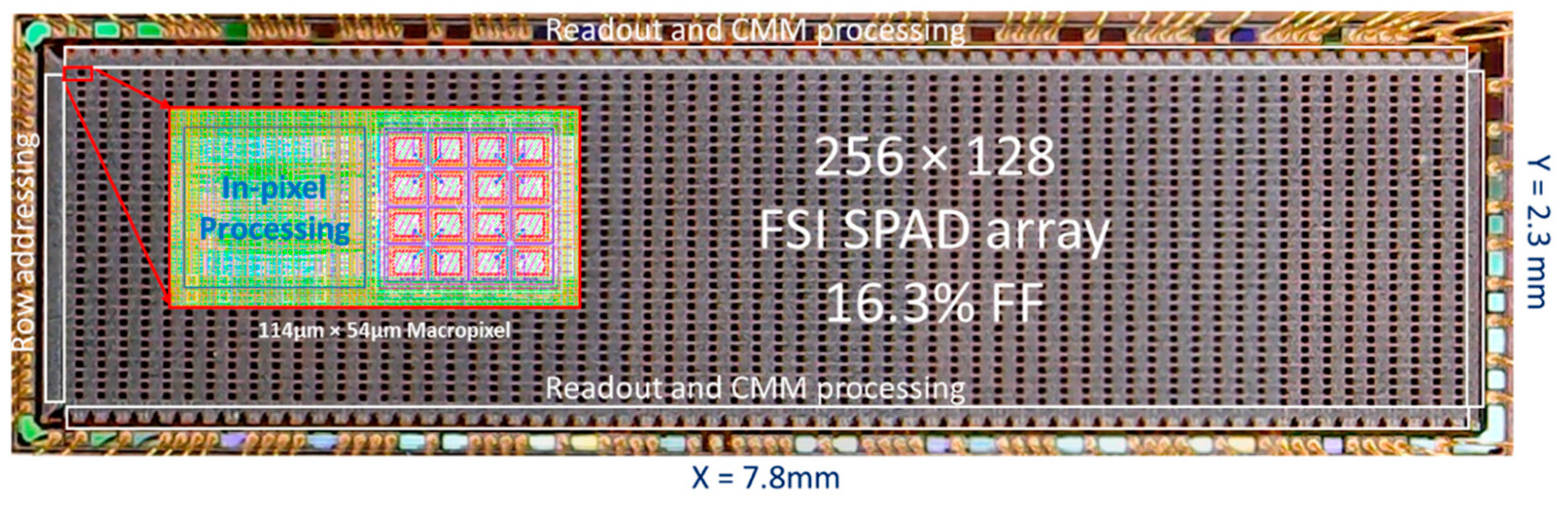
3.1. Guided Lidar Sensor
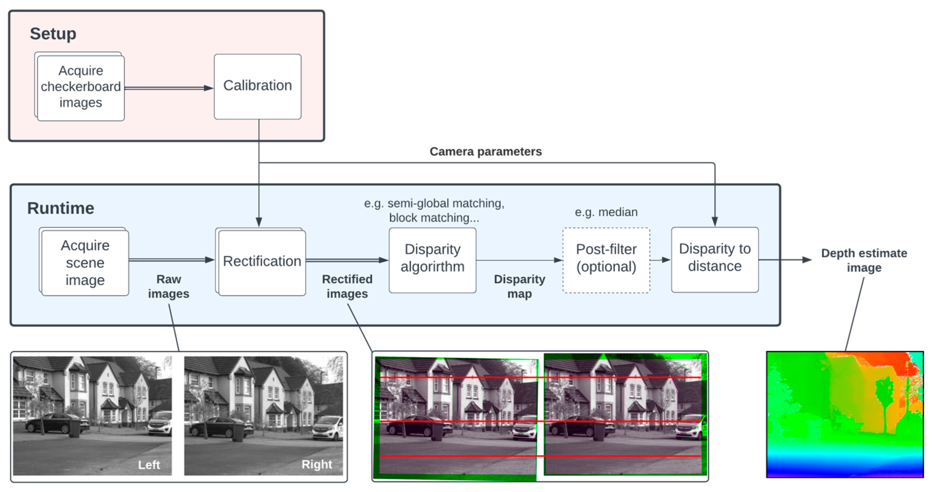
3.2. Guiding Source: Stereo Camera Vision
3.3. Pixel Mapping
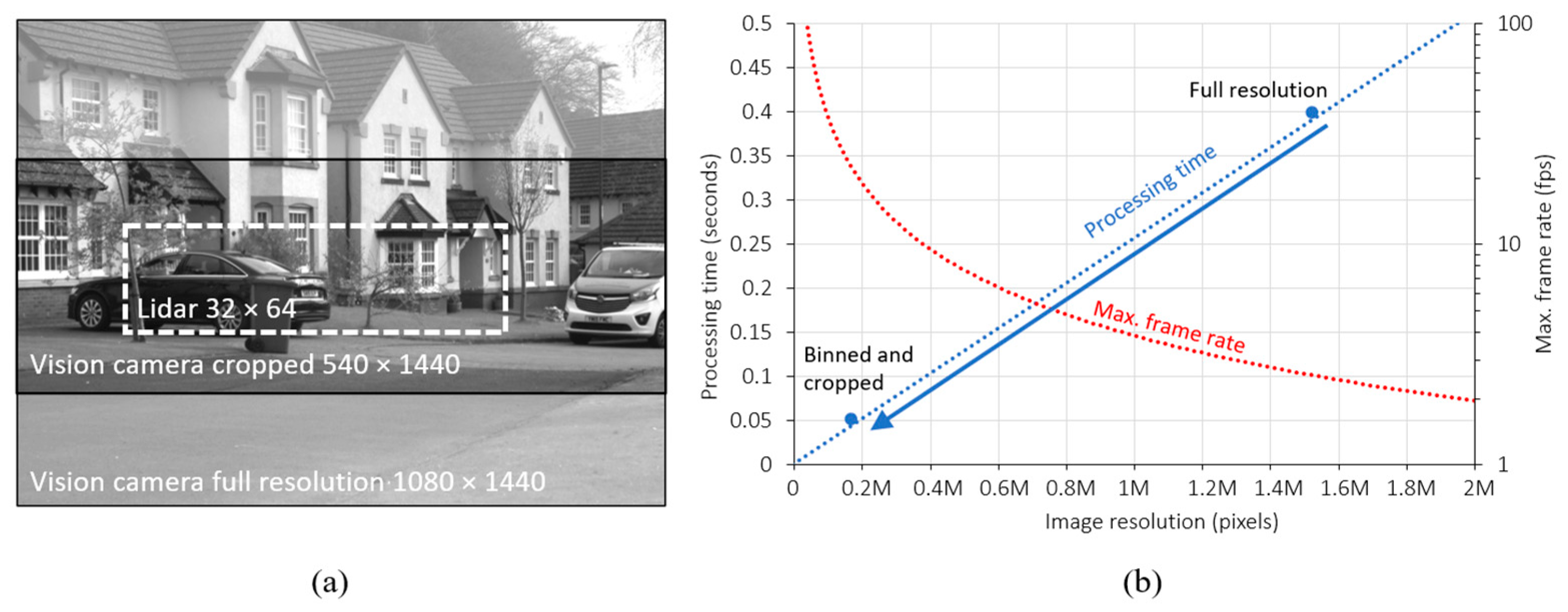
3.4. Process Optimization
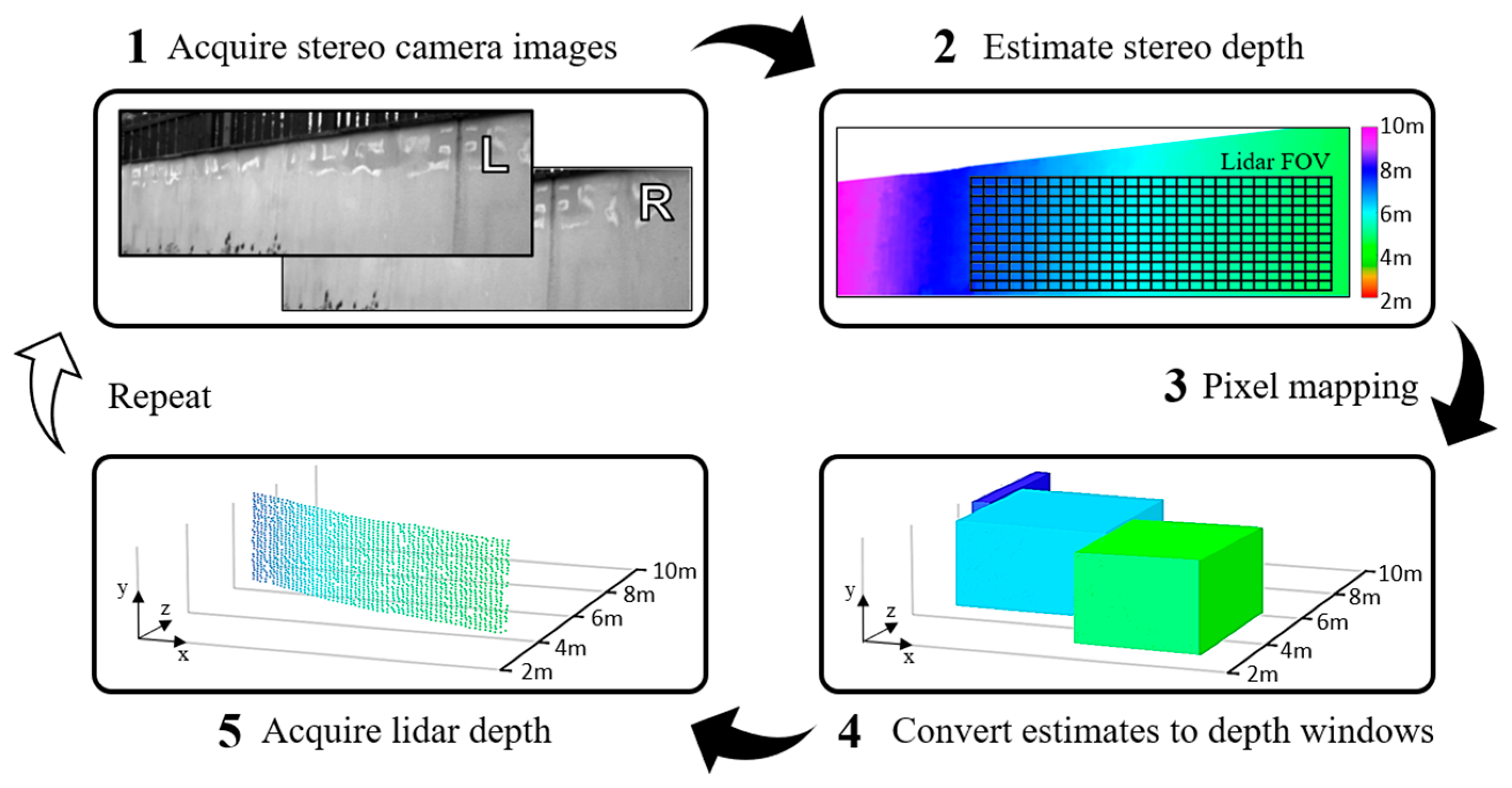
3.5. Process Flow
3.6. Software
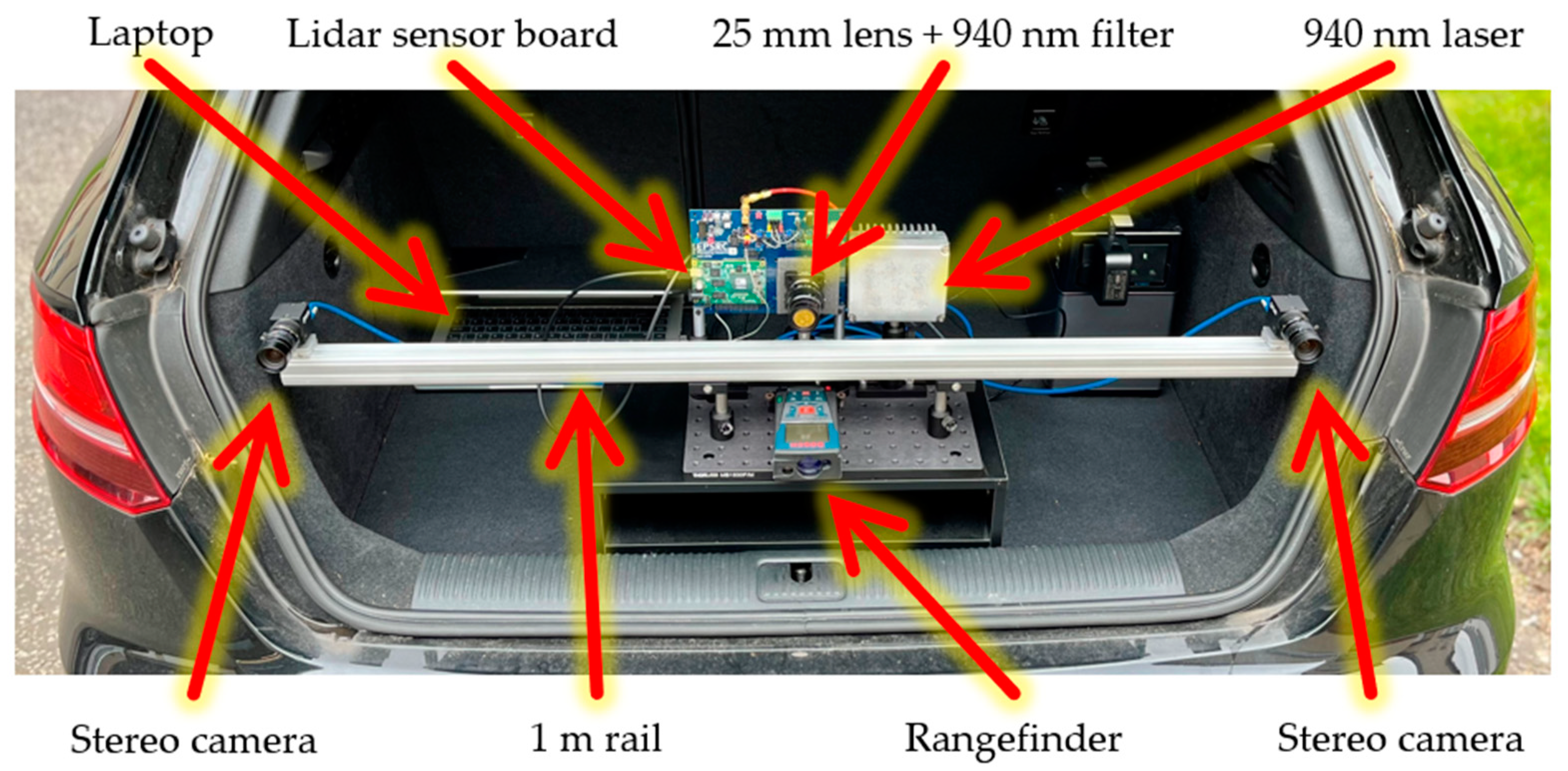
3.7. Setup
4. Results
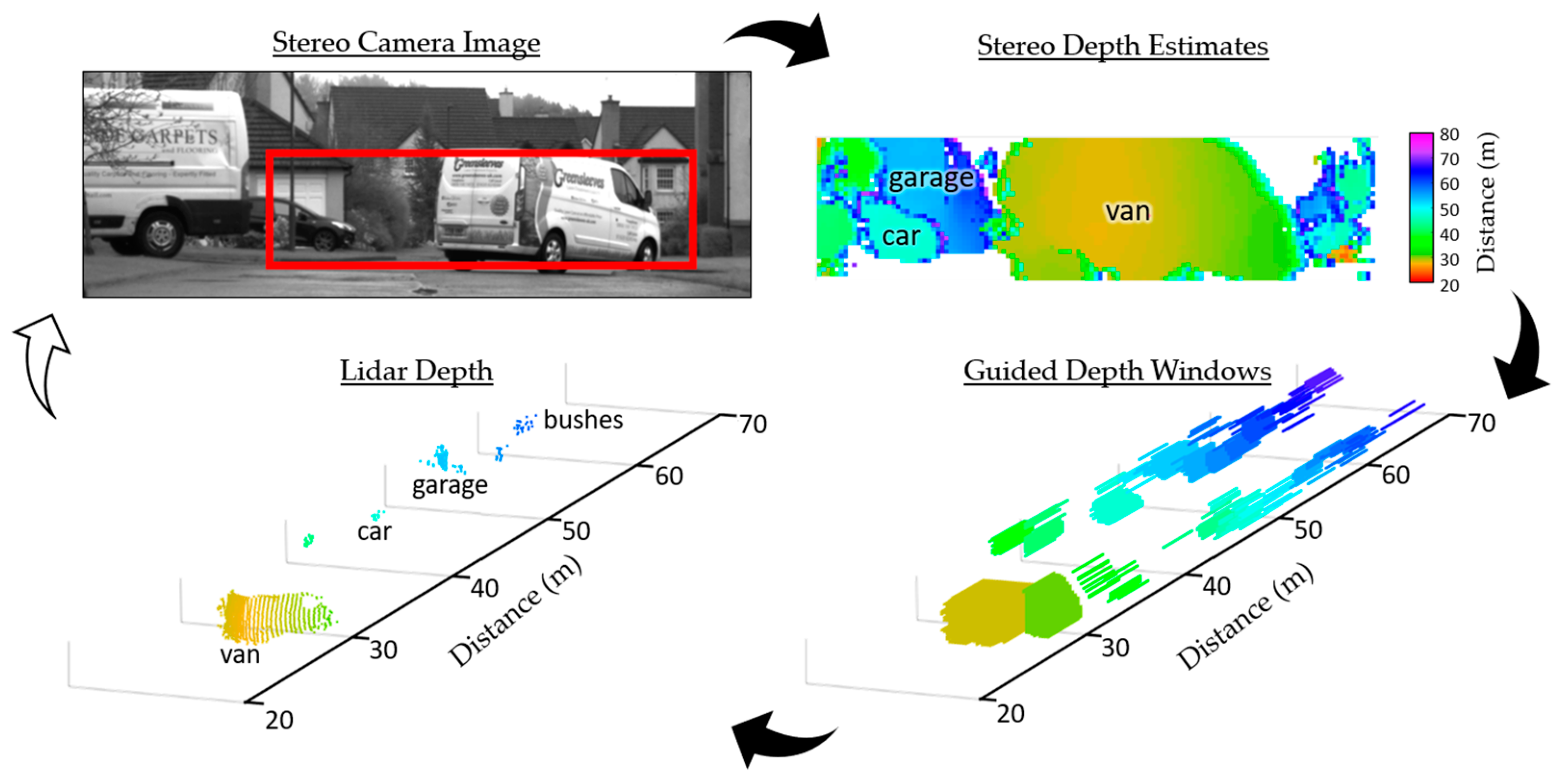
4.1. Scenes
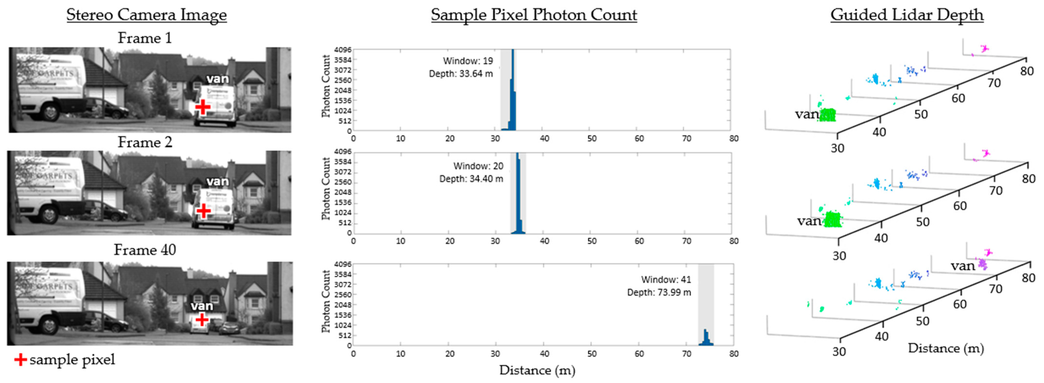
4.1.1. Outdoor Clear Conditions
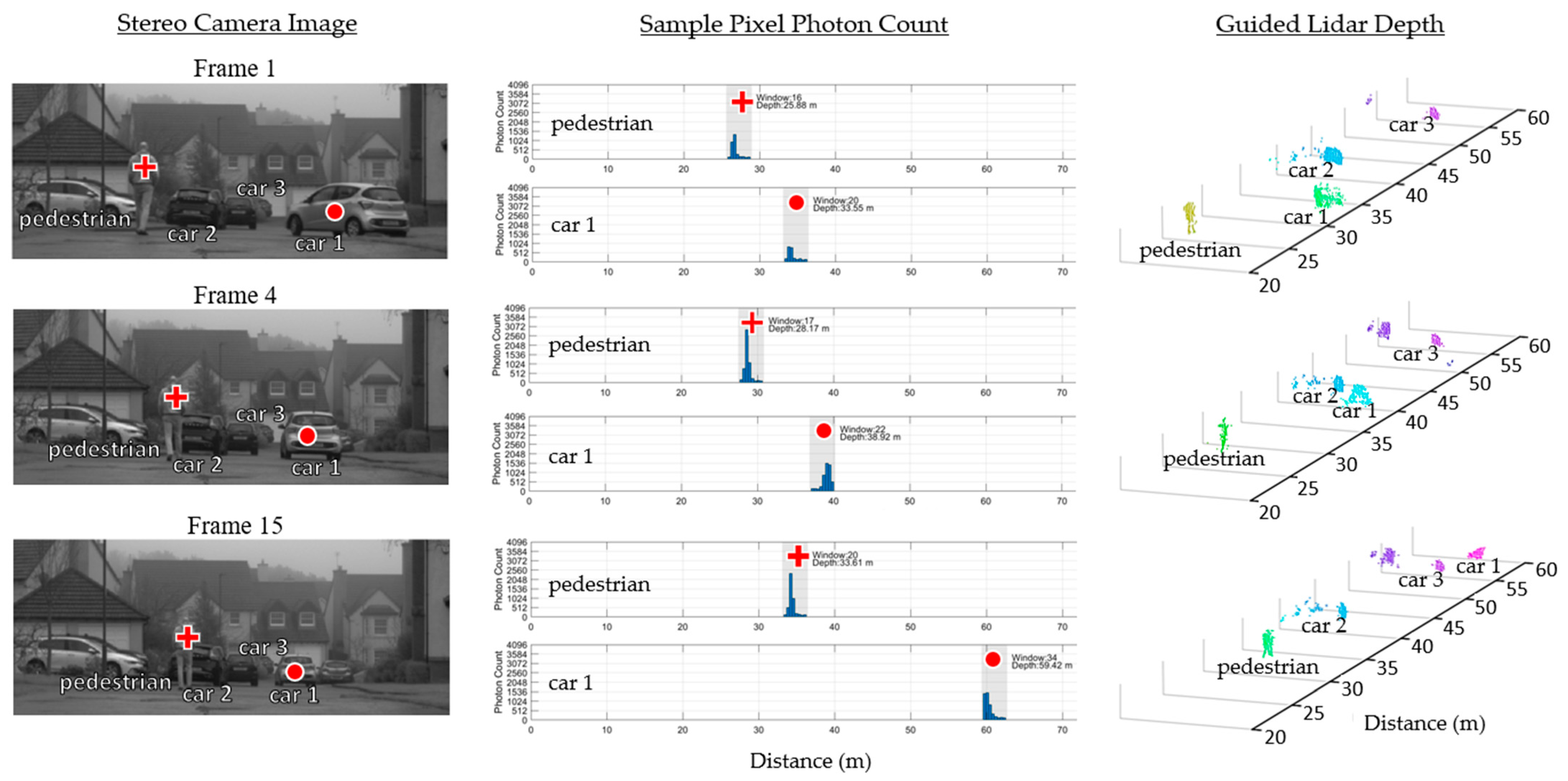
4.1.2. Outdoor Foggy Conditions
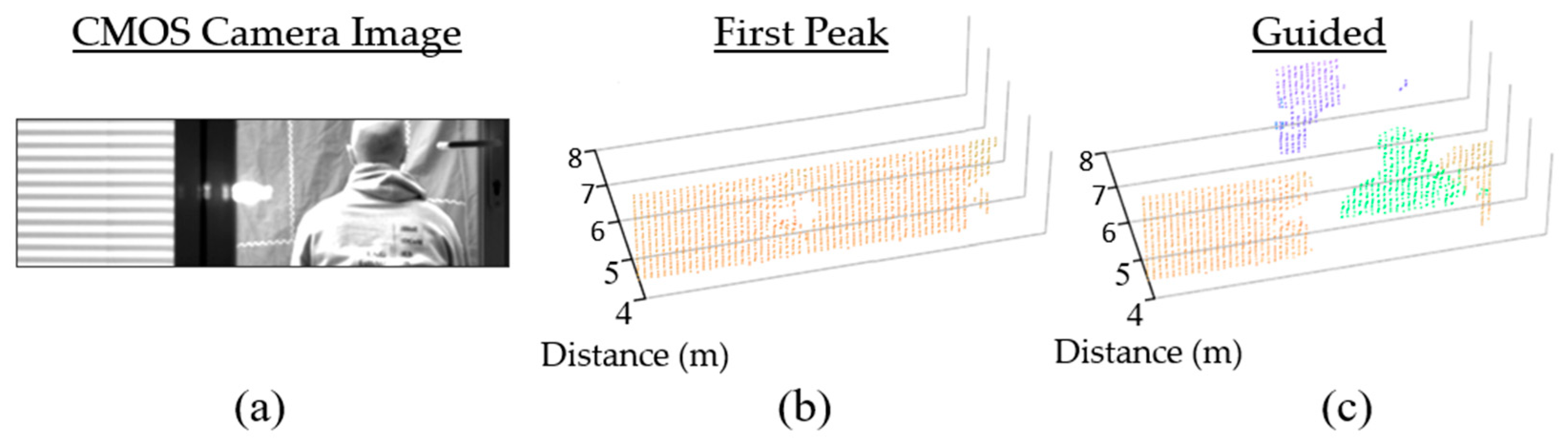
4.1.3. Transparent Obstacles
4.2. Performance
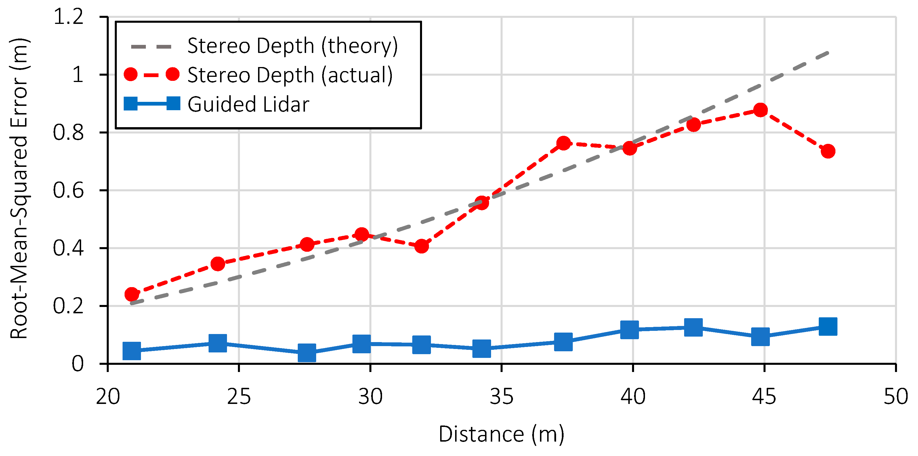
4.2.1. Measurement Error
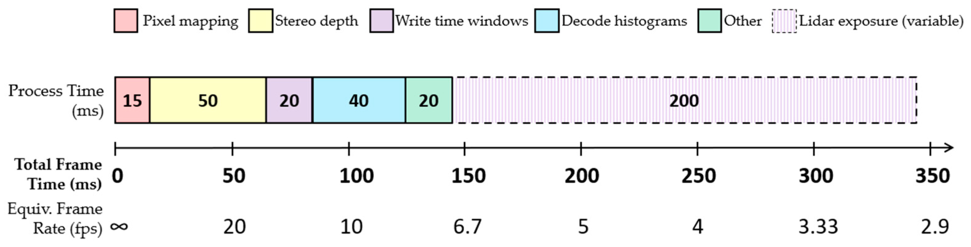
4.2.2. Processing Time
4.3. Laser Power Efficiency
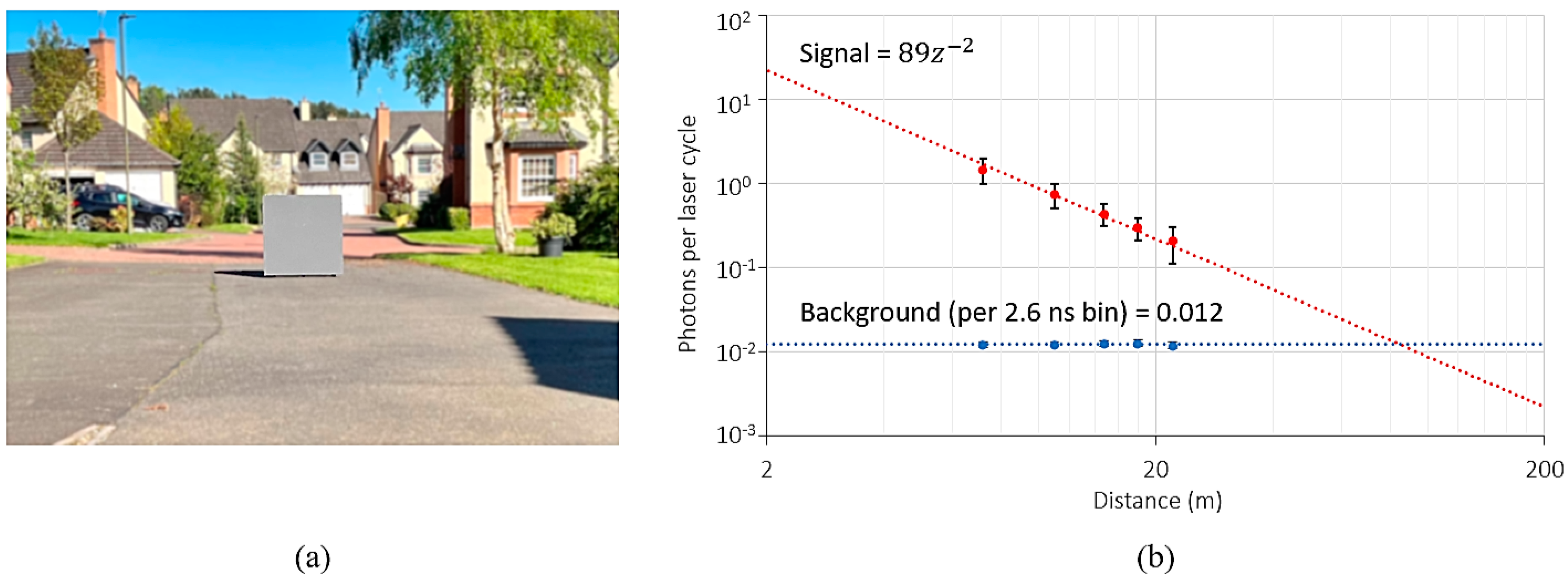
4.3.1. Lidar Characterisation
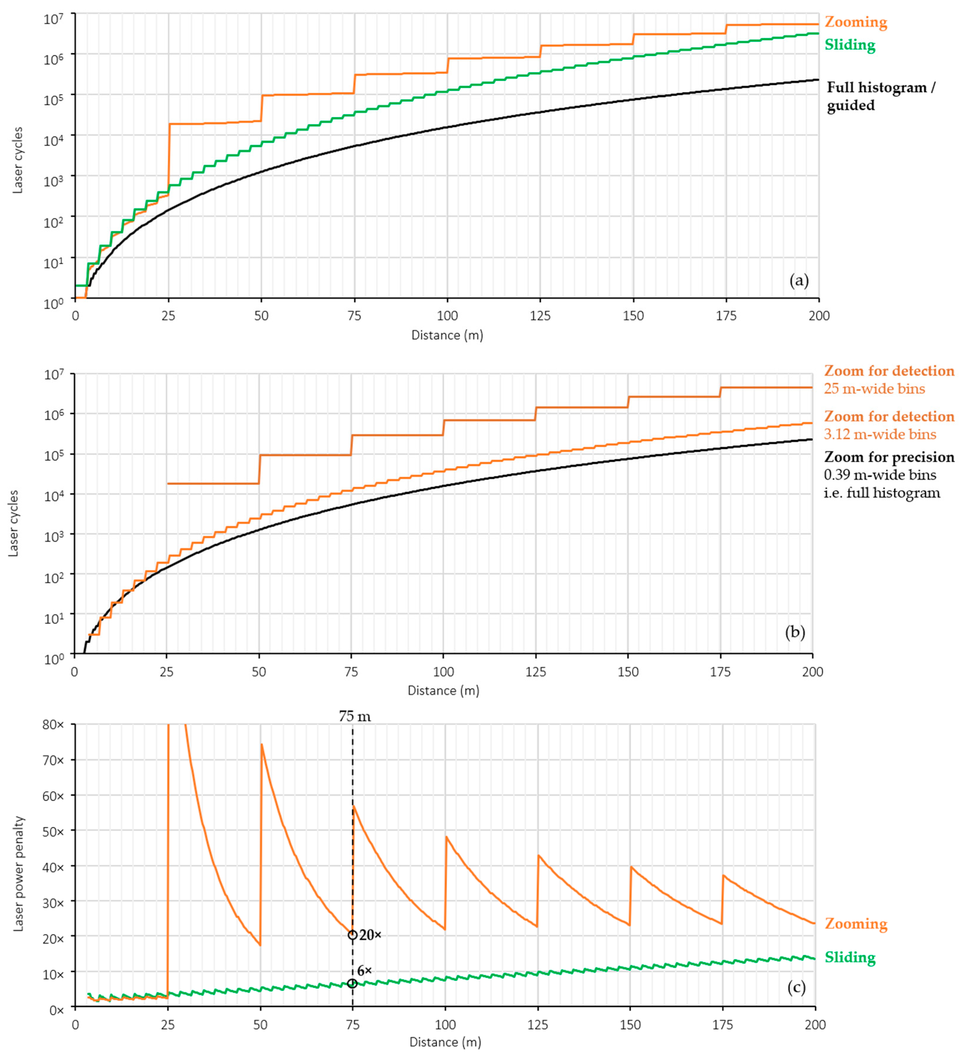
4.3.2. Laser Power Penalty of Partial Histogram Equivalent
5. Discussion
5.1. Performance Overview

| Author | Ref | Resolution (ToF pixels) | Max. Range (m) | Ambient Intensity (klux) | Precision/Accuracy (m) | Frame Rate (Hz) | Histogram Bins | Stacked | Partial Histogram |
|---|---|---|---|---|---|---|---|---|---|
| Ximenes | [17] | 64 × 128 | 300 1 | - | 0.47/0.8 | 30 2 | - | Yes | No |
| Henderson | [10] | 64 × 64 | 50 | - | -/0.17 | 30 | 16 | Yes | No |
| Zhang | [9] | 144 × 252 | 50 | - | 0.0014/0.88 | 30 2 | 8 | No | Zooming |
| Okino | [34] | 900 × 1200 | 250 | - | 1.5/- | - | - | No | No |
| Kim | [11] | 40 × 48 | 45 | - | 0.014/0.023 | - | 2 | No | Zooming |
| Kumagai | [35] | 63 × 168 | 200 | 117 | -/0.3 | 20 | - | Yes | No |
| Padmanabhan | [18] | 128 × 256 | 100 1 | 10 | -/0.07 | - | - | Yes | No |
| Stoppa | [13] | 60 × 80 | 4.4 | 50 | 0.007/0.04 | 30 | 32 | Yes | Sliding |
| Zhang | [14] | 160 × 240 | 9.5 | 10 | 0.01/0.02 | 20 | 32 | Yes | Zooming |
| Park | [15] | 60 × 80 | 45 | 30 | 0.015/0.025 | 1.5 2 | 4 | No | Zooming |
| Taloud | [16] | 32 × 42 | 8.2 | 1 | 0.007/0.03 | 30 | 59 | Yes | Sliding |
| This work | - | 32 × 64 | 75 | 70 | 0.18 | 3 | 8 | No | No |
5.2. Design Trade-Offs
5.3. Practical Challenges
5.4. Future Work
6. Conclusions
Author Contributions
Funding
Institutional Review Board Statement
Informed Consent Statement
Data Availability Statement
Acknowledgments
Conflicts of Interest
Correction Statement
Open Access
References
- Rangwala, S. Automotive LiDAR Has Arrived; Forbes: Jersey City, NJ, USA, 2022. [Google Scholar]
- Wang, Z.; Wu, Y.; Niu, Q. Multi-Sensor Fusion in Automated Driving: A Survey. IEEE Access 2020, 8, 2847–2868. [Google Scholar] [CrossRef]
- Aptiv, A.; Apollo, B.; Continenta, D.; FCA, H.; Infineon, I.V. Safety First For Automated Driving [White Paper]. Available online: https://group.mercedes-benz.com/documents/innovation/other/safety-first-for-automated-driving.pdf (accessed on 28 October 2023).
- Ford. A Matter of Trust: Ford’s Approach to Developing Self-Driving Vehicles; Ford: Detroit, MI, USA, 2018. [Google Scholar]
- Lambert, J.; Carballo, A.; Cano, A.M.; Narksri, P.; Wong, D.; Takeuchi, E.; Takeda, K. Performance Analysis of 10 Models of 3D LiDARs for Automated Driving. IEEE Access 2020, 8, 131699–131722. [Google Scholar] [CrossRef]
- Villa, F.; Severini, F.; Madonini, F.; Zappa, F. SPADs and SiPMs Arrays for Long-Range High-Speed Light Detection and Ranging (LiDAR). Sensors 2021, 21, 3839. [Google Scholar] [CrossRef] [PubMed]
- Rangwala, S. Lidar Miniaturization; ADAS & Autonomous Vehicle International: Dorking, UK, 2023; pp. 34–38. [Google Scholar]
- Niclass, C.; Soga, M.; Matsubara, H.; Ogawa, M.; Kagami, M. A 0.18 µm CMOS SoC for a 100 m-range 10 fps 200 × 96-pixel time-of-flight depth sensor. In Proceedings of the 2013 IEEE International Solid-State Circuits Conference Digest of Technical Papers, San Francisco, CA, USA, 17–21 February 2013; pp. 488–489. [Google Scholar]
- Zhang, C.; Lindner, S.; Antolović, I.M.; Pavia, J.M.; Wolf, M.; Charbon, E. A 30-frames/s, 252 × 144 SPAD Flash LiDAR with 1728 Dual-Clock 48.8-ps TDCs, and Pixel-Wise Integrated Histogramming. IEEE J. Solid State Circuits 2019, 54, 1137–1151. [Google Scholar] [CrossRef]
- Henderson, R.K.; Johnston, N.; Hutchings, S.W.; Gyongy, I.; Abbas, T.A.; Dutton, N.; Tyler, M.; Chan, S.; Leach, J. 5.7 A 256 × 256 40 nm/90 nm CMOS 3D-Stacked 120 dB Dynamic-Range Reconfigurable Time-Resolved SPAD Imager. In Proceedings of the IEEE International Solid-State Circuits Conference—(ISSCC), San Francisco, CA, USA, 17–21 February 2019; pp. 106–108. [Google Scholar]
- Kim, B.; Park, S.; Chun, J.H.; Choi, J.; Kim, S.J. 7.2 A 48 × 40 13.5 mm Depth Resolution Flash LiDAR Sensor with In-Pixel Zoom Histogramming Time-to-Digital Converter. In Proceedings of the 2021 IEEE International Solid- State Circuits Conference (ISSCC), San Francisco, CA, USA, 13–22 February 2021; pp. 108–110. [Google Scholar]
- Gyongy, I.; Erdogan, A.T.; Dutton, N.A.; Mai, H.; Rocca, F.M.D.; Henderson, R.K. A 200kFPS, 256 × 128 SPAD dToF sensor with peak tracking and smart readout. In Proceedings of the International Image Sensor Workshop, Virtual, 20–23 September 2021. [Google Scholar]
- Stoppa, D.; Abovyan, S.; Furrer, D.; Gancarz, R.; Jessenig, T.; Kappel, R.; Lueger, M.; Mautner, C.; Mills, I.; Perenzoni, D.; et al. A Reconfigurable QVGA/Q3VGA Direct Time-of-Flight 3D Imaging System with On-chip Depth-map Computation in 45/40 nm 3D-stacked BSI SPAD CMOS. In Proceedings of the International Image Sensor Workshop, Virtual, 20–23 September 2021. [Google Scholar]
- Zhang, C.; Zhang, N.; Ma, Z.; Wang, L.; Qin, Y.; Jia, J.; Zang, K. A 240 × 160 3D Stacked SPAD dToF Image Sensor with Rolling Shutter and In Pixel Histogram for Mobile Devices. IEEE Open J. Solid State Circuits Soc. 2021, 2, 3–11. [Google Scholar] [CrossRef]
- Park, S.; Kim, B.; Cho, J.; Chun, J.; Choi, J.; Kim, S. 5.3 An 80 × 60 Flash LiDAR Sensor with In-Pixel Histogramming TDC Based on Quaternary Search and Time-Gated Δ-Intensity Phase Detection for 45m Detectable Range and Background Light Cancellation. In Proceedings of the 2022 IEEE International Solid-State Circuits Conference (ISSCC), San Francisco, CA, USA, 20–26 February 2022. [Google Scholar]
- Taloud, P.-Y.; Bernhard, S.; Biber, A.; Boehm, M.; Chelvam, P.; Cruz, A.; Chele, A.D.; Gancarz, R.; Ishizaki, K.; Jantscher, P.; et al. A 1.2 K dots dToF 3D Imaging System in 45/22 nm 3D-stacked BSI SPAD CMOS. In Proceedings of the International SPAD Sensor Workshop, Virtual, 13–15 June 2022. [Google Scholar]
- Ximenes, A.R.; Padmanabhan, P.; Lee, M.J.; Yamashita, Y.; Yaung, D.N.; Charbon, E. A 256 × 256 45/65 nm 3D-stacked SPAD-based direct TOF image sensor for LiDAR applications with optical polar modulation for up to 18.6dB interference suppression. In Proceedings of the 2018 IEEE International Solid-State Circuits Conference—(ISSCC), San Francisco, CA, USA, 11–15 February 2018; pp. 96–98. [Google Scholar]
- Padmanabhan, P.; Zhang, C.; Cazzaniga, M.; Efe, B.; Ximenes, A.R.; Lee, M.J.; Charbon, E. 7.4 A 256 × 128 3D-Stacked (45 nm) SPAD FLASH LiDAR with 7-Level Coincidence Detection and Progressive Gating for 100 m Range and 10 klux Background Light. In Proceedings of the 2021 IEEE International Solid-State Circuits Conference (ISSCC), San Francisco, CA, USA, 13–22 February 2021; pp. 111–113. [Google Scholar]
- Taneski, F.; Gyongy, I.; Abbas, T.A.; Henderson, R. Guided Flash Lidar: A Laser Power Efficient Approach for Long-Range Lidar. In Proceedings of the International Image Sensor Workshop, Crieff, UK, 21–25 May 2023. [Google Scholar]
- Sudhakar, S.; Sze, V.; Karaman, S. Data Centers on Wheels: Emissions from Computing Onboard Autonomous Vehicles. IEEE Micro 2023, 43, 29–39. [Google Scholar] [CrossRef]
- Taneski, F.; Abbas, T.A.; Henderson, R.K. Laser Power Efficiency of Partial Histogram Direct Time-of-Flight LiDAR Sensors. J. Light. Technol. 2022, 40, 5884–5893. [Google Scholar] [CrossRef]
- Fisher, R.B. Subpixel Estimation. In Computer Vision; Springer: Berlin/Heidelberg, Germany, 2021; pp. 1217–1220. [Google Scholar]
- Geiger, A.; Lenz, P.; Urtasun, R. Are we ready for autonomous driving? The KITTI vision benchmark suite. In Proceedings of the 2012 IEEE Conference on Computer Vision and Pattern Recognition, Providence, RI, USA, 16–21 June 2012; pp. 3354–3361. [Google Scholar]
- Laga, H.; Jospin, L.V.; Boussaid, F.; Bennamoun, M. A Survey on Deep Learning Techniques for Stereo-Based Depth Estimation. IEEE Trans. Pattern Anal. Mach. Intell. 2022, 44, 1738–1764. [Google Scholar] [CrossRef] [PubMed]
- Hirschmuller, H. Stereo Processing by Semiglobal Matching and Mutual Information. IEEE Trans. Pattern Anal. Mach. Intell. 2008, 30, 328–341. [Google Scholar] [CrossRef] [PubMed]
- Zhang, Z. A flexible new technique for camera calibration. IEEE Trans. Pattern Anal. Mach. Intell. 2000, 22, 1330–1334. [Google Scholar] [CrossRef]
- MATLAB; R2023b; MathWorks: Natick, MA, USA, 2023.
- Koerner, L.J. Models of Direct Time-of-Flight Sensor Precision That Enable Optimal Design and Dynamic Configuration. IEEE Trans. Instrum. Meas. 2021, 70, 1–9. [Google Scholar] [CrossRef]
- Bijelic, M.; Gruber, T.; Ritter, W. A Benchmark for Lidar Sensors in Fog: Is Detection Breaking Down? In Proceedings of the 2018 IEEE Intelligent Vehicles Symposium (IV), Suzhou, China, 26–30 June 2018; pp. 760–767. [Google Scholar]
- Gyongy, I.; Dutton, N.A.; Henderson, R.K. Direct Time-of-Flight Single-Photon Imaging. IEEE Trans. Electron Devices 2022, 69, 2794–2805. [Google Scholar] [CrossRef]
- Tontini, A.; Gasparini, L.; Perenzoni, M. Numerical Model of SPAD-Based Direct Time-of-Flight Flash LIDAR CMOS Image Sensors. Sensor 2020, 20, 5203. [Google Scholar] [CrossRef] [PubMed]
- Wallace, A.M.; Halimi, A.; Buller, G.S. Full Waveform LiDAR for Adverse Weather Conditions. IEEE Trans. Veh. Technol. 2020, 69, 7064–7077. [Google Scholar] [CrossRef]
- Schönlieb, A.; Lugitsch, D.; Steger, C.; Holweg, G.; Druml, N. Multi-Depth Sensing for Applications With Indirect Solid-State LiDAR. In Proceedings of the 2020 IEEE Intelligent Vehicles Symposium (IV), Las Vegas, NV, USA, 19 October–13 November 2020; pp. 919–925. [Google Scholar]
- Okino, T.; Yamada, S.; Sakata, Y.; Kasuga, S.; Takemoto, M.; Nose, Y.; Koshida, H.; Tamaru, M.; Sugiura, Y.; Saito, S.; et al. 5.2 A 1200 × 900 6 µm 450 fps Geiger-Mode Vertical Avalanche Photodiodes CMOS Image Sensor for a 250m Time-of-Flight Ranging System Using Direct-Indirect-Mixed Frame Synthesis with Configurable-Depth-Resolution Down to 10cm. In Proceedings of the 2020 IEEE International Solid-State Circuits Conference (ISSCC), San Francisco, CA, USA, 16–20 February 2020; pp. 96–98. [Google Scholar]
- Kumagai, O.; Ohmachi, J.; Matsumura, M.; Yagi, S.; Tayu, K.; Amagawa, K.; Matsukawa, T.; Ozawa, O.; Hirono, D.; Shinozuka, Y.; et al. 7.3 A 189 × 600 Back-Illuminated Stacked SPAD Direct Time-of-Flight Depth Sensor for Automotive LiDAR Systems. In Proceedings of the 2021 IEEE International Solid- State Circuits Conference (ISSCC), San Francisco, CA, USA, 13–22 February 2021; pp. 110–112. [Google Scholar]
- Badki, A.; Troccoli, A.; Kim, K.; Kautz, J.; Sen, P.; Gallo, O. Bi3D: Stereo Depth Estimation via Binary Classifications. In Proceedings of the IEEE/CVF Conference on Computer Vision and Pattern Recognition, Seattle, WA, USA, 14–19 June 2020. [Google Scholar]
- Dang, T.; Hoffmann, C.; Stiller, C. Continuous Stereo Self-Calibration by Camera Parameter Tracking. IEEE Trans. Image Process. 2009, 18, 1536–1550. [Google Scholar] [CrossRef]
- Warren, M.E. Automotive LIDAR Technology. In Proceedings of the 2019 Symposium on VLSI Circuits, Kyoto, Japan, 9–14 June 2019; pp. C254–C255. [Google Scholar]
- Morimoto, K.; Iwata, J.; Shinohara, M.; Sekine, H.; Abdelghafar, A.; Tsuchiya, H.; Kuroda, Y.; Tojima, K.; Endo, W.; Maehashi, Y.; et al. 3.2 Megapixel 3D-Stacked Charge Focusing SPAD for Low-Light Imaging and Depth Sensing. In Proceedings of the 2021 IEEE International Electron Devices Meeting (IEDM), San Francisco, CA, USA, 11–16 December 2021; pp. 20.2.1–20.2.4. [Google Scholar]


| Parameter | Full Histogram | Partial Histogram | Guided | |
|---|---|---|---|---|
| Zooming | Sliding | |||
| Laser power penalty | Low | High | High | Low |
| Area requirement | High | Low | Low | Low |
| Data volume | High | Low | High | Low |
| Multipath reflection artefacts | Low | Medium | Low | Low |
| Motion artefacts | Low | Medium | Medium | Medium |
| System complexity | Low | Low | Low | High |
| Component | Parameter | Value |
|---|---|---|
| Stereo Rig | Baseline | 1 m |
| Camera model | FLIR BFS-U3-16S2M-CS | |
| Maximum resolution | 1080 × 1440 | |
| Focal length | 12 mm | |
| Lidar | Laser pulse width | 4.5 ns FWHM |
| Laser repetition rate | 80 kHz | |
| Wavelength | 940 nm | |
| Filter bandwidth | 10 nm FWHM | |
| Focal length | 25 mm | |
| Field of view (H × V) | 16° × 4° | |
| Histogram bins | 8 × 12-bit | |
| Histogram bin width | 0.39 m (2.6 ns) | |
| Histogram window step | 1.875 m (1.25 ns) |
Disclaimer/Publisher’s Note: The statements, opinions and data contained in all publications are solely those of the individual author(s) and contributor(s) and not of MDPI and/or the editor(s). MDPI and/or the editor(s) disclaim responsibility for any injury to people or property resulting from any ideas, methods, instructions or products referred to in the content. |
© 2023 by the authors. Licensee MDPI, Basel, Switzerland. This article is an open access article distributed under the terms and conditions of the Creative Commons Attribution (CC BY) license (https://creativecommons.org/licenses/by/4.0/).
Share and Cite
Taneski, F.; Gyongy, I.; Al Abbas, T.; Henderson, R.K. Guided Direct Time-of-Flight Lidar Using Stereo Cameras for Enhanced Laser Power Efficiency. Sensors 2023, 23, 8943. https://doi.org/10.3390/s23218943
Taneski F, Gyongy I, Al Abbas T, Henderson RK. Guided Direct Time-of-Flight Lidar Using Stereo Cameras for Enhanced Laser Power Efficiency. Sensors. 2023; 23(21):8943. https://doi.org/10.3390/s23218943
Chicago/Turabian StyleTaneski, Filip, Istvan Gyongy, Tarek Al Abbas, and Robert K. Henderson. 2023. "Guided Direct Time-of-Flight Lidar Using Stereo Cameras for Enhanced Laser Power Efficiency" Sensors 23, no. 21: 8943. https://doi.org/10.3390/s23218943
APA StyleTaneski, F., Gyongy, I., Al Abbas, T., & Henderson, R. K. (2023). Guided Direct Time-of-Flight Lidar Using Stereo Cameras for Enhanced Laser Power Efficiency. Sensors, 23(21), 8943. https://doi.org/10.3390/s23218943