
Intelligent Fault Diagnosis of Rolling Bearings Based on a Complete Frequency Range Feature Extraction and Combined Feature Selection Methodology

Abstract
:1. Introduction
2. Methods
2.1. BCMFDE
2.1.1. FDE
- The time series is mapped to through the Normal Cumulative Distribution Function (NCDF). Each element in vector is defined as:
- 2.
- Each element is mapped to a new symbolic sequence using a linear transformation as follows:
- 3.
- The series with the embedding dimension and the delay time are constructed as follows:
- 4.
- The fuzzy membership function is introduced in sequence as follows:
- 5.
- Each vector is mapped to a dispersion pattern according to its degrees of membership. where is class , is class ,, and is class . The membership degree of each vector is calculated to obtain the membership degree of each dispersion pattern:
- 6.
- The probability of each dispersion pattern is calculated as follows:
- 7.
- Finally, the FDE is calculated according to the theory of Shannon’s entropy as follows:
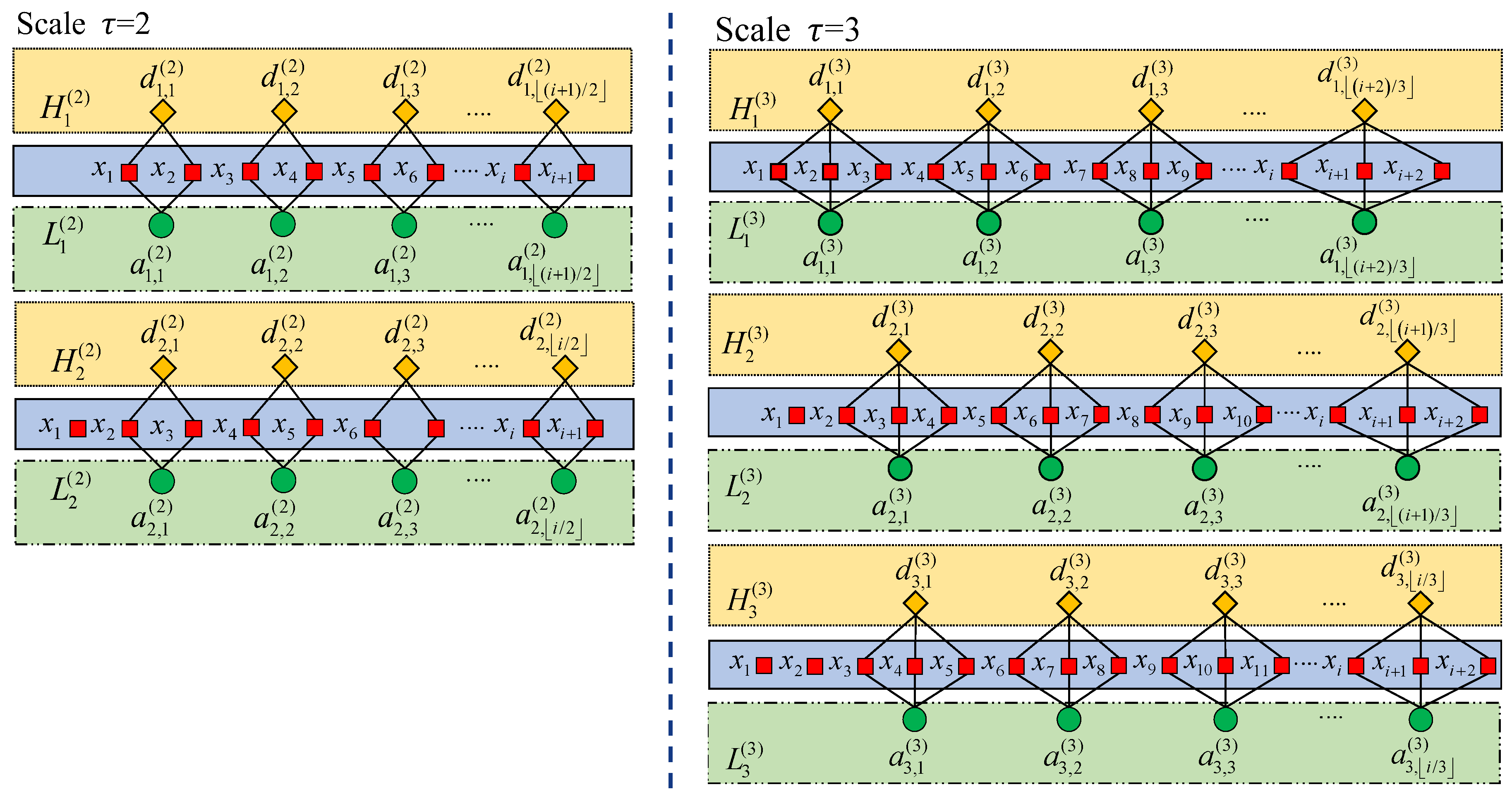
2.1.2. BCCGP
- 1.
- For time series of length, is a positive integer, and the bidirectional composite coarse-graining operator at scales factors is expressed as
- 2.
- The coarse-grained series form of operators and is expressed as:
- 3.
- According to the definition of FDE, the BCMFDE is obtained by
2.2. Feature Selection
2.2.1. RF
- 1.
- The corresponding OOB data are selected for each decision tree to calculate the OOB data error rate, denoted as .
- 2.
- The OOB data error rate is calculated again after adding random noise interference to all samples of OOB data and is denoted as .
- 3.
- The importance of the feature when there are decision trees in the forest can be expressed as:
2.2.2. mRMR
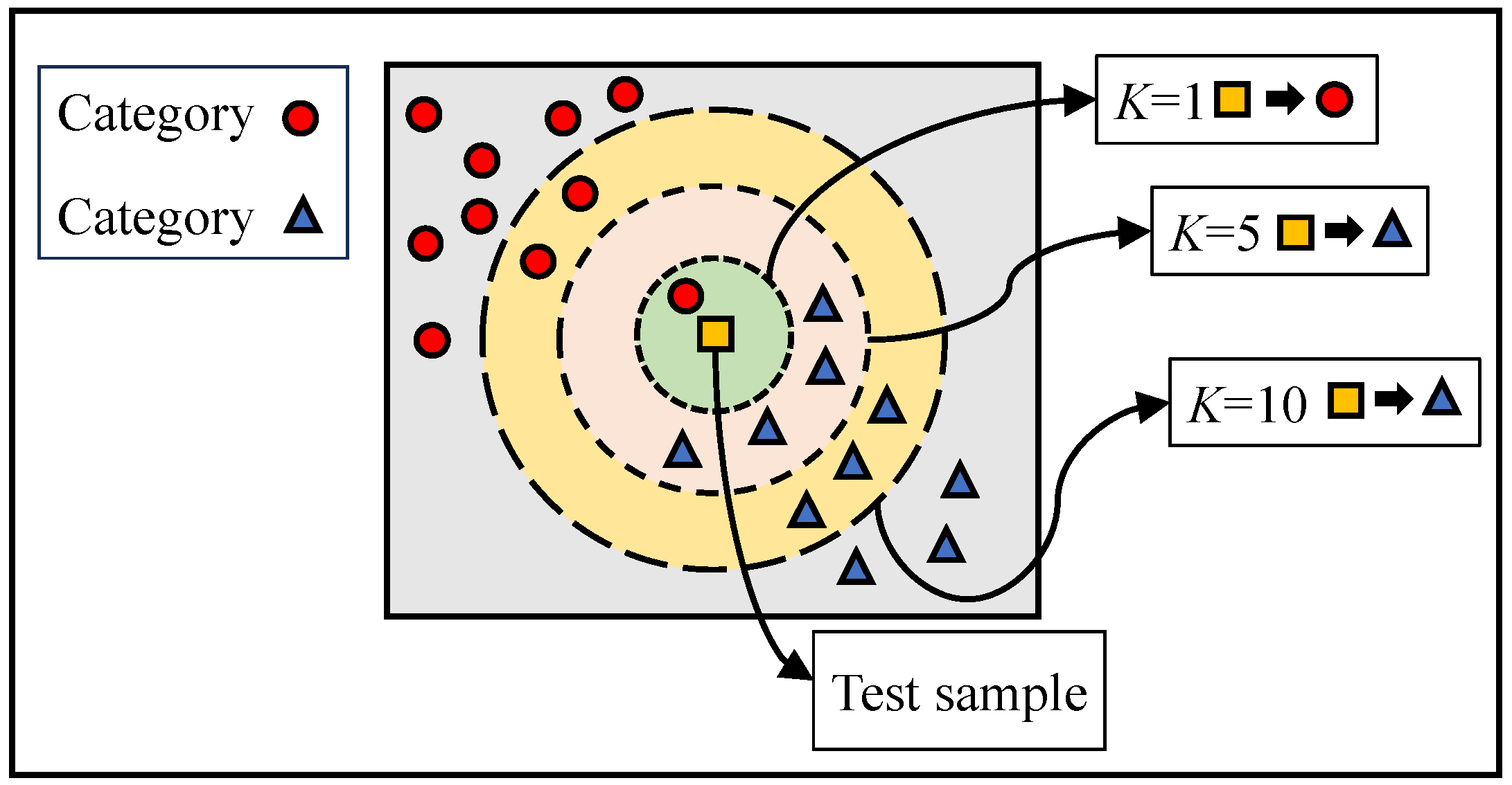
2.3. KNN
- Calculating the distance between the feature data of the test sample and the feature data of each training sample.
- Ranking the distance according to its magnitude.
- Selecting the samples with the smallest distance.
- Calculating the frequency of occurrence of the category in which the top samples are located.
- Returning the category with the highest occurrence frequency among the top samples as the classification of the test sample.
3. Intelligent Fault Diagnosis Framework
- Step 1: Signal acquisition as shown in Figure 3a. The vibration sensor is used to collect the dynamic response for bearing condition diagnosis. The collected vibration signal is segmented with equal length before the signal being analyzed.
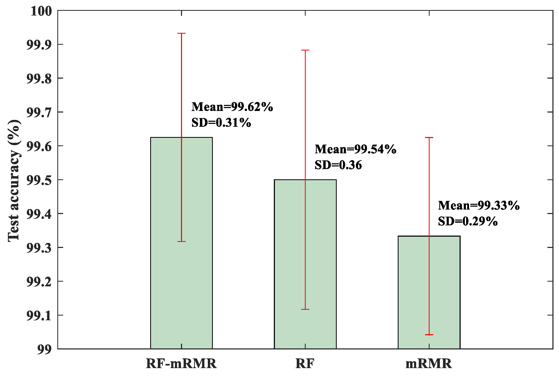
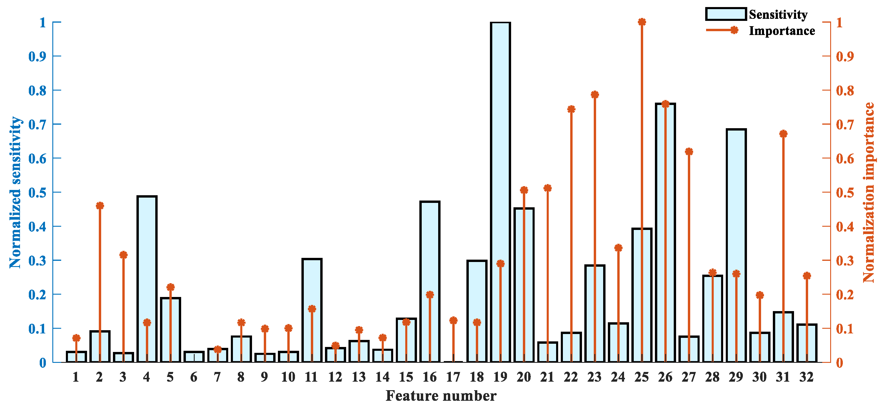
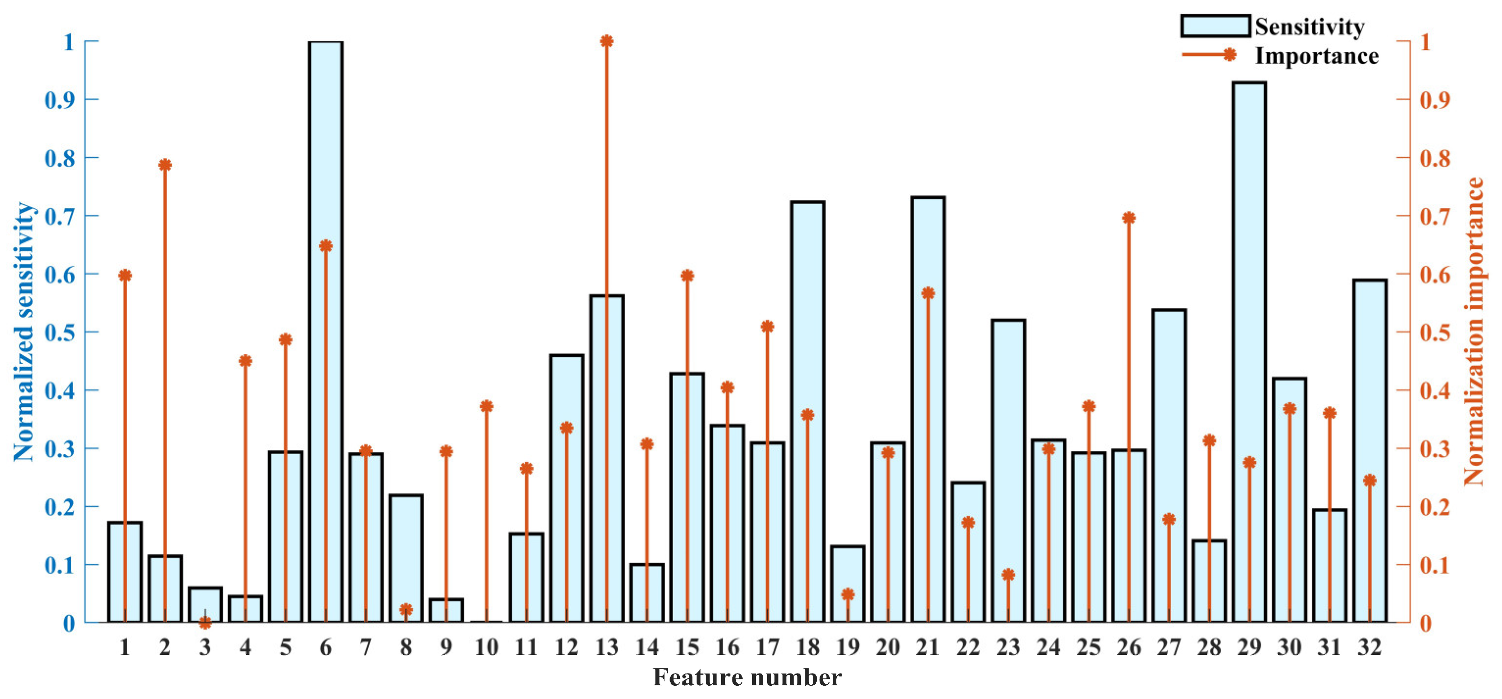
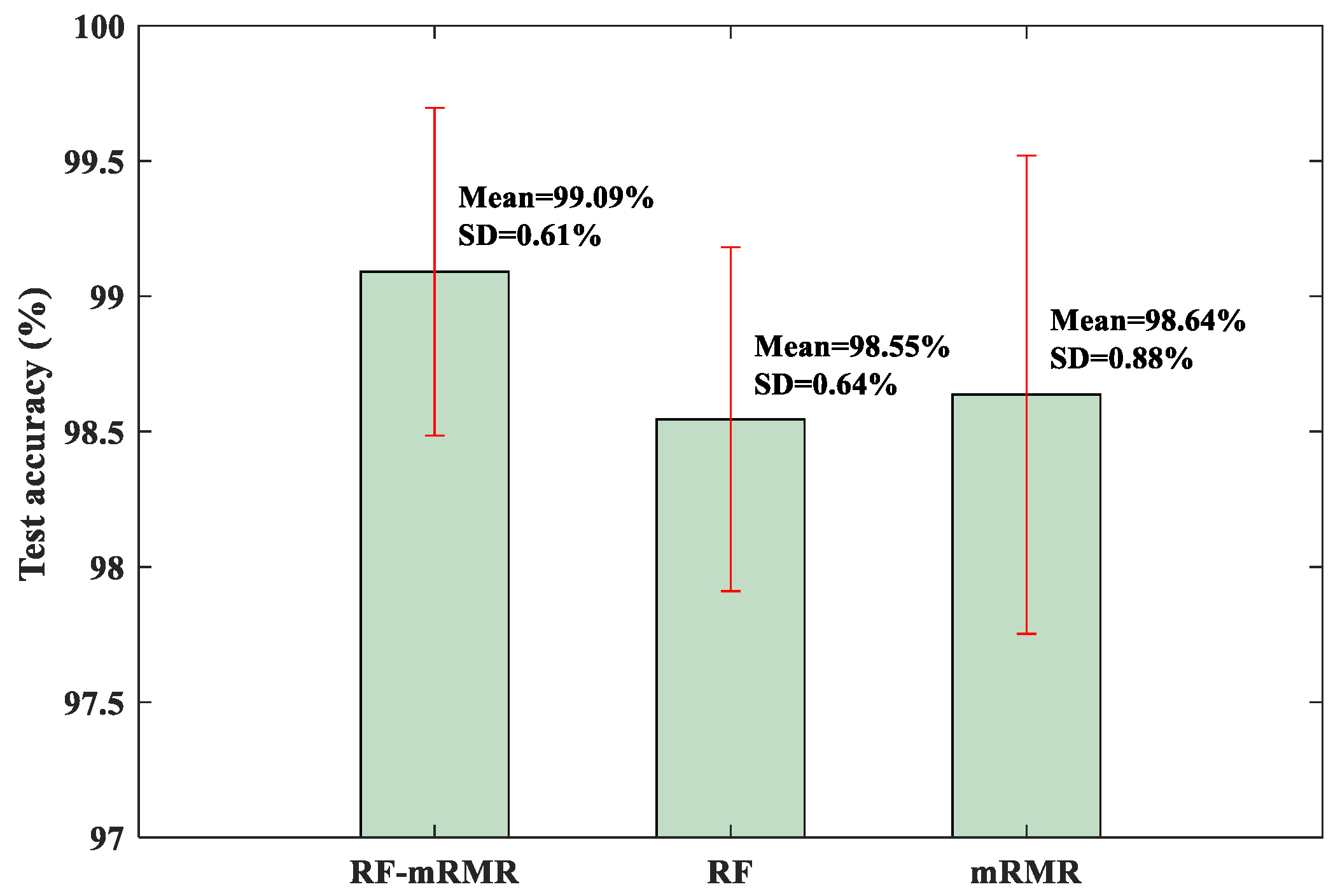
- Step 2: Feature sets construction as shown in Figure 3b. Firstly, the analyzed signal is subjected to BCCGP processing to obtain the low-frequency and high-frequency component series in different scales. The FDE of each series is calculated using Equation (12). The alternative feature set of rolling bearing faults consisting of BCMFDE is constructed. Secondly, the RF-mRMR is used to select the dominant features from the rolling bearing alternative feature set based on the importance and sensitivity of features at each scale to obtain a new rolling bearing fault feature set.
- Step 3: Failure identification and classification as shown in Figure 3c. The new rolling bearing fault feature set is randomly divided into a training sample set and a test sample set. The training sample set is used to train the KNN classifier. The test samples are used as input to the trained KNN classifier to test the classifier’s ability to identify rolling bearing health conditions in rotating machinery.

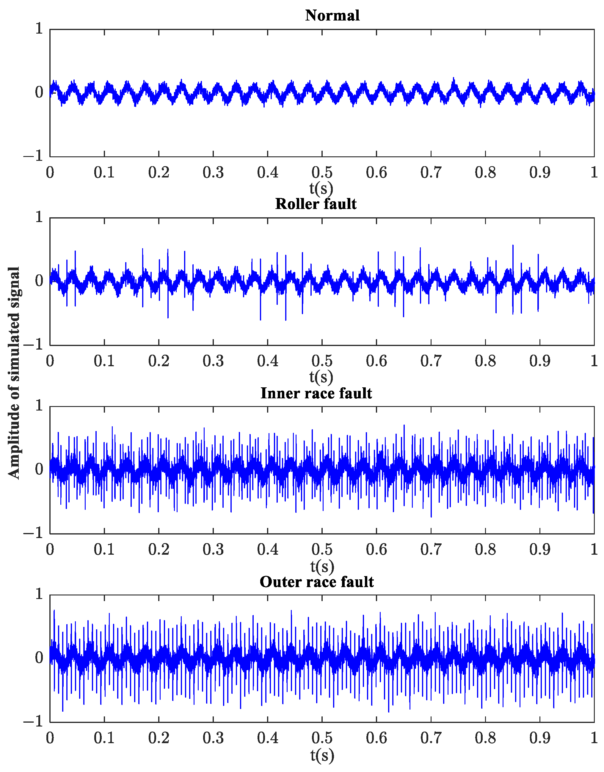
4. Simulation
4.1. Simulated Bearing Damage Vibration Response
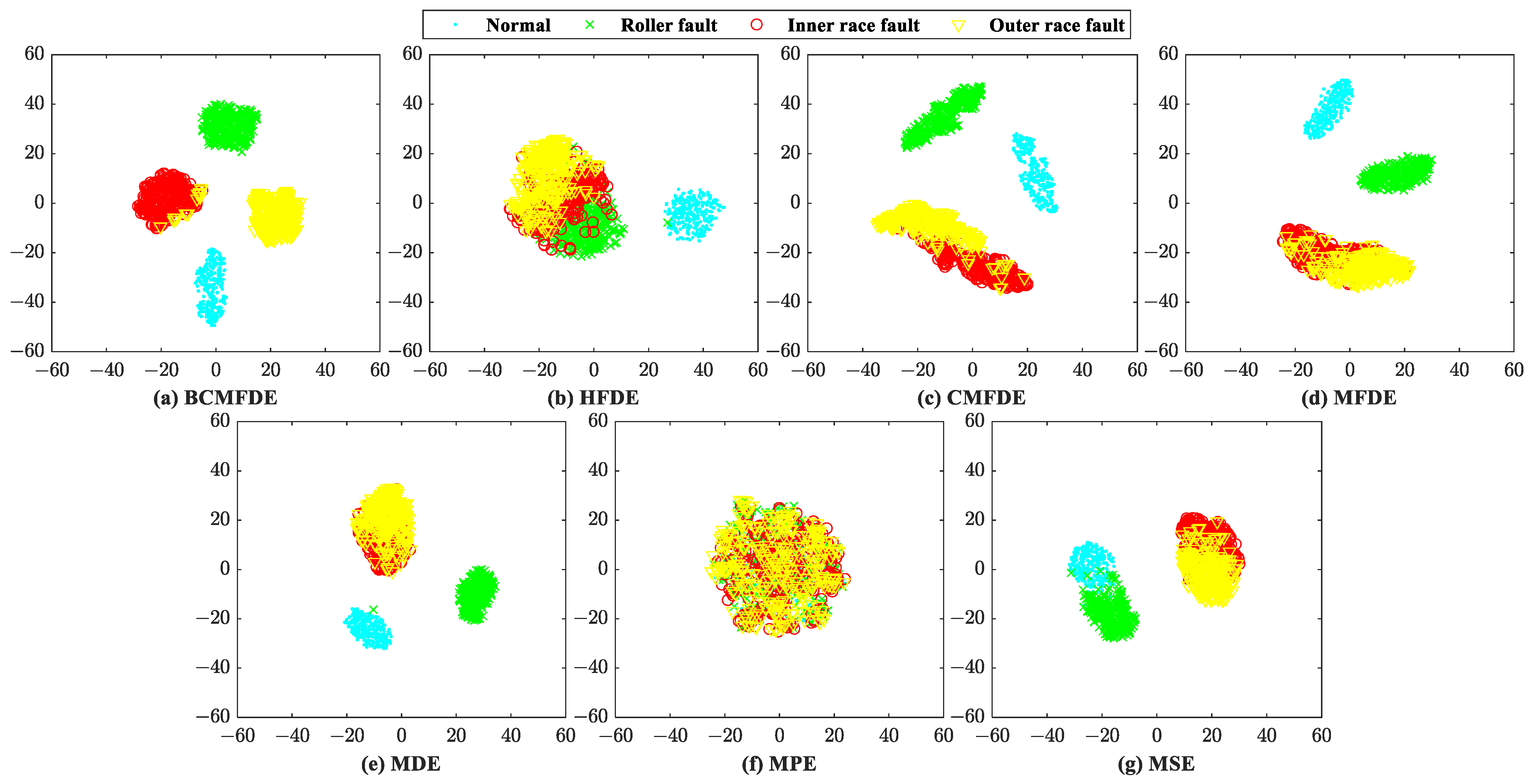
4.2. Simulation Analysis
5. Experimental Validation
5.1. Example 1: Rolling Bearing Fault Category Identification
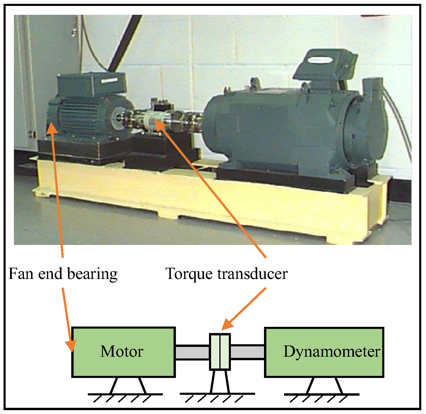
5.1.1. Test Setup
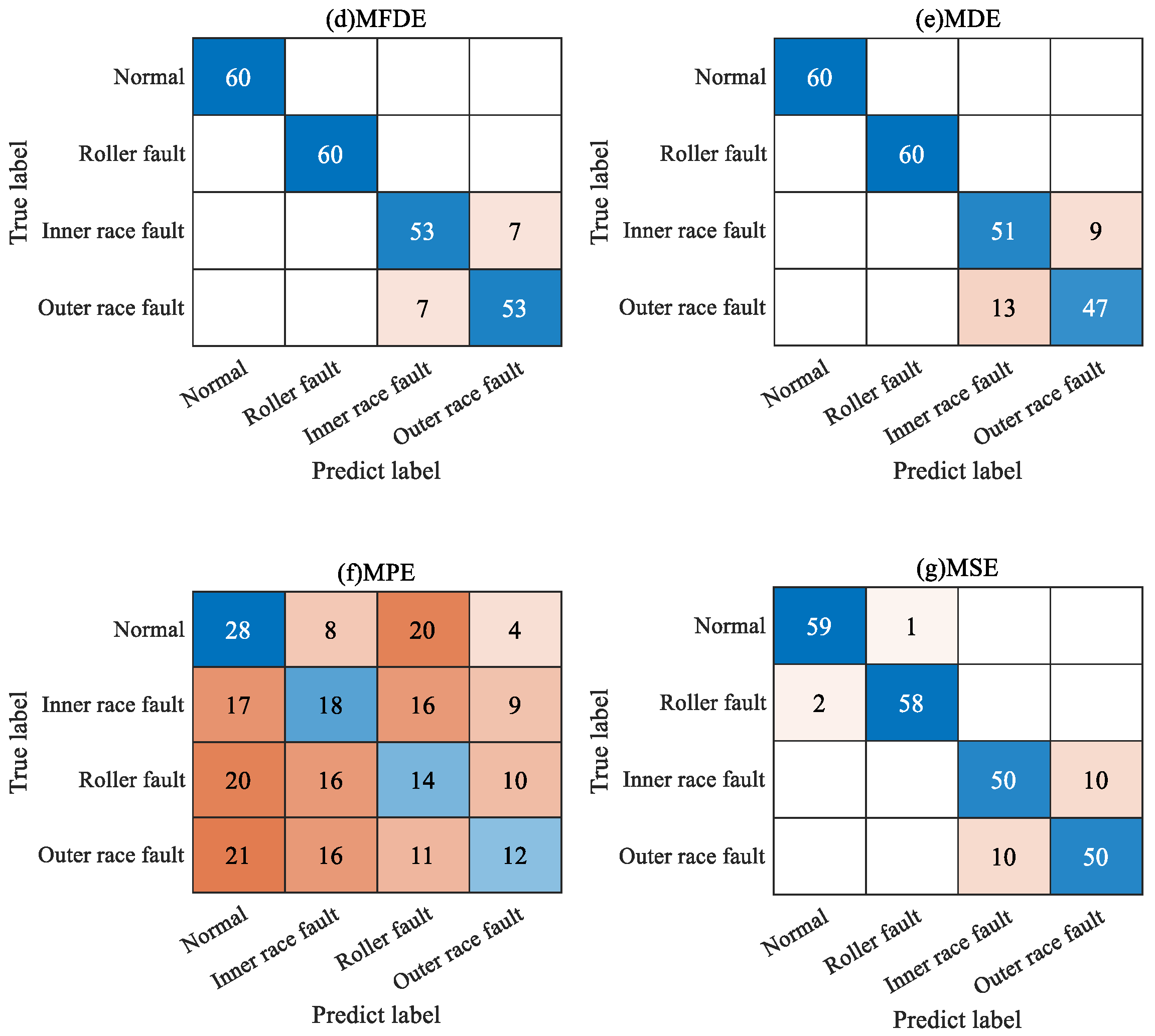
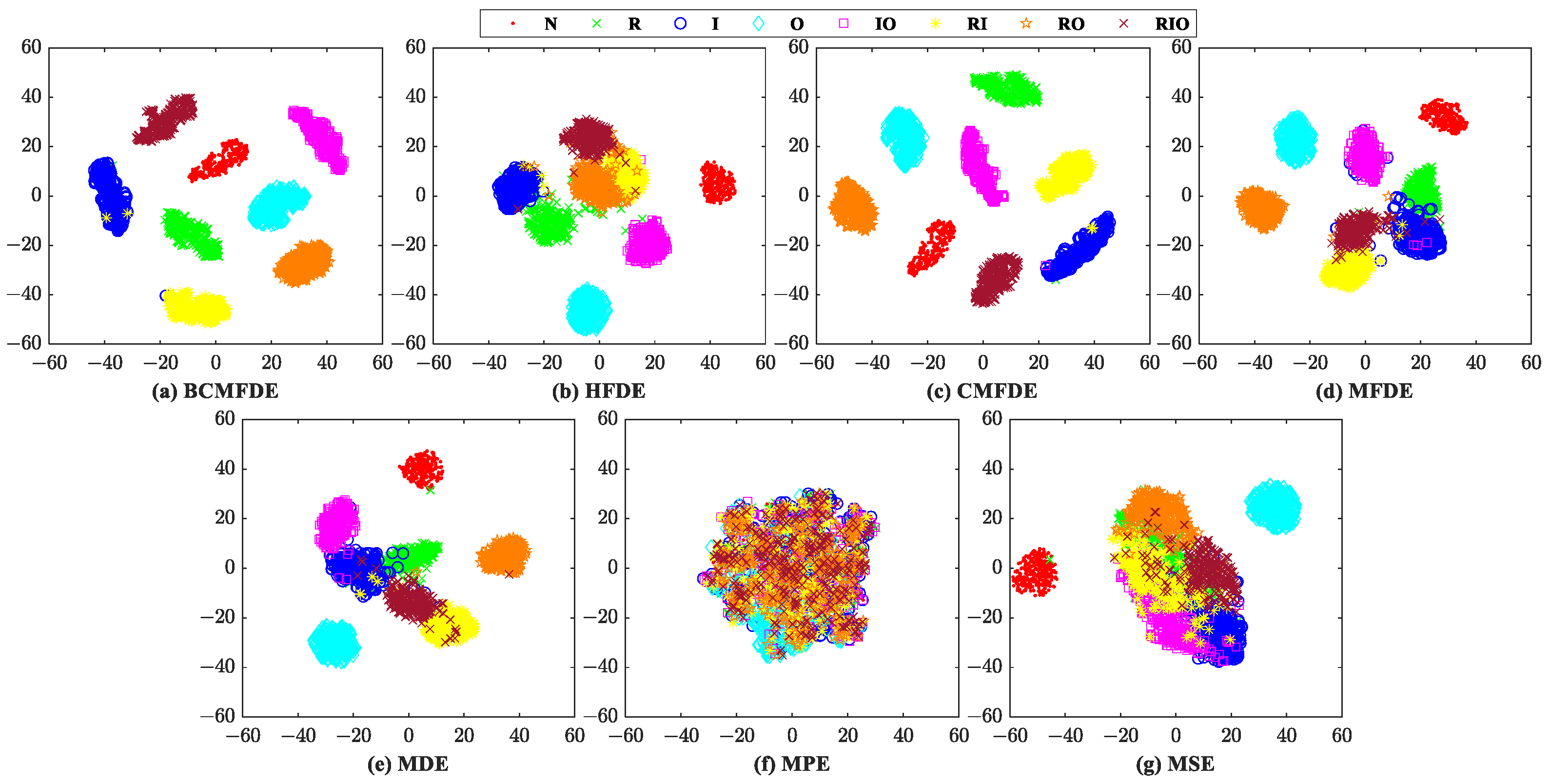
5.1.2. Diagnosis Results and Analysis
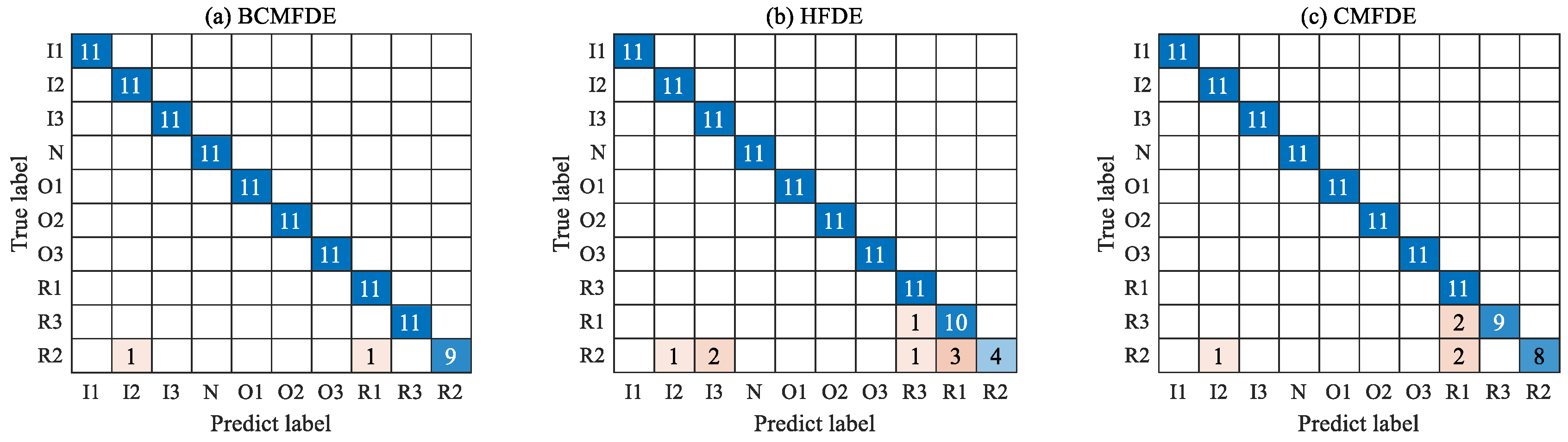
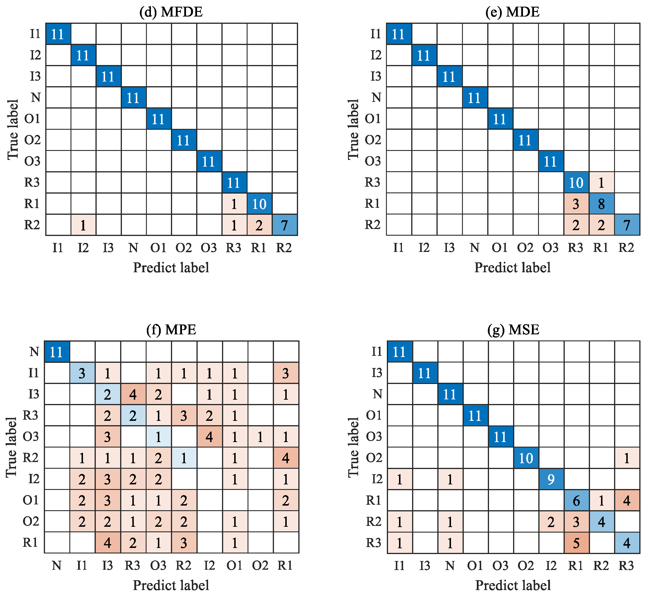
5.2. Example 2: Rolling Bearing Fault Category and Severity Identification
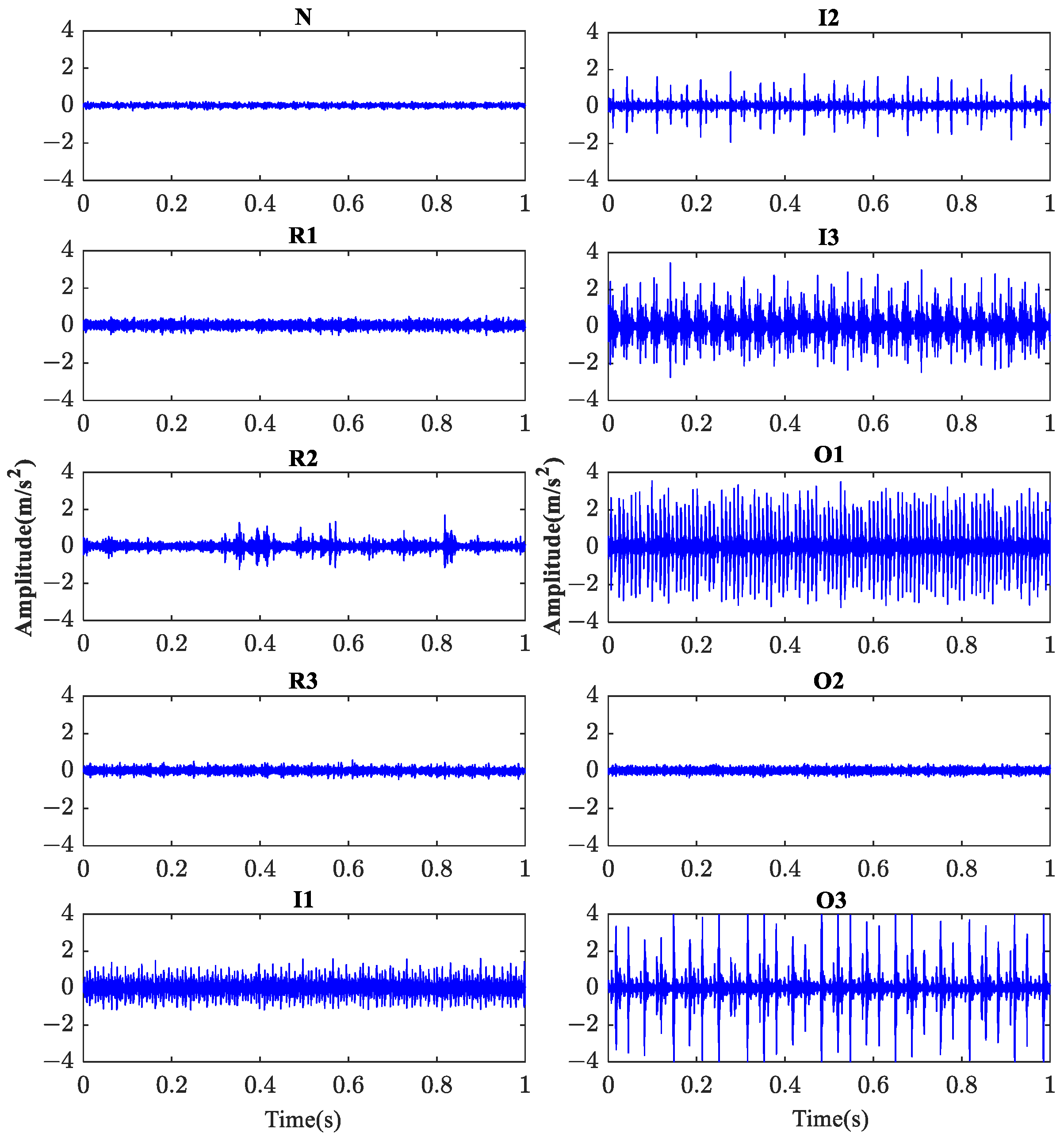
5.2.1. The Test Data
5.2.2. Diagnosis Results and Analysis
6. Conclusions
Author Contributions
Funding
Institutional Review Board Statement
Informed Consent Statement
Data Availability Statement
Conflicts of Interest
References
- Jardine, A.K.S.; Lin, D.; Banjevic, D. A review on machinery diagnostics and prognostics implementing condition-based maintenance. Mech. Syst. Signal. Process. 2006, 20, 1483–1510. [Google Scholar] [CrossRef]
- Zhang, X.; Miao, Q.; Zhang, H.; Wang, L. A parameter-adaptive VMD method based on grasshopper optimization algorithm to analyze vibration signals from rotating machinery. Mech. Syst. Signal. Process. 2018, 108, 58–72. [Google Scholar] [CrossRef]
- Cerrada, M.; Sanchez, R.V.; Li, C.; Pacheco, F.; Cabrera, D.; Oliveira, J.V.; Vsquez, R.E. A review on data-driven fault severity assessment in rolling bearings. Mech. Syst. Signal. Process. 2018, 99, 169–196. [Google Scholar] [CrossRef]
- Wang, D.; Tsui, K.L. Statistical Modeling of Bearing Degradation Signals. IEEE Trans. Reliab. 2017, 66, 1331–1344. [Google Scholar] [CrossRef]
- Tandon, N.; Choudhury, A. A review of vibration and acoustic measurement methods for the detection of defects in rolling element bearings. Tribol. Int. 1999, 32, 469–480. [Google Scholar] [CrossRef]
- Wang, B.; Tao, F.; Fang, X.; Liu, C.; Liu, Y.; Freiheit, T. Smart Manufacturing and Intelligent Manufacturing: A Comparative Review. Engineering 2021, 7, 738–757. [Google Scholar] [CrossRef]
- Saufi, S.; Ahmad, Z.; Leong, M.; Lim, M. An intelligent bearing fault diagnosis system: A review. MATEC Web Conf. 2019, 255, 06005. [Google Scholar] [CrossRef]
- Zhang, T.; Chen, J.; Li, F.; Zhang, K.; Lv, H.; He, S.; Xu, E. Intelligent fault diagnosis of machines with small & imbalanced data: A state-of-the-art review and possible extensions. ISA Trans. 2022, 119, 152–171. [Google Scholar] [PubMed]
- Rai, A.; Upadhyay, S. A review on signal processing techniques utilized in the fault diagnosis of rolling element bearings. Tribol. Int. 2016, 96, 289–306. [Google Scholar] [CrossRef]
- Shannon, C. Mathematical Theory of Communication. Bell Syst. Tech. J. 1948, 27, 379–423. [Google Scholar] [CrossRef]
- Yan, R.; Gao, R. Approximate Entropy as a diagnostic tool for machine health monitoring. Mech. Syst. Signal. Process. 2007, 21, 824–839. [Google Scholar] [CrossRef]
- Han, M.; Pan, J. A fault diagnosis method combined with LMD, sample entropy and energy ratio for roller bearings. Measurement 2015, 76, 7–19. [Google Scholar]
- Zheng, J.; Cheng, J.; Yang, Y. A rolling bearing fault diagnosis approach based on LCD and fuzzy entropy. Mech. Mach. Theory 2013, 70, 441–453. [Google Scholar]
- Zhang, X.; Liang, Y.; Zhou, J. A novel bearing fault diagnosis model integrated permutation entropy, ensemble empirical mode decomposition and optimized SVM. Measurement 2015, 69, 164–179. [Google Scholar]
- Rostaghi, M.; Ashory, M.; Azami, H. Application of dispersion entropy to status characterization of rotary machines. J. Sound Vib. 2019, 438, 291–308. [Google Scholar]
- Li, Y.; Geng, B.; Tang, B. Simplified coded dispersion entropy: A nonlinear metric for signal analysis. Nonlinear Dyn. 2023, 111, 9327–9344. [Google Scholar]
- Li, Y.; Gao, X.; Wang, L. Reverse Dispersion Entropy: A New Complexity Measure for Sensor Signal. Sensors 2019, 19, 5203. [Google Scholar]
- Costa, M.; Goldberger, A.; Peng, C. Multiscale Entropy Analysis of Complex Physiologic Time Series. Phys. Rev. Lett. 2002, 89, 068102. [Google Scholar]
- Zhang, L.; Xiong, G.; Liu, H.; Zou, H.; Guo, W. Bearing fault diagnosis using multi-scale entropy and adaptive neuro-fuzzy inference. Expert Syst. Appl. 2010, 37, 6077–6085. [Google Scholar]
- Wu, S.; Wu, P.; Wu, C.; Ding, J.; Wang, C. Bearing Fault Diagnosis Based on Multiscale Permutation Entropy and Support Vector Machine. Entropy 2012, 14, 1343–1356. [Google Scholar]
- Zhang, Y.; Tong, S.; Cong, F.; Xu, J. Research of Feature Extraction Method Based on Sparse Reconstruction and Multiscale Dispersion Entropy. Appl. Sci. 2018, 8, 888. [Google Scholar] [CrossRef]
- Wu, S.; Wu, C.; Lin, S.; Wang, C.; Lee, K. Time Series Analysis Using Composite Multiscale Entropy. Entropy 2013, 15, 1069–1084. [Google Scholar] [CrossRef]
- Jiang, Y.; Peng, C.; Xu, Y. Hierarchical entropy analysis for biological signals. J. Comput. Appl. Math. 2011, 236, 728–742. [Google Scholar] [CrossRef]
- Li, Y.; Wang, X.; Zheng, J.; Feng, K.; Ji, J. Bi-filter multiscale-diversity-entropy-based weak feature extraction for a rotor-bearing system. Meas. Sci. Technol. 2023, 34, 065011. [Google Scholar] [CrossRef]
- Rostaghi, M.; Khatibi, M.M.; Ashory, M.R.; Azami, H. Fuzzy Dispersion Entropy: A Nonlinear Measure for Signal Analysis. IEEE Trans. Fuzzy Syst. 2022, 30, 3785–3796. [Google Scholar] [CrossRef]
- Li, Y.; Wu, J.; Zhang, S.; Tang, B.; Lou, Y. Variable-Step Multiscale Fuzzy Dispersion Entropy: A Novel Metric for Signal Analysis. Entropy 2023, 25, 997. [Google Scholar] [CrossRef] [PubMed]
- Yan, X.; Jia, M. Intelligent fault diagnosis of rotating machinery using improved multiscale dispersion entropy and mRMR feature selection. Knowl. Based Syst. 2019, 163, 450–471. [Google Scholar] [CrossRef]
- Liaw, A.; Wiener, M. Classification and Regression by random Forest. R News 2002, 23, 18–22. [Google Scholar]
- Liu, W.; Zheng, Y.; Zhou, X.; Chen, Q. Axis Orbit Recognition of the Hydropower Unit Based on Feature Combination and Feature Selection. Sensors 2023, 23, 2895. [Google Scholar] [CrossRef] [PubMed]
- Wang, X.; Si, S.; Li, Y. Hierarchical diversity entropy for the early fault diagnosis of rolling bearing. Nonlinear Dyn. 2022, 108, 1447–1462. [Google Scholar]
- Zhang, X.; Song, Z.; Li, D.; Zhang, W.; Zhao, Z.; Chen, Y. Fault diagnosis for reducer via improved LMD and SVM-RFE-MRMR. Shock. Vib. 2018, 51, 4526970. [Google Scholar] [CrossRef]
- Hu, Q.; Si, X.; Qin, A.; Lv, Y.; Zhang, Q. Machinery Fault Diagnosis Scheme Using Redefined Dimensionless Indicators and mRMR Feature Selection. IEEE Access 2020, 8, 40313–40326. [Google Scholar] [CrossRef]
- Ding, C.; Peng, H. Minimum redundancy feature selection from microarray gene expression data. J. Bioinf. Comput. Biol. 2005, 3, 185–205. [Google Scholar] [CrossRef] [PubMed]
- Lu, Q.; Shen, X.; Wang, X.; Li, M.; Li, J.; Zhang, M. Fault Diagnosis of Rolling Bearing Based on Improved VMD and KNN. Math. Probl. Eng. 2021, 2021, 2530315. [Google Scholar] [CrossRef]
- Randall, R.B.; Antoni, J. Rolling element bearing diagnostics—A tutorial. Mech. Syst. Signal. Process. 2011, 25, 485–520. [Google Scholar] [CrossRef]
- Gan, X.; Lu, H.; Yang, G. Fault Diagnosis Method for Rolling Bearings Based on Composite Multiscale Fluctuation Dispersion Entropy. Entropy 2019, 21, 290. [Google Scholar] [CrossRef] [PubMed]
- Van der Maaten, L.; Hinton, G. Visualizing data using t-SNE. J. Mach. Learn. Res. 2008, 9, 2579–2605. [Google Scholar]


| Parameter | Value |
|---|---|
| Natural frequency of bearing | 4000 Hz |
| Pitch diameter | 34 mm |
| Roller diameter | 7.5 mm |
| Number of rollers | 11 |
| Contact angle | 0° |
| Entropy | Dimension m | Classes c | Delay d | Tolerance r | Scale τ | Layer k |
|---|---|---|---|---|---|---|
| BCMFDE | 2 | 5 | 1 | - | 16 | - |
| CMFDE | ||||||
| HFDE | - | 4 | ||||
| MFDE | 16 | - | ||||
| MDE | ||||||
| MPE | - | |||||
| MSE | - | 0.25 std |
| Different Methods | Number of Tests | Mean | SD | Time (s) | |||||||||
|---|---|---|---|---|---|---|---|---|---|---|---|---|---|
| 1 | 2 | 3 | 4 | 5 | 6 | 7 | 8 | 9 | 10 | ||||
| BCMFDE | 98.33% | 99.17% | 99.17% | 98.75% | 98.75% | 98.75% | 99.17% | 99.17% | 98.75% | 99.58% | 98.96% | 0.35% | 45.92 |
| HFDE | 83.33% | 86.25% | 90.00% | 87.08% | 86.25% | 86.67% | 87.92% | 84.58% | 86.67% | 85.42% | 86.42% | 1.81% | 131.01 |
| CMFDE | 97.08% | 97.92% | 97.92% | 96.25% | 97.50% | 99.17% | 98.33% | 97.92% | 97.50% | 98.75% | 97.83% | 0.83% | 23.92 |
| MFDE | 92.5% | 94.58% | 95.00% | 92.50% | 94.17% | 94.58% | 94.17% | 94.17% | 93.33% | 94.58% | 93.96% | 0.88% | 4.60 |
| MDE | 90.83% | 93.75% | 94.58% | 92.92% | 90.83% | 92.50% | 92.08% | 93.75% | 92.08% | 95.83% | 92.92% | 1.60% | 1.31 |
| MPE | 28.75% | 23.75% | 30.42% | 29.58% | 30.00% | 19.58% | 25.83% | 30.00% | 25.83% | 30.83% | 27.46% | 3.66% | 4.75 |
| MSE | 89.17% | 90.00% | 92.08% | 92.50% | 90.42% | 92.50% | 92.08% | 94.58% | 88.75% | 92.50% | 91.46% | 1.81% | 239.59 |
| Parameter | Value |
|---|---|
| Bearing type | NU204 ECP |
| Pitch diameter | 34 mm |
| Roller diameter | 7.5 mm |
| Number of rollers | 11 |
| Contact angle | 0° |
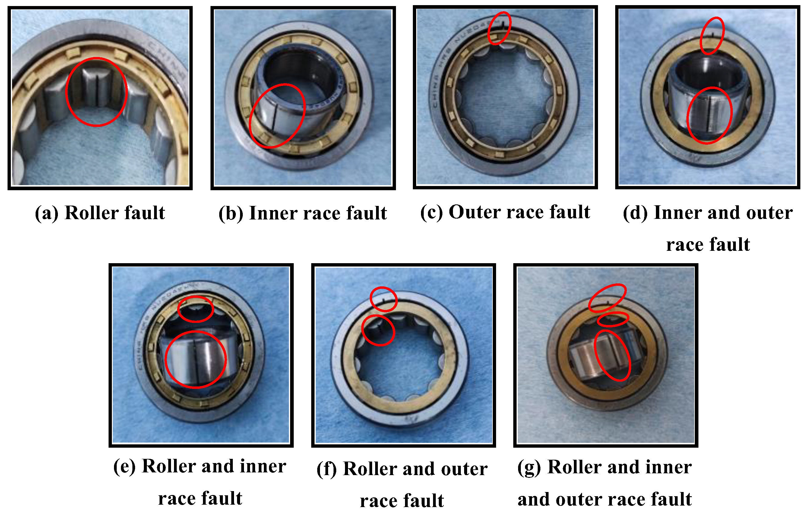
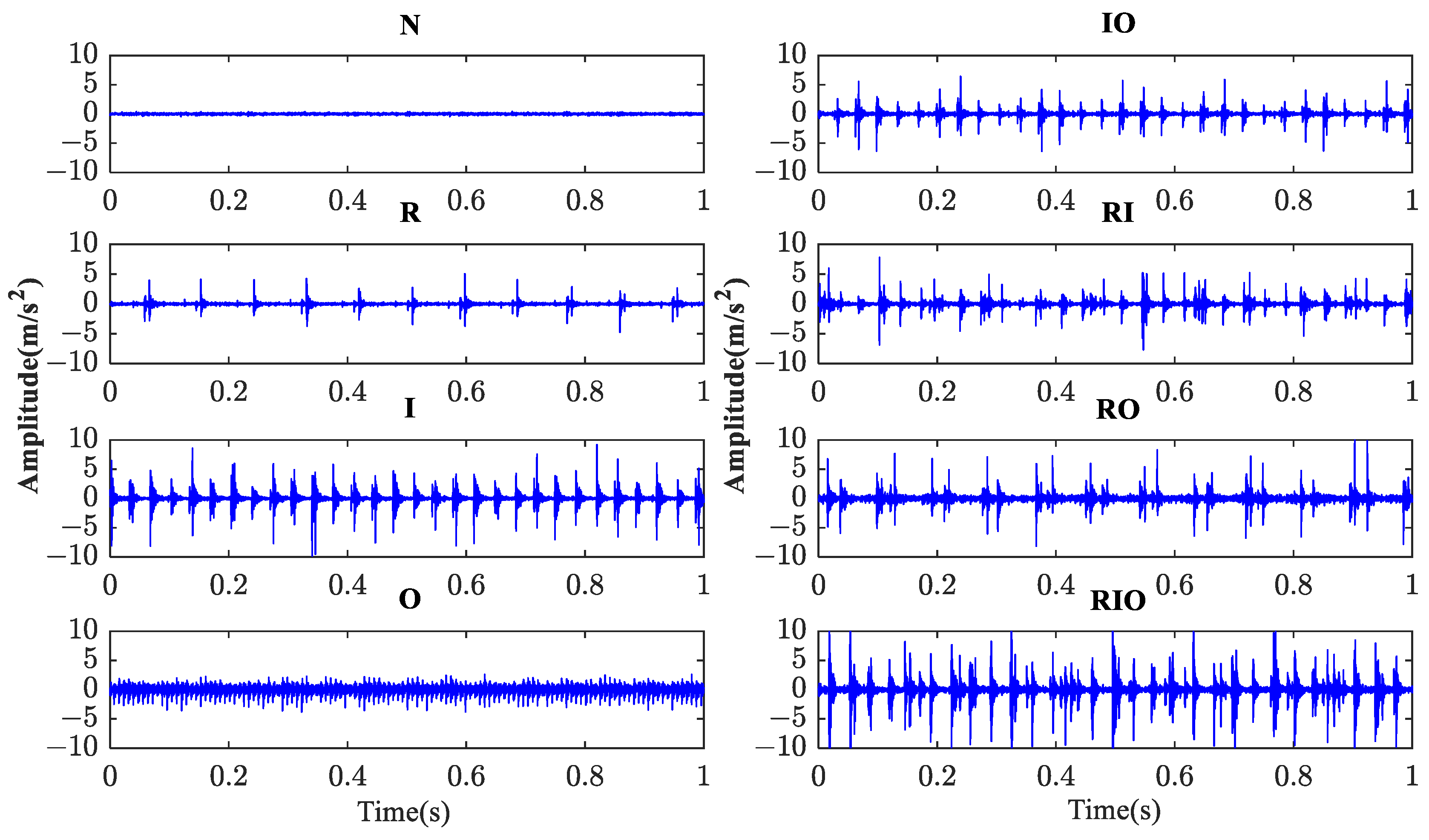
| Bearing State | Abbreviation |
|---|---|
| Normal | N |
| Roller fault | R |
| Inner race fault | I |
| Outer race fault | O |
| Inner and outer race fault | IO |
| Roller and inner race fault | RI |
| Roller and outer race fault | RO |
| Roller and inner and outer race fault | RIO |
| Different Methods | Number of Tests | Mean | SD | Time (s) | |||||||||
|---|---|---|---|---|---|---|---|---|---|---|---|---|---|
| 1 | 2 | 3 | 4 | 5 | 6 | 7 | 8 | 9 | 10 | ||||
| BCMFDE | 99.79% | 99.79% | 100% | 99.79% | 99.79% | 100% | 100% | 99.79% | 99.58% | 99.79% | 99.83% | 0.13% | 91.93 |
| HFDE | 93.75% | 94.58% | 95.21% | 96.46% | 94.38% | 94.79% | 97.08% | 95.63% | 96.04% | 95.83% | 95.37% | 1.02% | 292.82 |
| CMFDE | 99.79% | 99.79% | 100% | 99.79% | 99.58% | 99.79% | 100% | 99.58% | 99.58% | 99.79% | 99.77% | 0.15% | 76.46 |
| MFDE | 97.71% | 97.92% | 97.71% | 96.88% | 97.08% | 97.29% | 97.92% | 98.13% | 97.92% | 96.46% | 97.50% | 0.55% | 8.81 |
| MDE | 96.46% | 96.25% | 97.50% | 96.25% | 96.46% | 96.88% | 97.08% | 97.50% | 96.88% | 95.63% | 96.69% | 0.59% | 2.61 |
| MPE | 15.83% | 16.67% | 17.29% | 17.29% | 15.83% | 16.25% | 17.71% | 14.79% | 16.67% | 19.58% | 16.79% | 1.30% | 9.72 |
| MSE | 84.38% | 84.17% | 83.33% | 86.04% | 83.33% | 84.17% | 85.83% | 82.29% | 82.92% | 83.75% | 84.02% | 1.19% | 308.12 |
| Parameter | Value |
|---|---|
| Bearing type | 6205–2RS JEM SKF |
| Pitch diameter | 39.04 (mm) |
| Roller diameter | 7.94 (mm) |
| Number of the roller | 9 |
| Contact angle | 0° |
| Bearing State | Defect Size (mm) | Abbreviation |
|---|---|---|
| Normal | 0 | N |
| Roller fault | 0.18 | R1 |
| Roller fault | 0.36 | R2 |
| Roller fault | 0.53 | R3 |
| Inner race fault | 0.18 | I1 |
| Inner race fault | 0.36 | I2 |
| Inner race fault | 0.53 | I3 |
| Outer race fault | 0.18 | O1 |
| Outer race fault | 0.36 | O2 |
| Outer race fault | 0.53 | O3 |
| Different Methods | Number of Tests | Mean | SD | Time (s) | |||||||||
|---|---|---|---|---|---|---|---|---|---|---|---|---|---|
| 1 | 2 | 3 | 4 | 5 | 6 | 7 | 8 | 9 | 10 | ||||
| BCMFDE | 98.18% | 98.18% | 98.18% | 98.18% | 98.18% | 98.18% | 99.09% | 99.09% | 98.18% | 97.27% | 98.27% | 0.52% | 21.30 |
| HFDE | 94.55% | 92.73% | 93.64% | 95.45% | 92.73% | 96.36% | 90.90% | 95.45% | 93.64% | 95.45% | 94.09% | 1.67% | 54.83 |
| CMFDE | 96.36% | 95.45% | 98.18% | 98.18% | 95.45% | 97.27% | 97.27% | 99.09% | 96.36% | 97.27% | 97.09% | 1.20% | 10.72 |
| MFDE | 94.55% | 95.45% | 94.55% | 94.55% | 95.45% | 96.36% | 98.18% | 95.45% | 96.36% | 93.64% | 95.45% | 1.29% | 1.98 |
| MDE | 93.64% | 91.82% | 90.91% | 91.82% | 92.73% | 96.36% | 98.18% | 91.82% | 88.18% | 90.91% | 92.64% | 2.86% | 0.63 |
| MPE | 19.09% | 20.91% | 19.09% | 19.09% | 18.18% | 24.55% | 20.91% | 23.64% | 19.09% | 19.09% | 20.36% | 2.15% | 2.24 |
| MSE | 79.09% | 80.91% | 80.00% | 82.73% | 80.00% | 81.82% | 84.55% | 85.45% | 82.73% | 80.00% | 81.73% | 2.12% | 71.63 |
Disclaimer/Publisher’s Note: The statements, opinions and data contained in all publications are solely those of the individual author(s) and contributor(s) and not of MDPI and/or the editor(s). MDPI and/or the editor(s) disclaim responsibility for any injury to people or property resulting from any ideas, methods, instructions or products referred to in the content. |
© 2023 by the authors. Licensee MDPI, Basel, Switzerland. This article is an open access article distributed under the terms and conditions of the Creative Commons Attribution (CC BY) license (https://creativecommons.org/licenses/by/4.0/).
Share and Cite
Xue, Z.; Huang, Y.; Zhang, W.; Shi, J.; Luo, H. Intelligent Fault Diagnosis of Rolling Bearings Based on a Complete Frequency Range Feature Extraction and Combined Feature Selection Methodology. Sensors 2023, 23, 8767. https://doi.org/10.3390/s23218767
Xue Z, Huang Y, Zhang W, Shi J, Luo H. Intelligent Fault Diagnosis of Rolling Bearings Based on a Complete Frequency Range Feature Extraction and Combined Feature Selection Methodology. Sensors. 2023; 23(21):8767. https://doi.org/10.3390/s23218767
Chicago/Turabian StyleXue, Zhengkun, Yukun Huang, Wanyang Zhang, Jinchuan Shi, and Huageng Luo. 2023. "Intelligent Fault Diagnosis of Rolling Bearings Based on a Complete Frequency Range Feature Extraction and Combined Feature Selection Methodology" Sensors 23, no. 21: 8767. https://doi.org/10.3390/s23218767
APA StyleXue, Z., Huang, Y., Zhang, W., Shi, J., & Luo, H. (2023). Intelligent Fault Diagnosis of Rolling Bearings Based on a Complete Frequency Range Feature Extraction and Combined Feature Selection Methodology. Sensors, 23(21), 8767. https://doi.org/10.3390/s23218767