

Research on the 3D Reverse Time Migration Technique for Internal Defects Imaging and Sensor Settings of Pressure Pipelines


Abstract
:1. Introduction
2. Materials and Methods
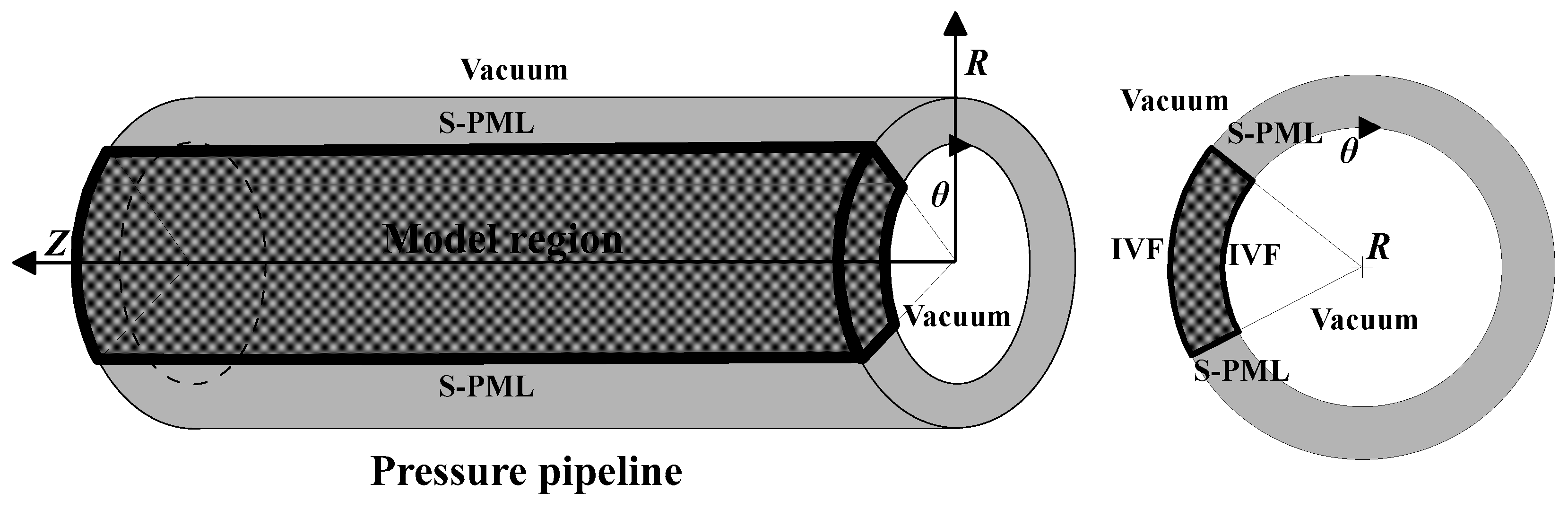
2.1. Extrapolation of the Wave-Field in Cylindrical Coordinates
2.2. Boundary Conditions
2.3. Imaging Condition
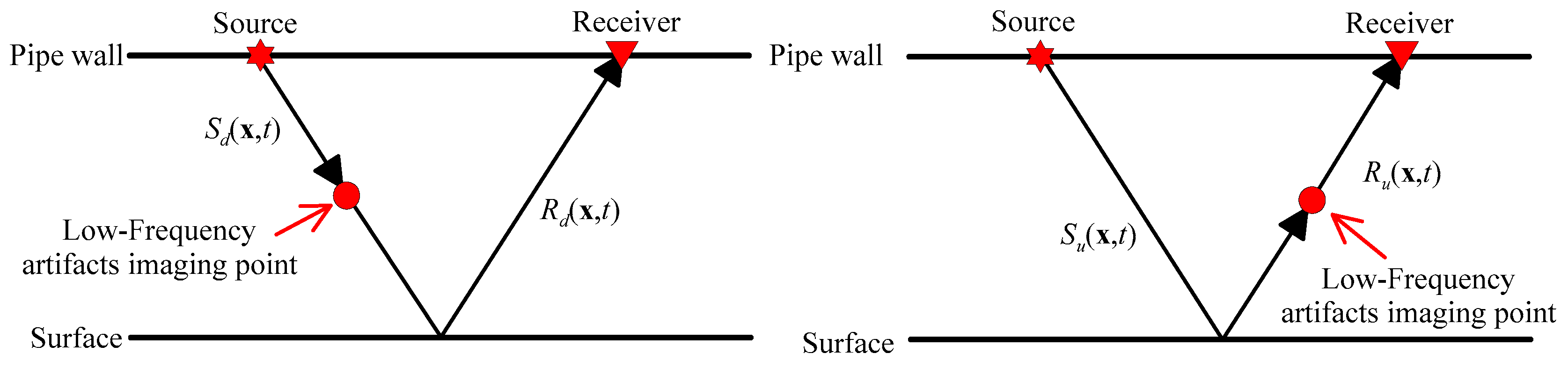
2.4. RTM Artifacts
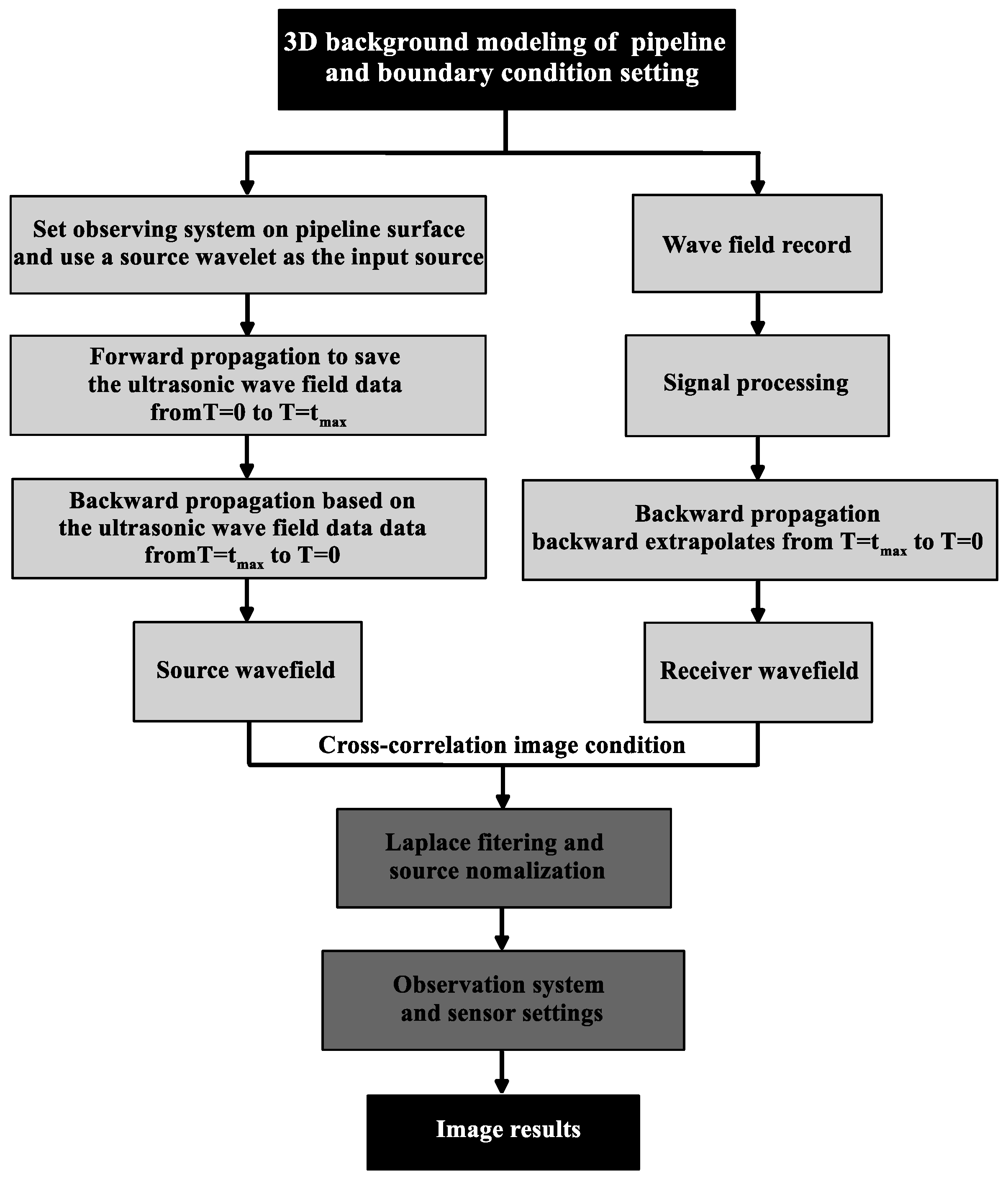
2.5. Implementation
3. Numerical Simulation Results and Discussion
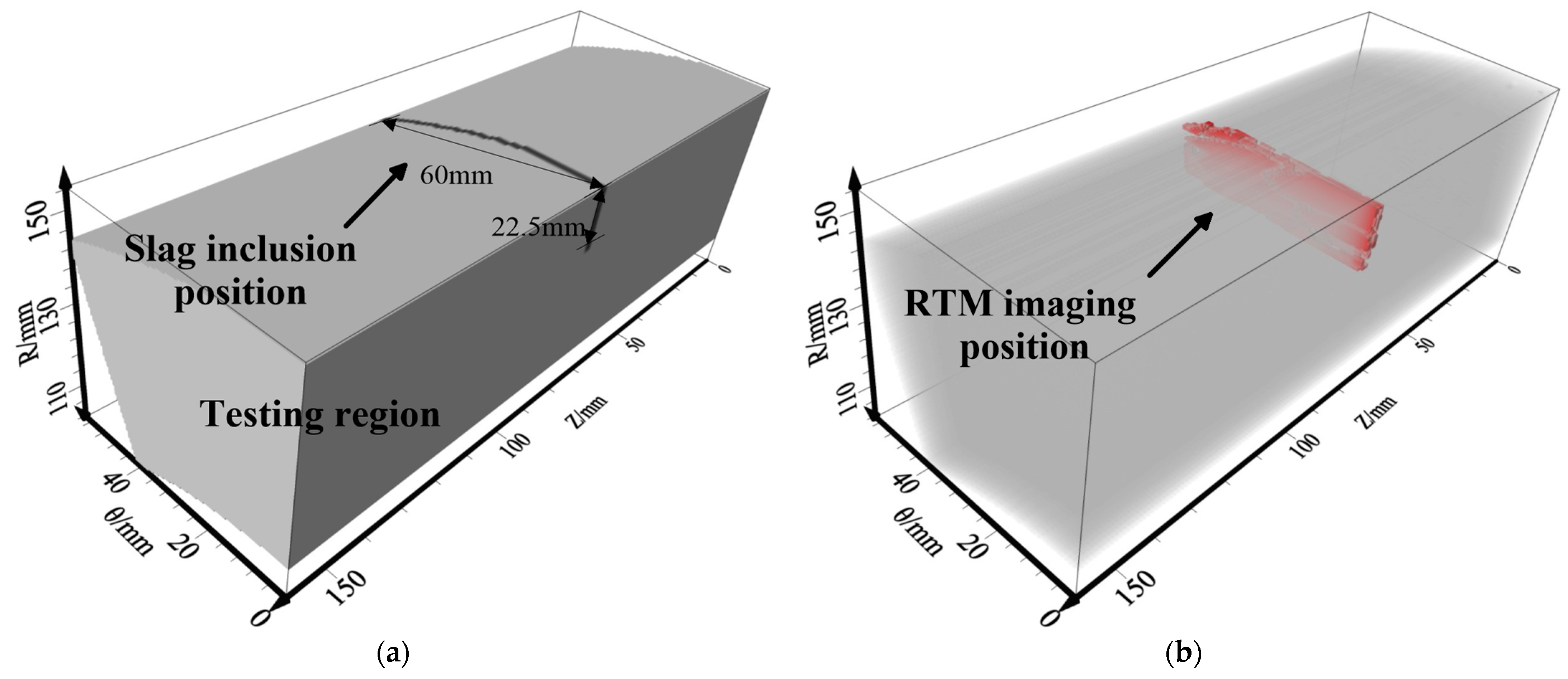
3.1. Survey Design and Modelling
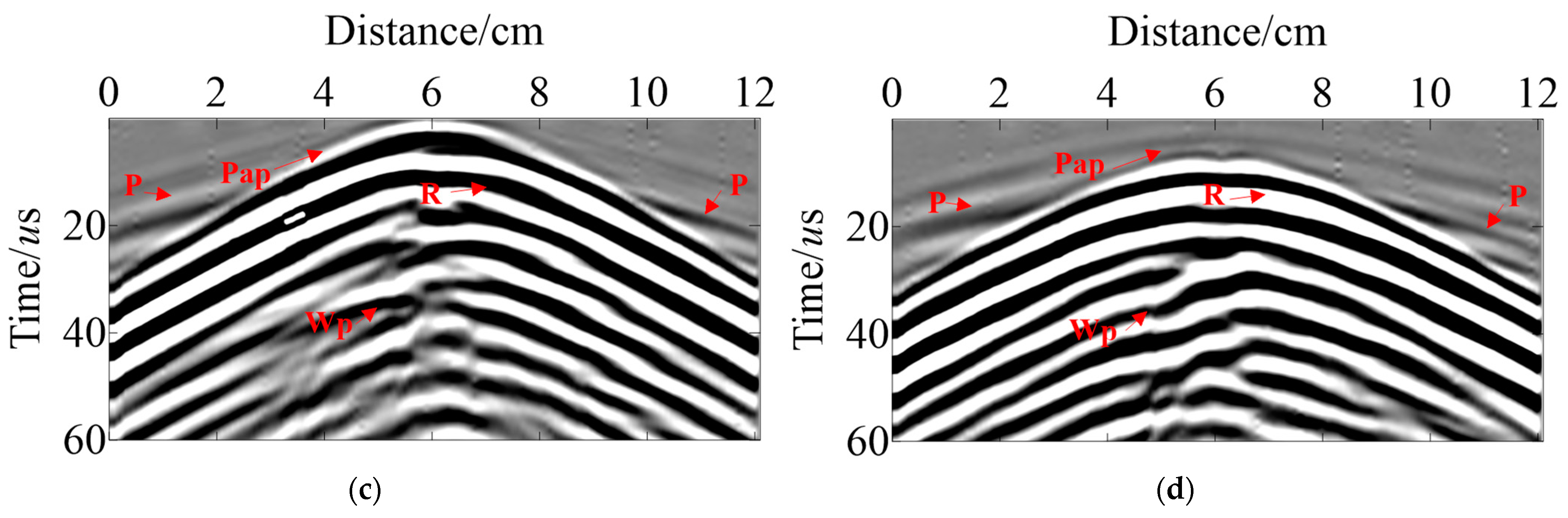
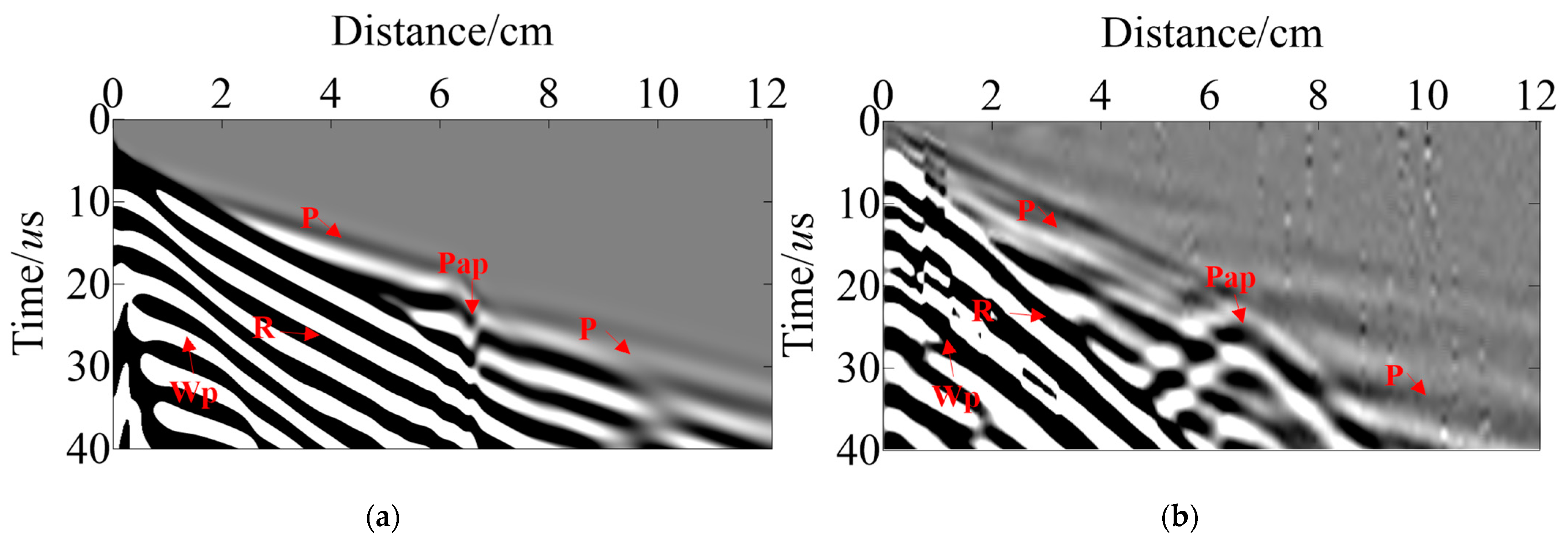
3.2. Wavefield Extrapolation Results
3.2.1. Model-1
3.2.2. Model-2
3.3. RTM Imaging Artifacts Suppression
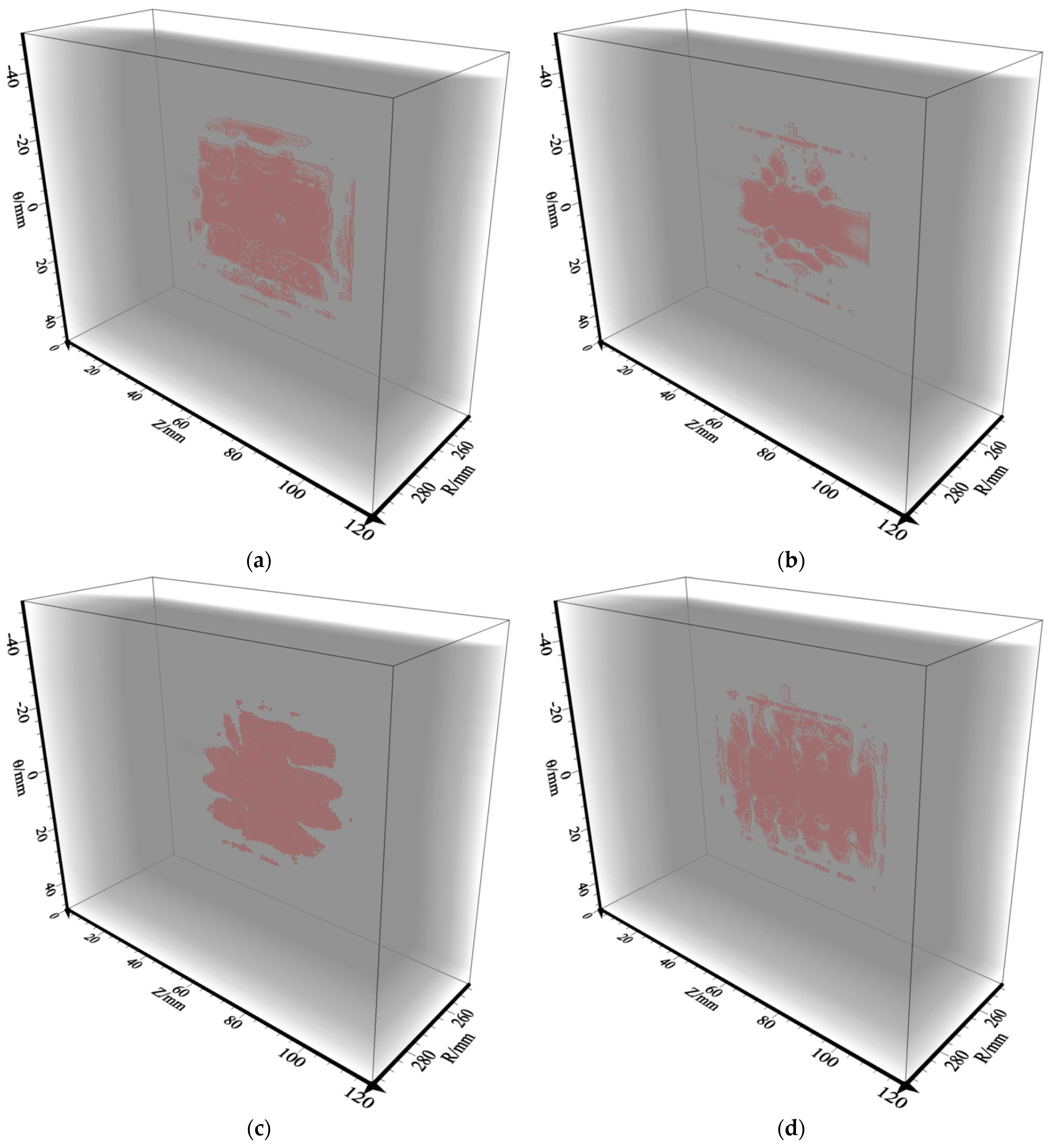
3.4. Sensor Settings and Observation System Discussion
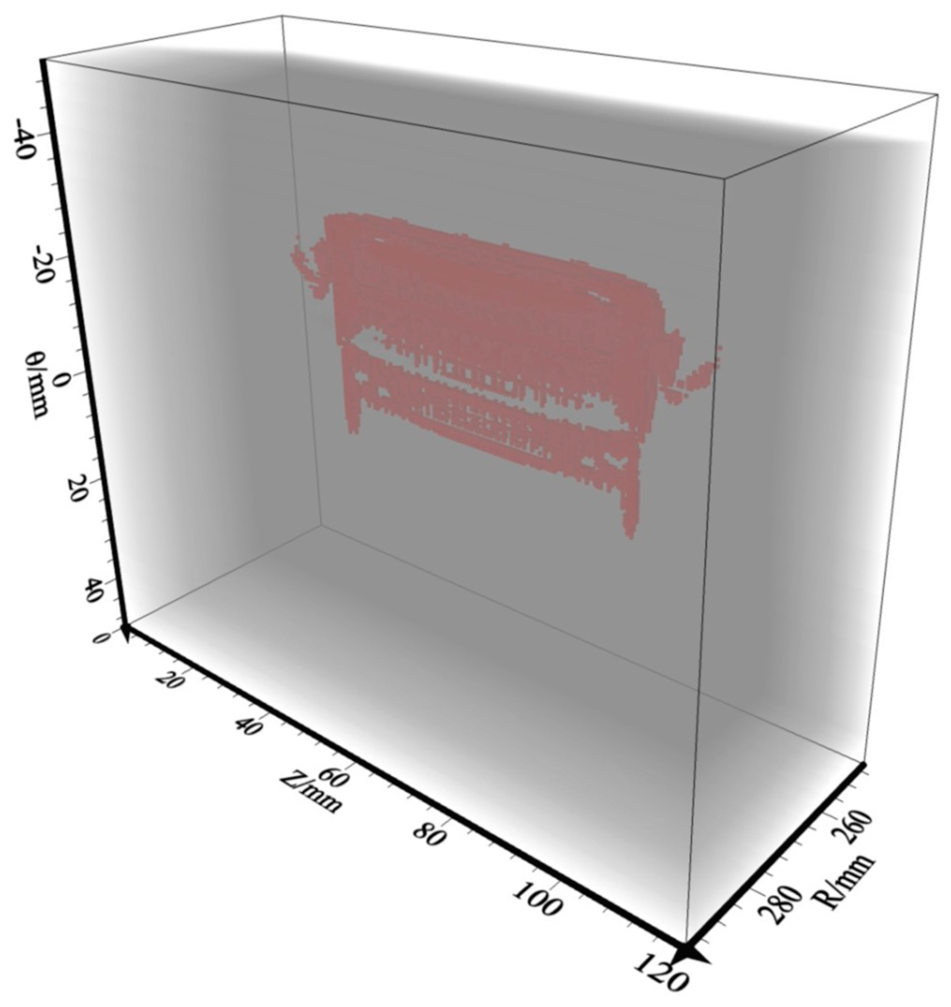
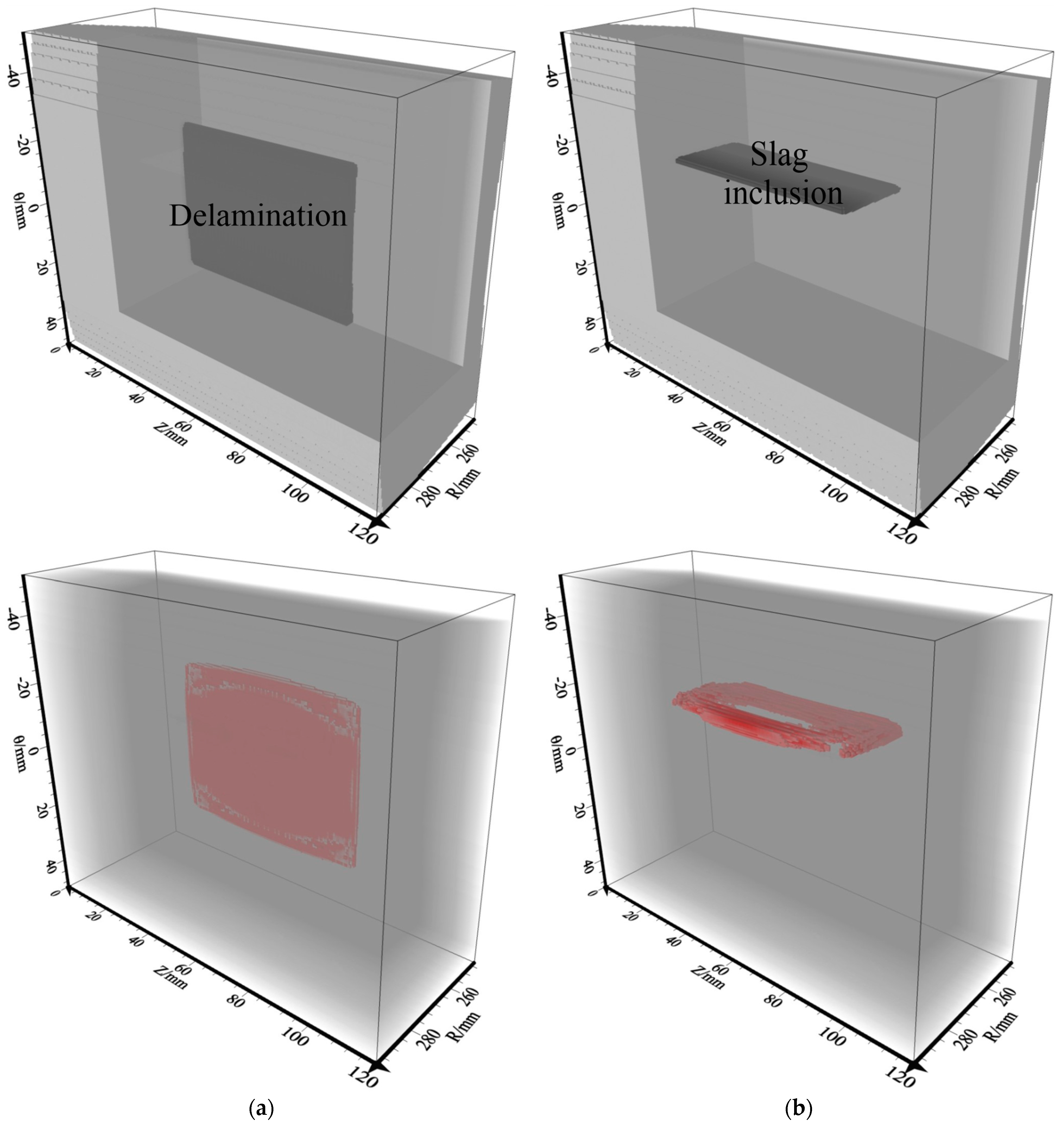
3.5. RTM Imaging Results
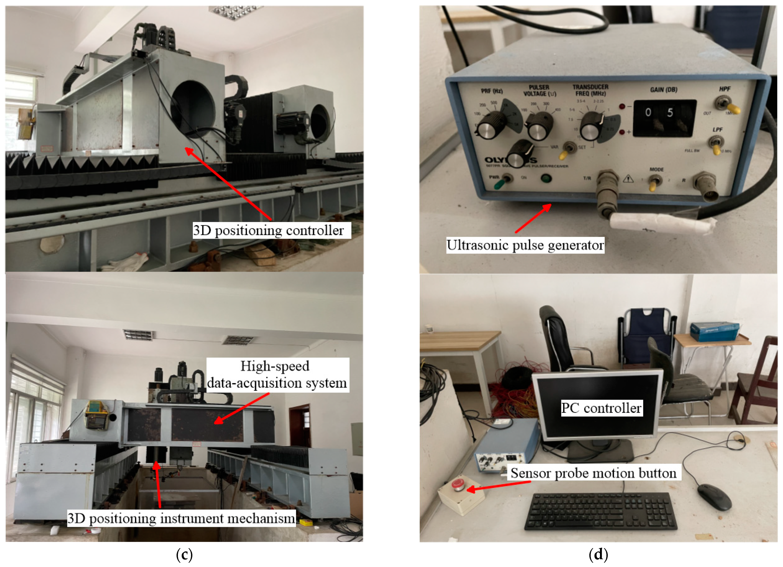
4. Laboratory Experiment Results and Discussion
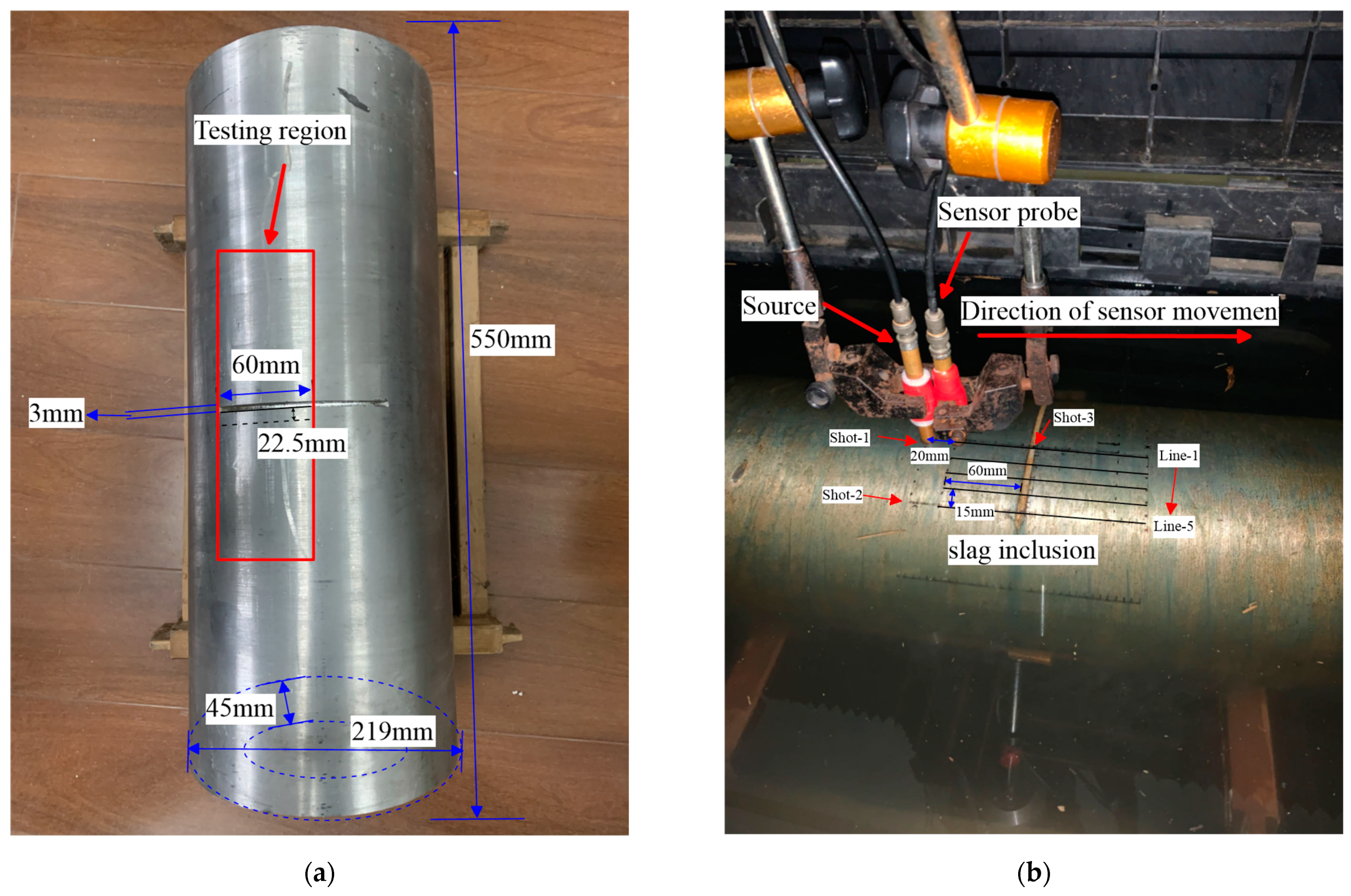
4.1. Specimens and Empirical Setup
4.2. Field Test Results
5. Conclusions
Author Contributions
Funding
Institutional Review Board Statement
Informed Consent Statement
Data Availability Statement
Conflicts of Interest
References
- Du, F.; Li, C.; Wang, W. Development of Subsea Pipeline Buckling, Corrosion and Leakage Monitoring. J. Mar. Sci. Eng. 2023, 11, 188. [Google Scholar] [CrossRef]
- Chang, J.; Wang, C.; Tang, Y.; Li, W. Numerical investigations of ultrasonic reverse time migration for complex cracks near the surface. IEEE Access 2022, 10, 5559–5567. [Google Scholar] [CrossRef]
- Peng, D.; Cheng, F.; She, X.; Zheng, Y.; Tang, Y.; Fan, Z. Three-Dimensional Ultrasonic Reverse-Time Migration Imaging of Submarine Pipeline Nonde-structive Testing in Cylindrical Coordinates. J. Mar. Sci. Eng. 2023, 11, 1459. [Google Scholar] [CrossRef]
- Sheng, H.; Wang, P. Evaluation of Pipeline Steel Mechanical Property Distribution Based on Multimicromagnetic NDT Method. IEEE Trans. Instrum. Meas. 2023, 72, 6001715. [Google Scholar] [CrossRef]
- Rifai, D.; Abdalla, A.N.; Razali, R.; Ali, K.; Faraj, M.A. An eddy current testing platform system for pipe defect inspection based on an optimized eddy current technique probe design. Sensors 2017, 17, 579. [Google Scholar] [CrossRef] [PubMed]
- Nasraoui, S.; Louati, M.; Ghidaoui, M.S. Blockage detection in pressurized water-filled pipe using high frequency acoustic waves. Mech. Syst. Signal Process. 2023, 185, 109817. [Google Scholar] [CrossRef]
- Boaretto, N.; Centeno, T.M. Automated detection of welding defects in pipelines from radiographic images DWDI. NDT E Int. 2017, 86, 7–13. [Google Scholar] [CrossRef]
- Ross, R.; Baji, A.; Barnett, D. Inner profile measurement for pipes using penetration testing. Sensors 2019, 19, 237. [Google Scholar] [CrossRef]
- Shipway, N.; Huthwaite, P.; Lowe, M.; Barden, T. Using ResNets to perform automated defect detection for Fluorescent Penetrant Inspection. NDT E Int. 2021, 119, 102400. [Google Scholar] [CrossRef]
- Chen, Y.; Feng, B.; Kang, Y.; Liu, B.; Wang, S.; Duan, Z. A novel thermography-based dry magnetic particle testing method. IEEE Trans. Instrum. Meas. 2022, 71, 9505309. [Google Scholar] [CrossRef]
- She, S.; Chen, Y.; He, Y.; Zhou, Z.; Zou, X. Optimal design of remote field eddy current testing probe for ferromagnetic pipeline inspection. Measurement 2021, 168, 108306. [Google Scholar] [CrossRef]
- Suyama, F.M.; Delgado, M.R.; da Silva, R.D.; Centeno, T.M. Deep neural networks based approach for welded joint detection of oil pipelines in radiographic images with Double Wall Double Image exposure. NDT E Int. 2019, 105, 46–55. [Google Scholar] [CrossRef]
- Felice, M.V.; Fan, Z. Sizing of flaws using ultrasonic bulk wave testing: A review. Ultrasonics 2018, 88, 26–42. [Google Scholar] [CrossRef]
- Vogelaar, B.; Golombok, M. Quantification and localization of internal pipe damage. Mech. Syst. Signal Process. 2016, 78, 107–117. [Google Scholar] [CrossRef]
- Rao, J.; Tao, Y.; Sun, Y.; Miao, C.; Wang, W. Detection of defects in highly attenuating materials using ultrasonic least-squares reverse time mi-gration with preconditioned stochastic gradient descent. Ultrasonics 2023, 131, 106930. [Google Scholar] [CrossRef] [PubMed]
- De Simone, M.E.; Boccardi, S.; Fierro, G.P.M.; Meo, M. Nonlinear Ultrasonic Imaging for Porosity Evaluation. Sensors 2023, 23, 6319. [Google Scholar] [CrossRef]
- Hong, J.; Choi, H. Monitoring hardening behavior of cementitious materials using contactless ultrasonic method. Sensors 2021, 21, 3421. [Google Scholar] [CrossRef]
- Zhu, W.; Xiang, Y.; Zhang, H.; Zhang, M.; Fan, G.; Zhang, H. Super-resolution ultrasonic Lamb wave imaging based on sign coherence factor and total focusing method. Mech. Syst. Signal Process. 2023, 190, 3421. [Google Scholar] [CrossRef]
- Chen, R.; Tran, K.T.; La, H.M.; Rawlinson, T.; Dinh, K. Detection of delamination and rebar debonding in concrete structures with ultrasonic SH-waveform tomography. Autom. Constr. 2022, 133, 104004. [Google Scholar] [CrossRef]
- Wu, C.; Xu, G.; Shan, Y.; Fan, X.; Zhang, X.; Liu, Y. Defect Detection Algorithm for Wing Skin with Stiffener Based on Phased-Array Ultrasonic Imaging. Sensors 2023, 23, 5788. [Google Scholar] [CrossRef]
- Liu, Z.-Y.; Zhang, P.; Zhang, B.-X.; Wang, W. Multi Spherical Wave Imaging Method Based on Ultrasonic Array. Sensors 2022, 22, 6800. [Google Scholar] [CrossRef] [PubMed]
- Bai, Z.; Chen, S.; Jia, L.; Zeng, Z. Phased array ultrasonic signal compressive detection in low-pressure turbine disc. NDT E Int. 2017, 89, 1–13. [Google Scholar] [CrossRef]
- Holmes, C.; Drinkwater, B.W.; Wilcox, P.D. Post-processing of the full matrix of ultrasonic transmit–receive array data for non-destructive evaluation. NDT E Int. 2005, 38, 701–711. [Google Scholar] [CrossRef]
- Mansur Rodrigues Filho, J.F.; Bélanger, P. Probe standoff optimization method for phased array ultrasonic TFM imaging of curved parts. Sensors 2021, 21, 6665. [Google Scholar] [CrossRef] [PubMed]
- He, H.; Sun, K.; Sun, C.; He, J.; Liang, E.; Liu, Q. Suppressing artifacts in the total focusing method using the directivity of laser ultrasound. Photoacoustics 2023, 31, 100490. [Google Scholar] [CrossRef]
- Langenberg, K.; Berger, M.; Kreutter, T.; Mayer, K.; Schmitz, V. Synthetic aperture focusing technique signal processing. NDT Int. 1986, 19, 177–189. [Google Scholar] [CrossRef]
- Ni, C.Y.; Chen, C.; Ying, K.N.; Dai, L.N.; Yuan, L.; Kan, W.W.; Shen, Z.H. Non-destructive laser-ultrasonic Synthetic Aperture Focusing Technique (SAFT) for 3D visu-alization of defects. Photoacoustics 2021, 22, 100248. [Google Scholar] [CrossRef]
- Zhang, Y.; Li, T.; Chen, H.; Xu, Z.; Li, X.; Du, W.; Liu, Y. Research on Photoacoustic Synthetic Aperture Focusing Technology Imaging Method of Internal Defects in Cylindrical Components. Sensors 2023, 23, 6803. [Google Scholar] [CrossRef]
- Li, Z.; Wu, T.; Zhang, W.; Gao, X.; Yao, Z.; Li, Y.; Shi, Y. A Study on determining time-of-flight difference of overlapping ultrasonic signal: Wave-transform network. Sensors 2020, 20, 5140. [Google Scholar] [CrossRef]
- Jin, S.J.; Zhang, B.; Sun, X.; Lin, L. Reduction of layered dead zone in time-of-flight diffraction (TOFD) for pipeline with spectrum analysis method. J. Nondestruct. Eval. 2021, 40, 48. [Google Scholar] [CrossRef]
- Yang, F.; Shi, D.; Lo, L.-Y.; Mao, Q.; Zhang, J.; Lam, K.-H. Auto-Diagnosis of Time-of-Flight for Ultrasonic Signal Based on Defect Peaks Tracking Model. Remote. Sens. 2023, 15, 599. [Google Scholar] [CrossRef]
- Zhang, Y.; Gao, X.; Zhang, J.; Jiao, J. An Ultrasonic Reverse Time Migration Imaging Method Based on Higher-Order Singular Value Decomposition. Sensors 2022, 22, 2534. [Google Scholar] [CrossRef] [PubMed]
- Rao, J.; Wang, J.; Kollmannsberger, S.; Shi, J.; Fu, H.; Rank, E. Point cloud-based elastic reverse time migration for ultrasonic imaging of components with vertical surfaces. Mech. Syst. Signal Process. 2022, 163, 108144. [Google Scholar] [CrossRef]
- Nguyen, L.T.; Modrak, R.T. Ultrasonic wavefield inversion and migration in complex heterogeneous structures: 2D numerical imaging and nondestructive testing experiments. Ultrasonics 2018, 82, 357–370. [Google Scholar] [CrossRef] [PubMed]
- Müller, S.; Niederleithinger, E.; Bohlen, T. Reverse time migration: A seismic imaging technique applied to synthetic ultrasonic data. Int. J. Geophys. 2012, 2012, 128465. [Google Scholar] [CrossRef]
- Whitmore, N.D. Iterative depth migration by backward time propagation. In SEG Technical Program Expanded Abstracts 1983; Society of Exploration Geophysicists: Houston, TX, USA, 1983; pp. 382–385. [Google Scholar]
- Baysal, E.; Kosloff, D.D.; Sherwood JW, C. Reverse time migration. Geophysics 1983, 48, 1514–1524. [Google Scholar] [CrossRef]
- Chang, W.F.; McMechan, G.A. 3-D elastic prestack, reverse-time depth migration. Geophysics 1994, 59, 597–609. [Google Scholar] [CrossRef]
- Zhu, Z.; Cao, D.; Wu, B.; Yin, X.; Wang, Y. Non-orthogonal beam coordinate system wave propagation and reverse time migration. J. Geophys. Eng. 2019, 16, 1071–1083. [Google Scholar] [CrossRef]
- Yang, X.; Wang, K.; Xu, Y.; Xu, L.; Hu, W.; Wang, H.; Su, Z. A reverse time migration-based multistep angular spectrum approach for ultrasonic imaging of specimens with irregular surfaces. Ultrasonics 2020, 108, 106233. [Google Scholar] [CrossRef]
- Fink, M. Time reversal of ultrasonic fields. I. Basic principles. IEEE Trans. Ultrason. Ferroelectr. Freq. Control. 1992, 39, 555–566. [Google Scholar] [CrossRef]
- Ji, K.; Zhao, P.; Zhuo, C.; Chen, J.; Wang, X.; Gao, S.; Fu, J. Ultrasonic full-matrix imaging of curved-surface components. Mech. Syst. Signal Process. 2022, 181, 109522. [Google Scholar] [CrossRef]
- Yarar, M.L.; Yapar, A. In-Wall Imaging for the Reconstruction of Obstacles by Reverse Time Migration. Sensors 2023, 23, 4456. [Google Scholar] [CrossRef] [PubMed]
- Shragge, J.; Blum, T.E.; van Wijk, K.; Adam, L. Full-wavefield modeling and reverse time migration of laser ultrasound data: A feasibility study. Geophysics 2015, 80, D553–D563. [Google Scholar] [CrossRef]
- Beniwal, S.; Ganguli, A. Defect detection around rebars in concrete using focused ultrasound and reverse time migration. Ultrasonics 2015, 62, 112–125. [Google Scholar] [CrossRef] [PubMed]
- Hu, M.; Chen, S.E.; Pan, D. Reverse time migration based ultrasonic wave detection for concrete structures. In Design, Con-struction, and Maintenance of Bridges; American Society of Civil Engineers: Reston, VA, USA, 2014; pp. 53–60. [Google Scholar]
- Guan, P.; Shao, C.; Jiao, Y.; Zhang, G.; Li, B.; Zhou, J.; Huang, P. 3-D Multi-Component Reverse Time Migration Method for Tunnel Seismic Data. Sensors 2021, 21, 3244. [Google Scholar] [CrossRef] [PubMed]
- Huang, S.; Trad, D. Convolutional Neural-Network-Based Reverse-Time Migration with Multiple Reflections. Sensors 2023, 23, 4012. [Google Scholar] [CrossRef] [PubMed]
- Liu, Q.H. Perfectly matched layers for elastic waves in cylindrical and spherical coordinates. J. Acoust. Soc. Am. 1999, 105, 2075–2084. [Google Scholar] [CrossRef]
- Liu, Q.H.; Sinha, B.K. A 3D cylindrical PML/FDTD method for elastic waves in fluid-filled pressurized boreholes in triaxially stressed formations. Geophysics 2003, 68, 1731–1743. [Google Scholar] [CrossRef]
- Zeng, C.; Xia, J.; Miller, R.D.; Tsoflias, G.P. An improved vacuum formulation for 2D finite-difference modeling of Rayleigh waves including surface topography and internal discontinuities. Geophysics 2012, 77, T1–T9. [Google Scholar] [CrossRef]
- Chattopadhyay, S.; McMechan, G.A. Imaging conditions for prestack reverse-time migration. Geophysics 2008, 73, S81–S89. [Google Scholar] [CrossRef]
- Moradpouri, F.; Moradzadeh, A.; Pestana, R.; Ghaedrahmati, R.; Monfared, M.S. An improvement in wavefield extrapolation and imaging condition to suppress reverse time migration artifacts. Geophysics 2017, 82, S403–S409. [Google Scholar] [CrossRef]
- Yang, R.; Chang, X.; Ling, Y.; Feng, Y.E.; Qu, L. Amplitude-compensated Laplacian filtering of reverse time migration and its application. Geophys. Prospect. 2020, 68, 1089–1096. [Google Scholar] [CrossRef]
 and
and  denotes the differential position of the velocity wave field.
and denotes the differential position of the velocity wave field.
denotes the differential position of the velocity wave field.
and denotes the differential position of the velocity wave field.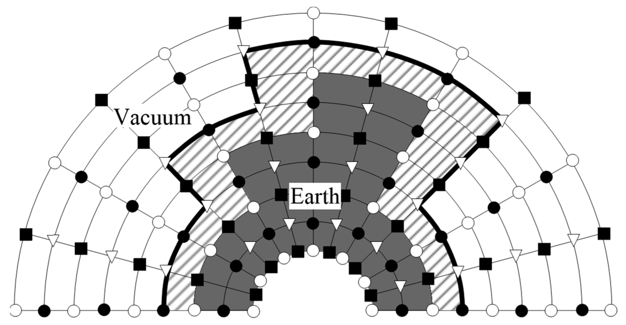


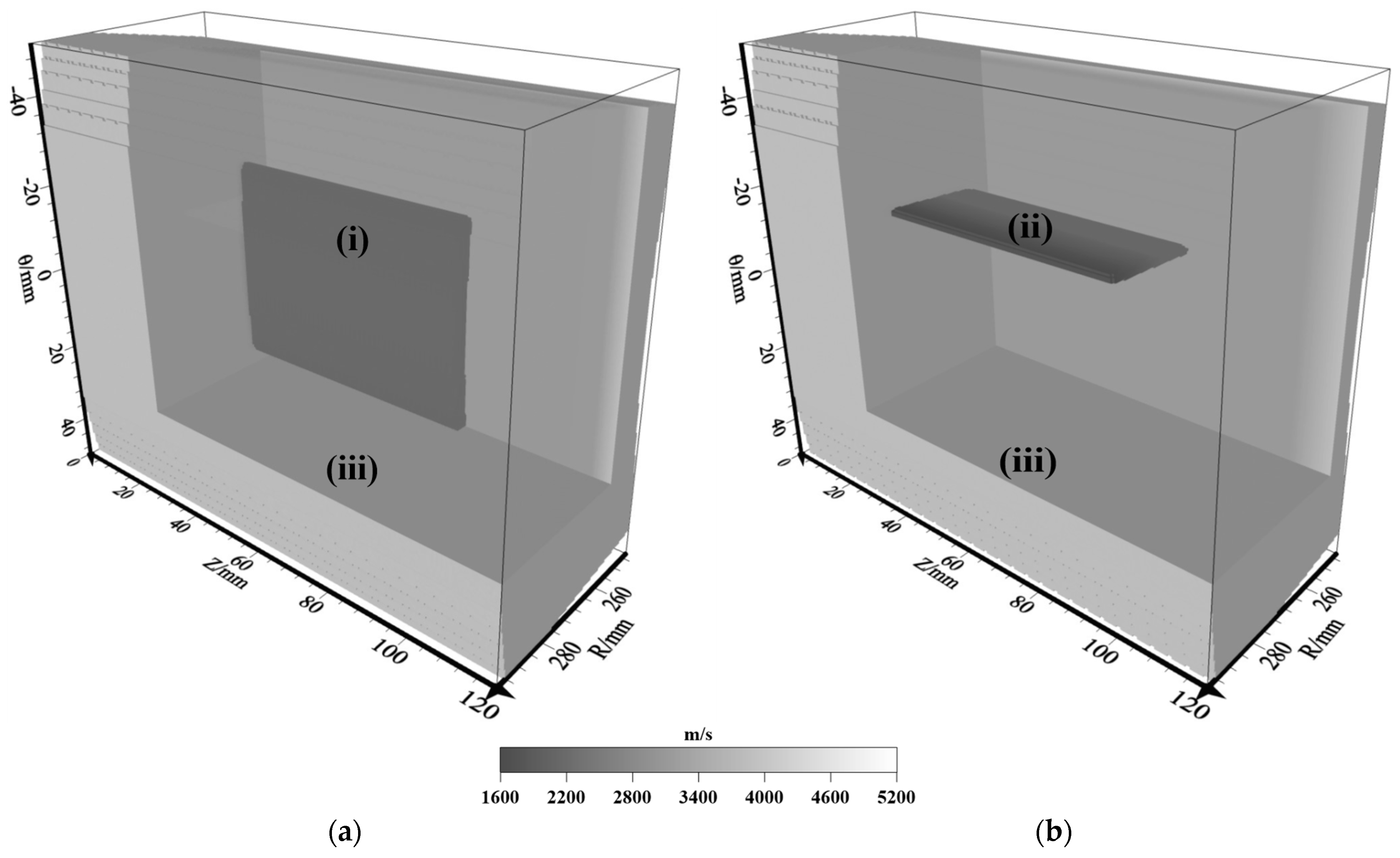
| Medium | Medium Number | ||
|---|---|---|---|
| Delamination defects | (i) | 1733.0 | 3300.0 |
| Slag inclusion defects | (ii) | 1600.0 | 2633.0 |
| Pressure pipelines | (iii) | 5200.0 | 7900.0 |
Disclaimer/Publisher’s Note: The statements, opinions and data contained in all publications are solely those of the individual author(s) and contributor(s) and not of MDPI and/or the editor(s). MDPI and/or the editor(s) disclaim responsibility for any injury to people or property resulting from any ideas, methods, instructions or products referred to in the content. |
© 2023 by the authors. Licensee MDPI, Basel, Switzerland. This article is an open access article distributed under the terms and conditions of the Creative Commons Attribution (CC BY) license (https://creativecommons.org/licenses/by/4.0/).
Share and Cite
Peng, D.; She, X.; Zheng, Y.; Tang, Y.; Fan, Z.; Hu, G. Research on the 3D Reverse Time Migration Technique for Internal Defects Imaging and Sensor Settings of Pressure Pipelines. Sensors 2023, 23, 8742. https://doi.org/10.3390/s23218742
Peng D, She X, Zheng Y, Tang Y, Fan Z, Hu G. Research on the 3D Reverse Time Migration Technique for Internal Defects Imaging and Sensor Settings of Pressure Pipelines. Sensors. 2023; 23(21):8742. https://doi.org/10.3390/s23218742
Chicago/Turabian StylePeng, Daicheng, Xiaoyu She, Yunpeng Zheng, Yongjie Tang, Zhuo Fan, and Guang Hu. 2023. "Research on the 3D Reverse Time Migration Technique for Internal Defects Imaging and Sensor Settings of Pressure Pipelines" Sensors 23, no. 21: 8742. https://doi.org/10.3390/s23218742
APA StylePeng, D., She, X., Zheng, Y., Tang, Y., Fan, Z., & Hu, G. (2023). Research on the 3D Reverse Time Migration Technique for Internal Defects Imaging and Sensor Settings of Pressure Pipelines. Sensors, 23(21), 8742. https://doi.org/10.3390/s23218742