
Acceleration-Based Estimation of Vertical Ground Reaction Forces during Running: A Comparison of Methods across Running Speeds, Surfaces, and Foot Strike Patterns


Abstract
1. Introduction
2. Methods
2.1. IMU Calibration
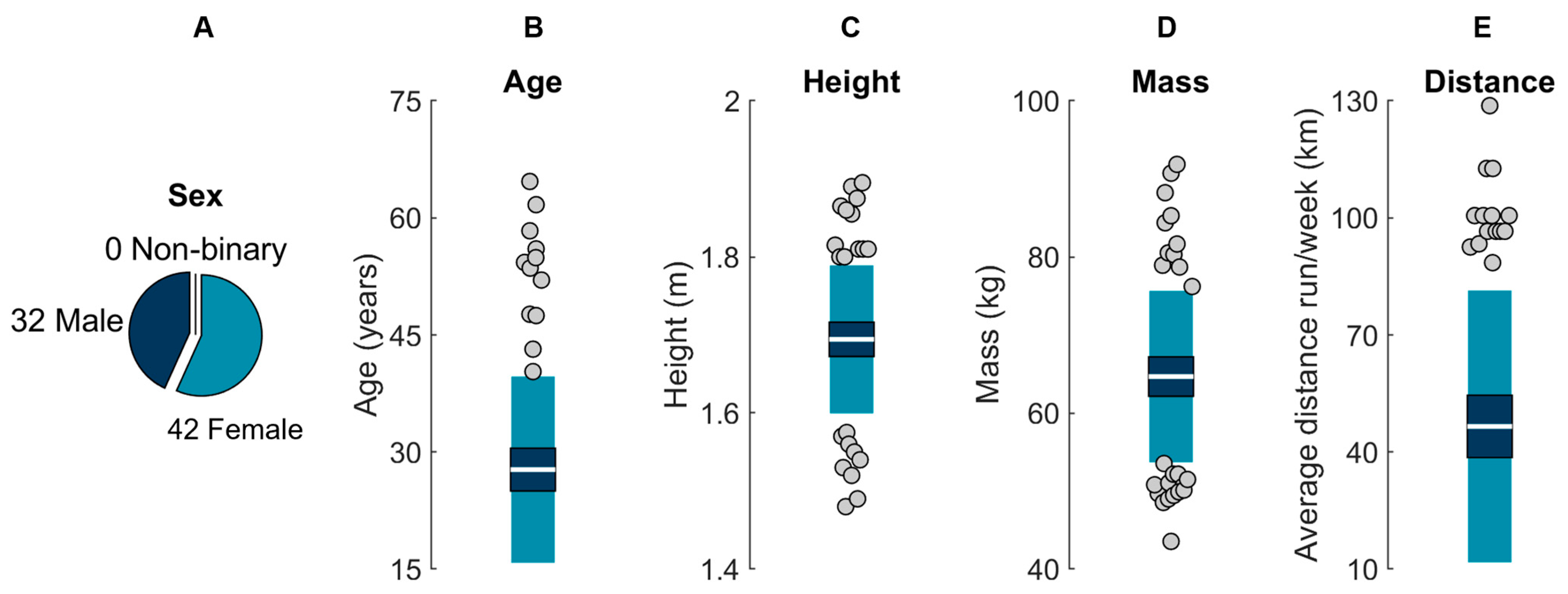
2.2. Participants
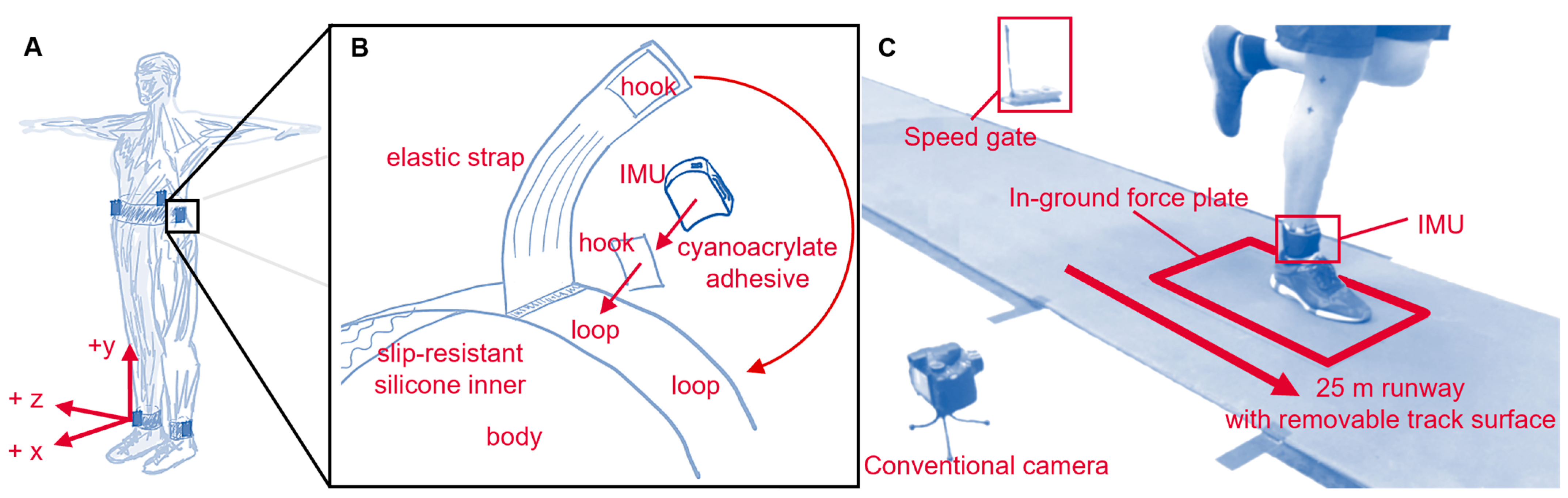
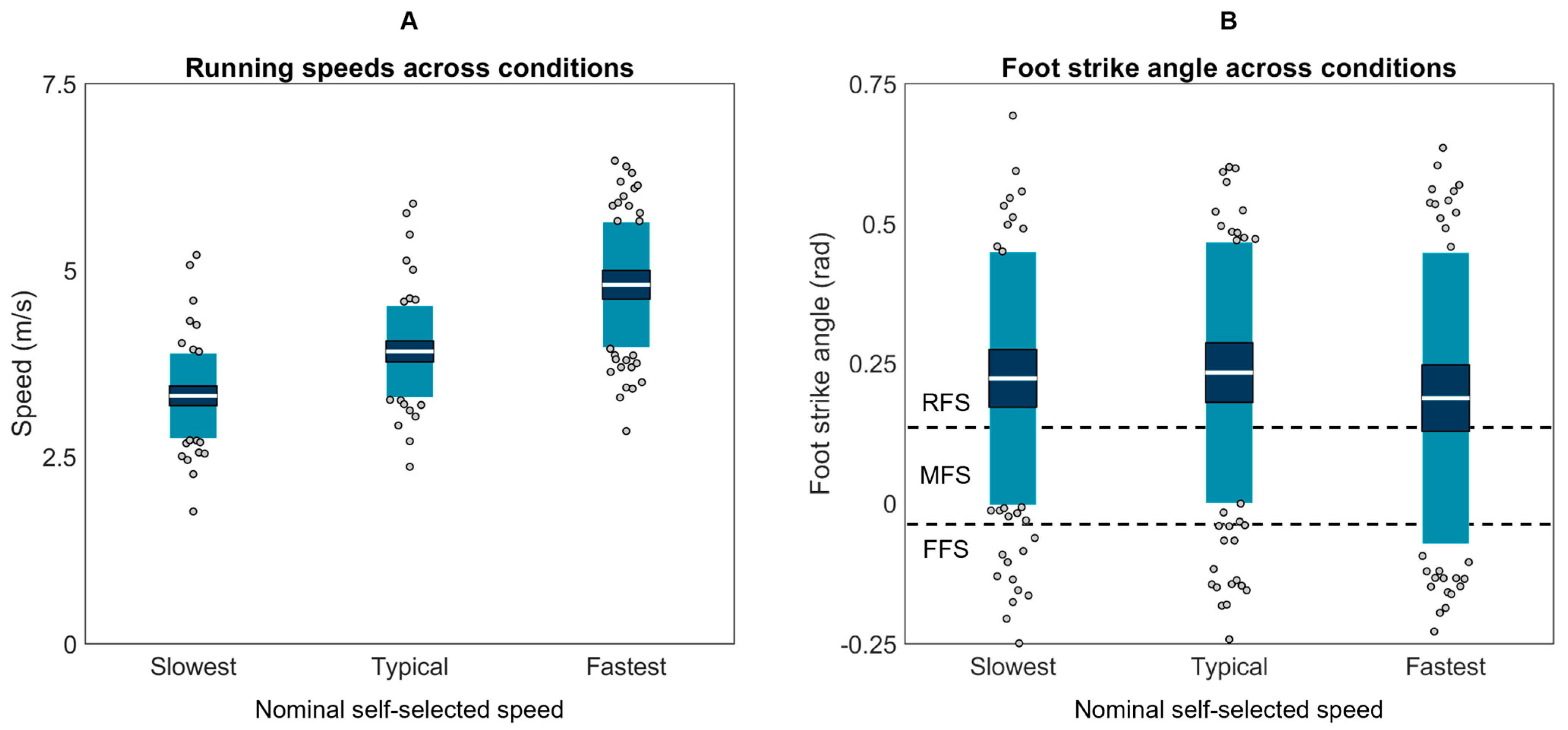
2.3. Protocol
2.4. IMU Data Processing
2.5. Force Data Processing
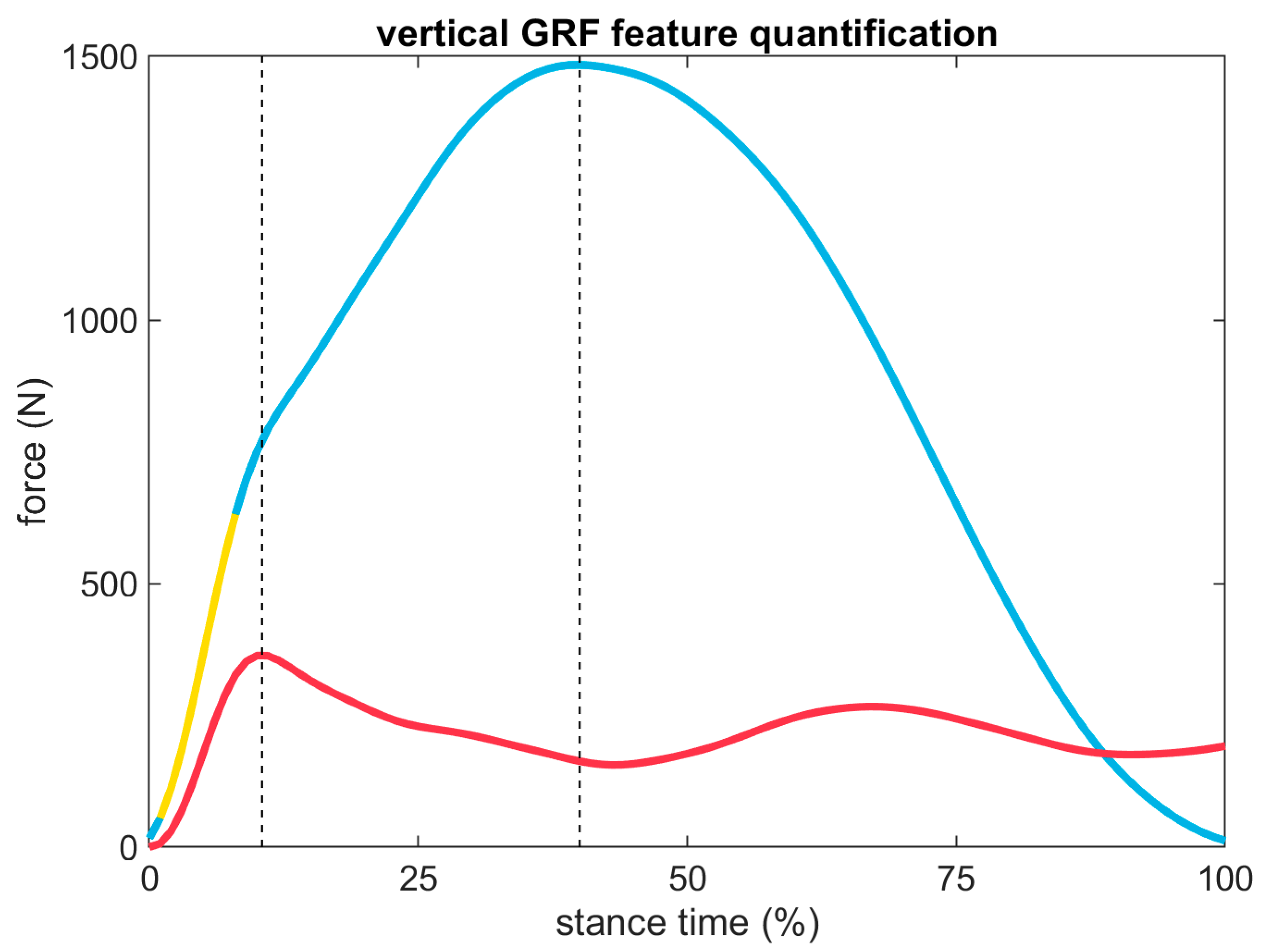
2.6. Analysis
3. Results
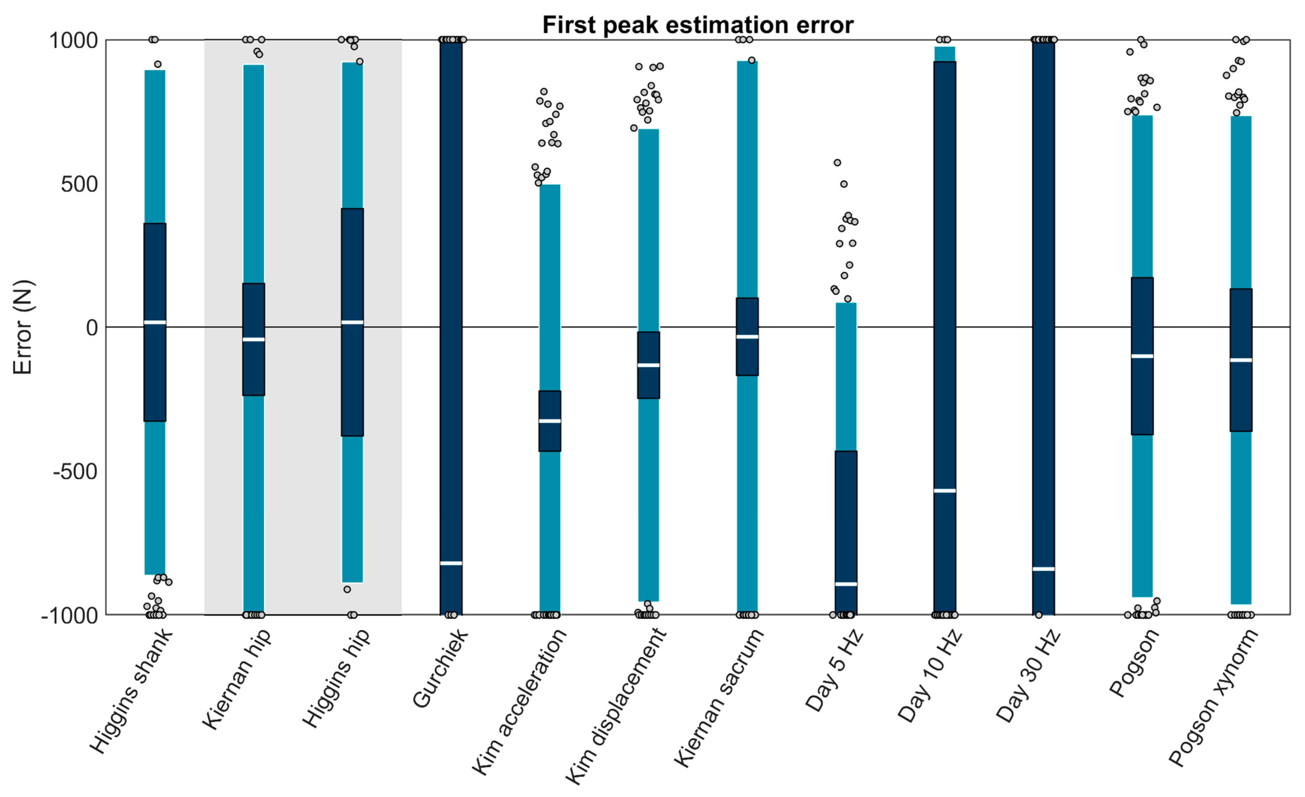
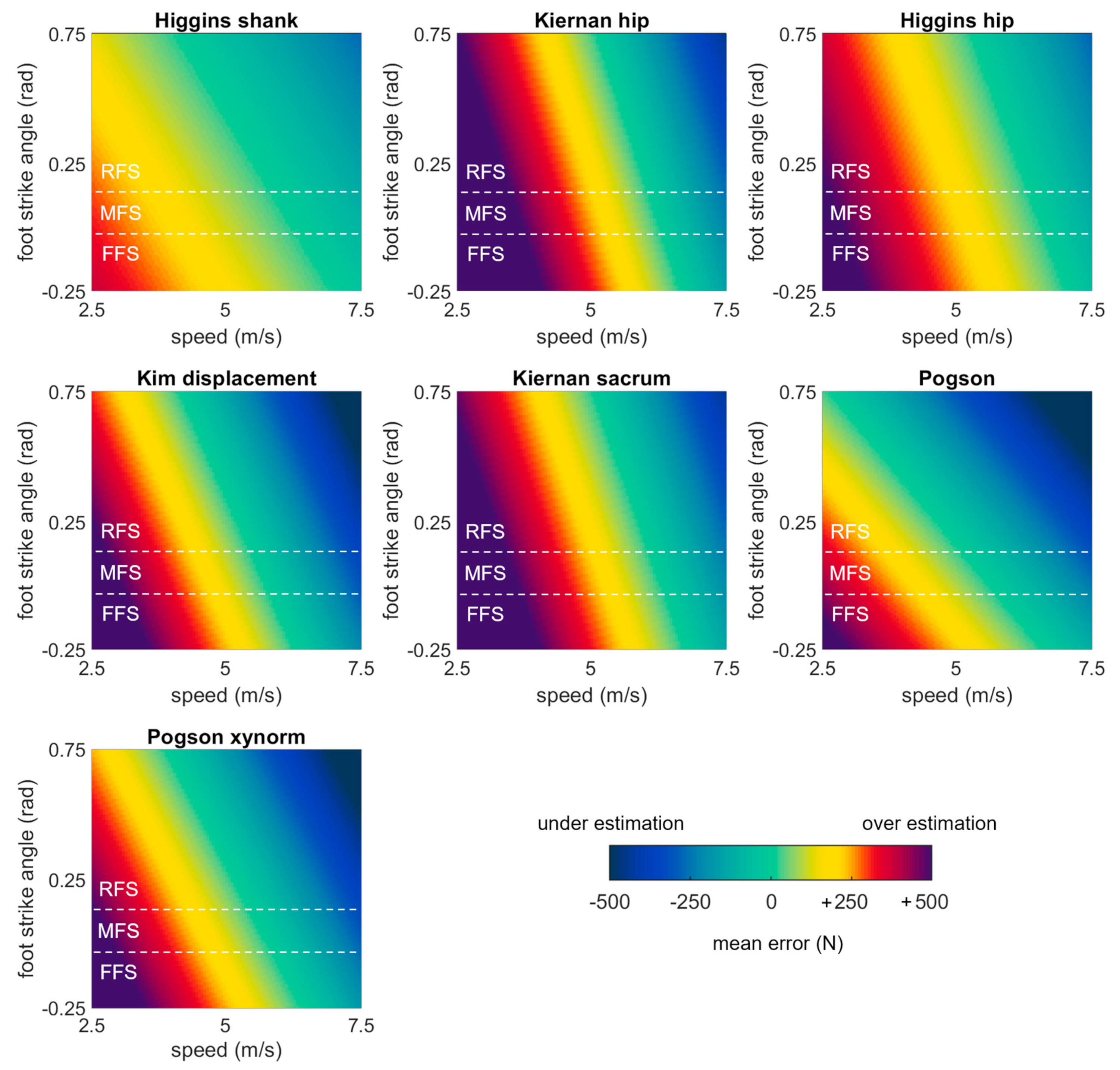
3.1. First Peak
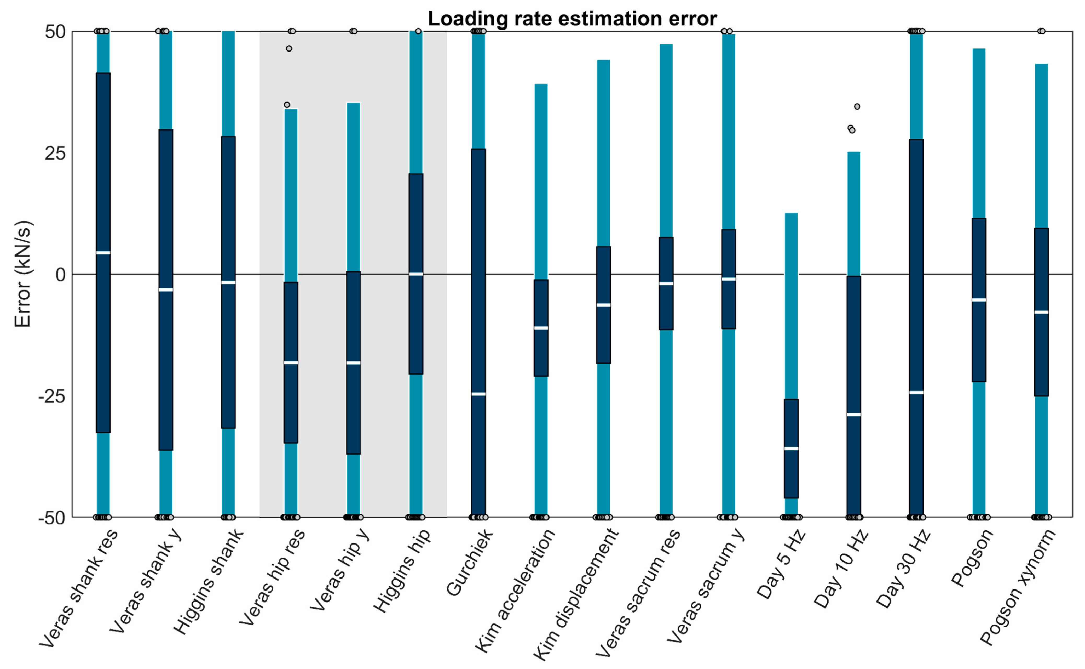
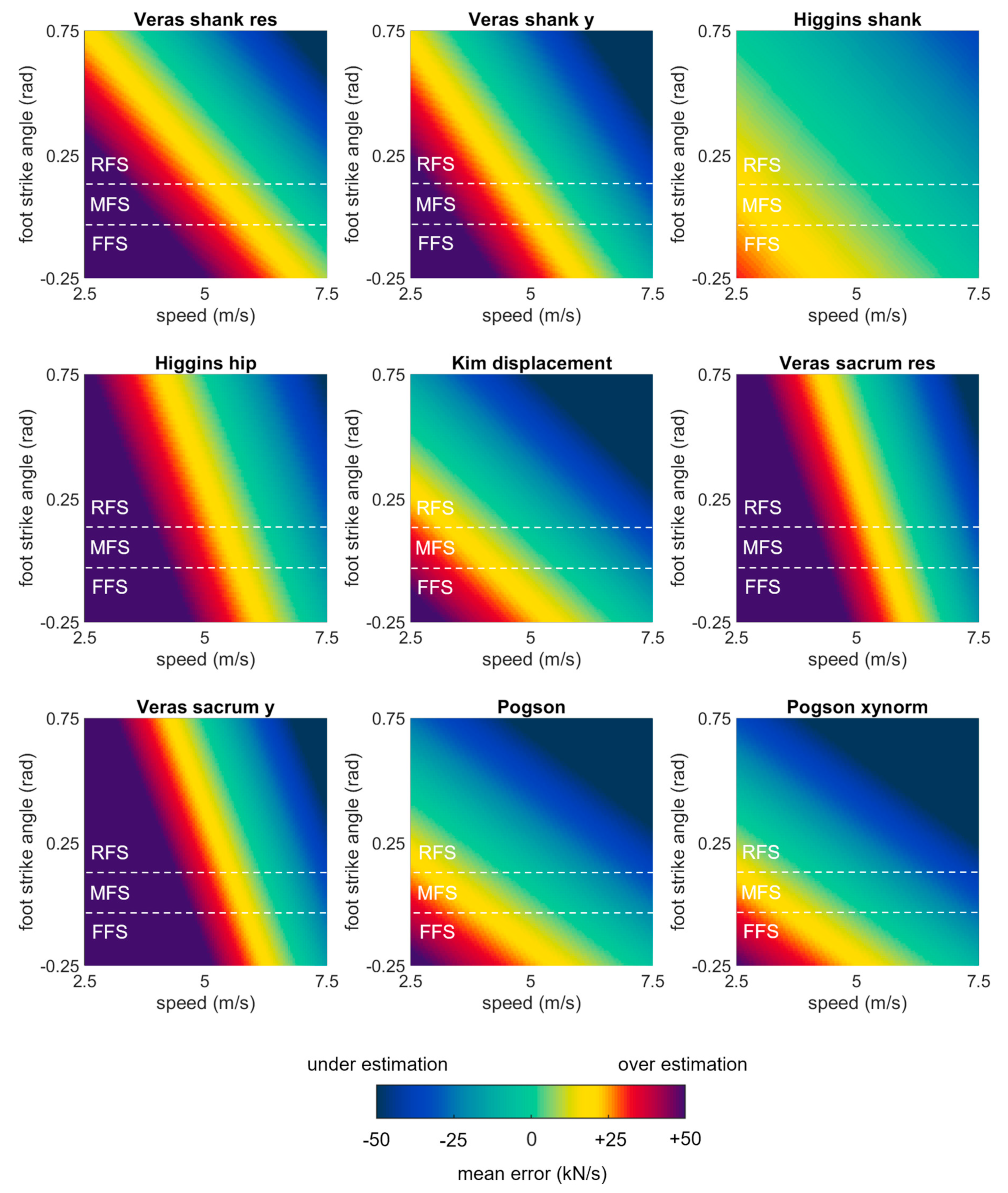
3.2. Loading Rate

| Overall Performance | Performance across Conditions | |||||
|---|---|---|---|---|---|---|
| Method | Bias (kN/s) | RC (kN/s) | LOAs (kN/s) | Speed | Surface | Foot Strike |
| Veras shank res | +4.37 * | 36.96 | 62.56 | −8.28 * | −0.29 | −36.00 * |
| Veras shank y | −3.25 * | 32.96 | 59.96 | −9.14 * | −0.52 | −33.12 * |
| Higgins shank | −1.71 | 29.99 | 56.69 | −3.47 * | 0.92 | −16.17 * |
| Higgins hip | +0.02 | 20.58 | 52.36 | −10.66 * | −0.61 | −21.41 * |
| Kim displacement | −6.34 * | 11.98 | 50.52 | −6.90 * | −1.45 | −37.74 * |
| Veras sacrum res | −1.95 | 9.47 | 49.34 | −12.36 * | −0.96 | −22.08 * |
| Veras sacrum y | −1.04 | 10.18 | 50.52 | −13.83 * | −0.96 | −27.55 * |
| Pogson | −5.32 * | 16.78 | 51.82 | −5.98 * | −1.04 | −40.57 * |
| Pogson xynorm | −7.83 * | 17.25 | 51.21 | −5.99 * | −1.03 | −42.16 * |
 | ||||||

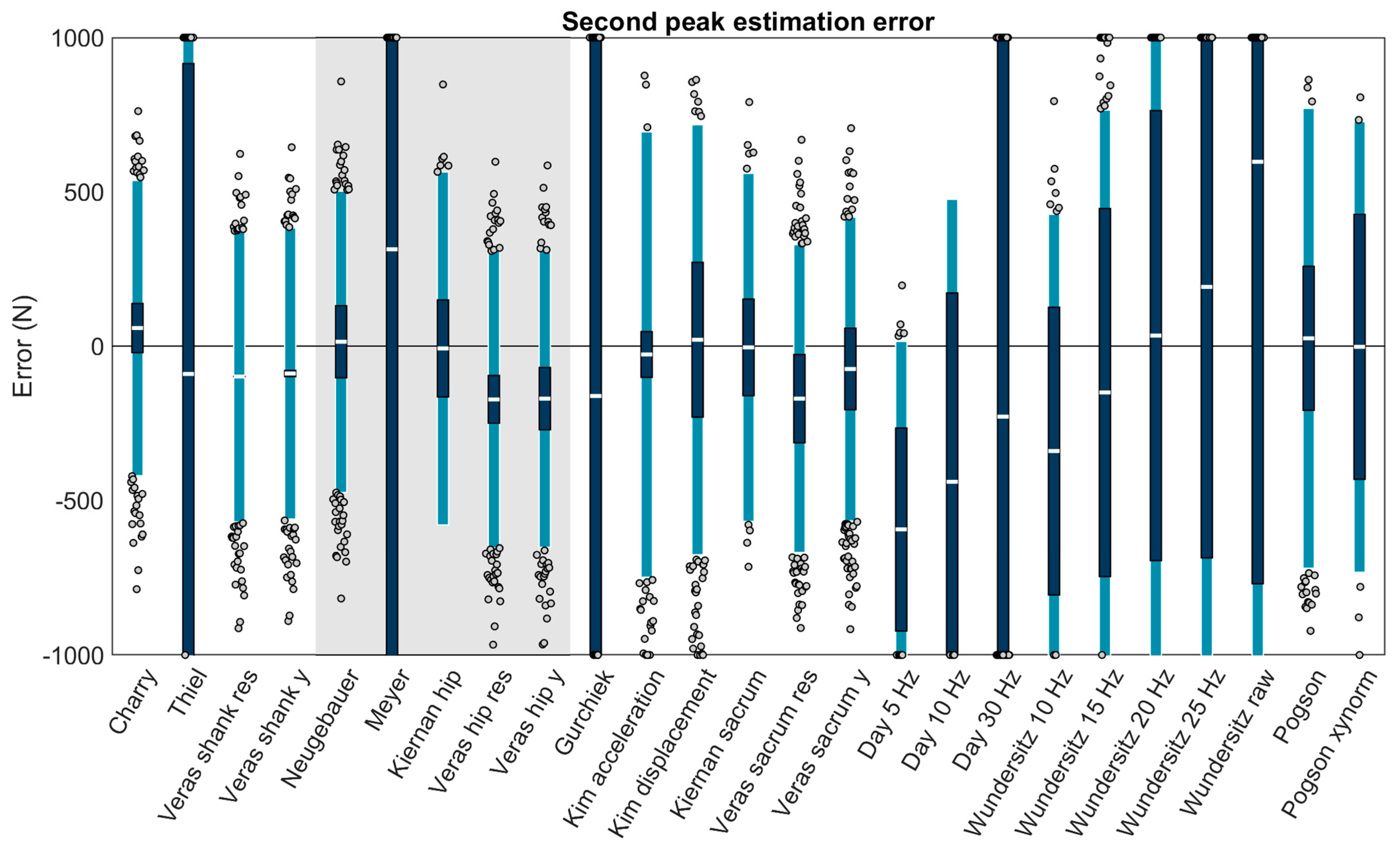
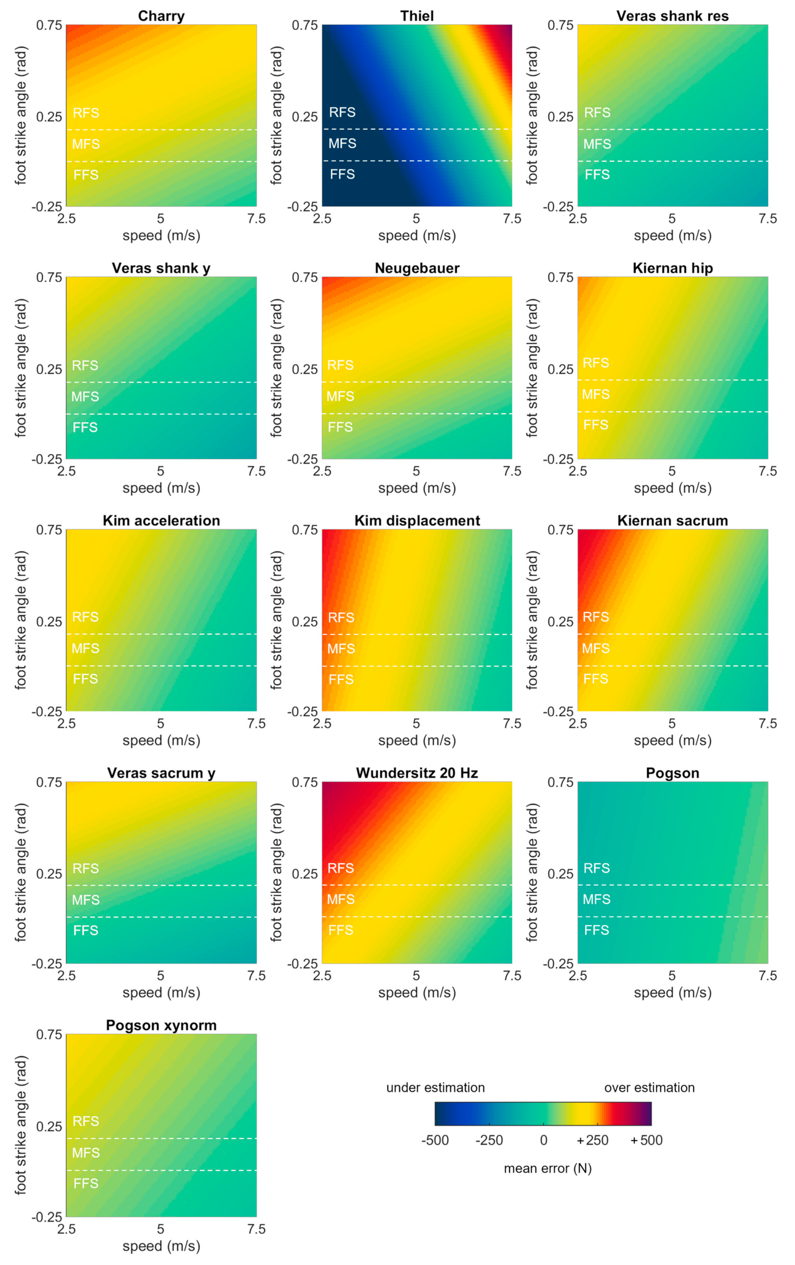
3.3. Second Peak
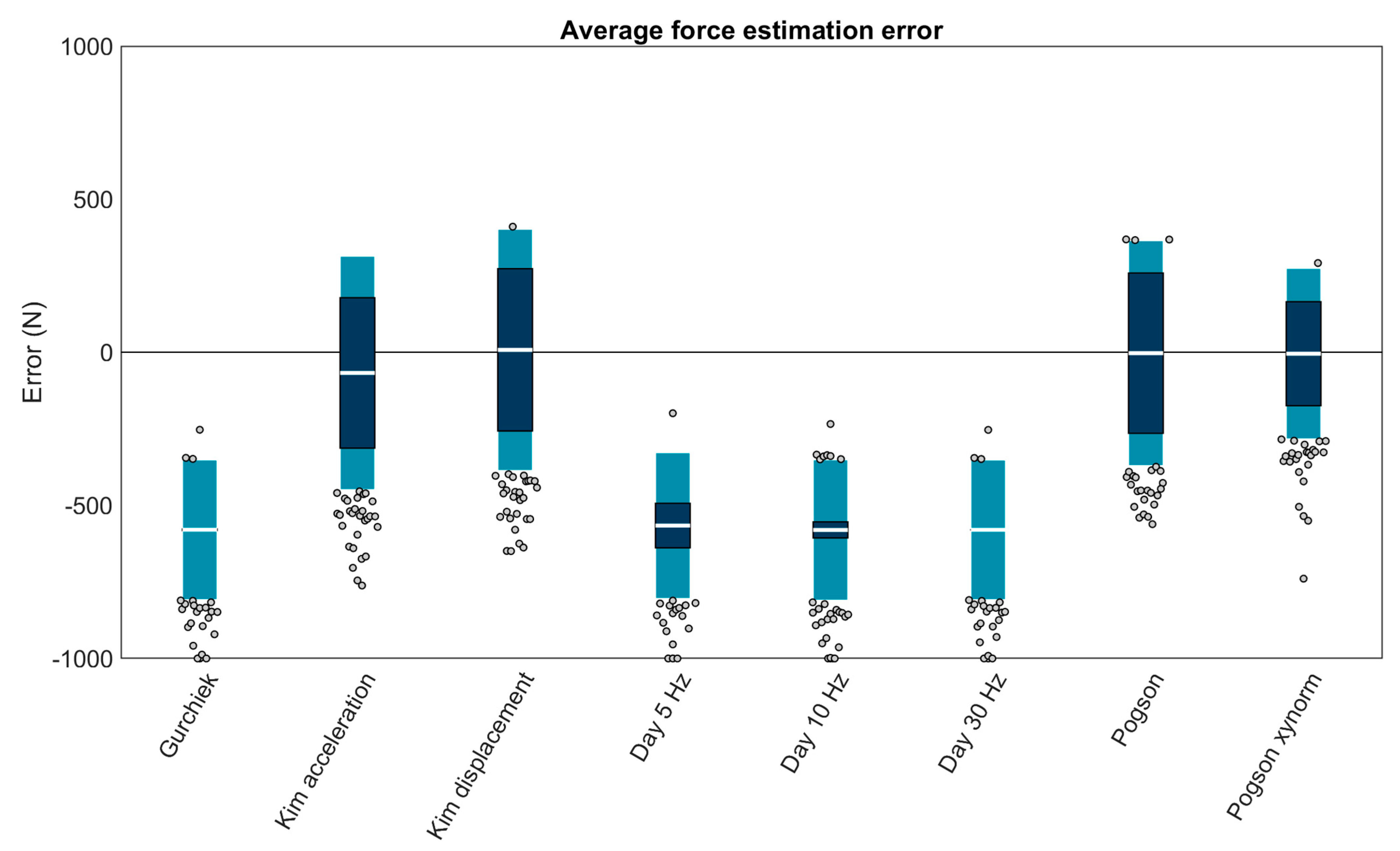
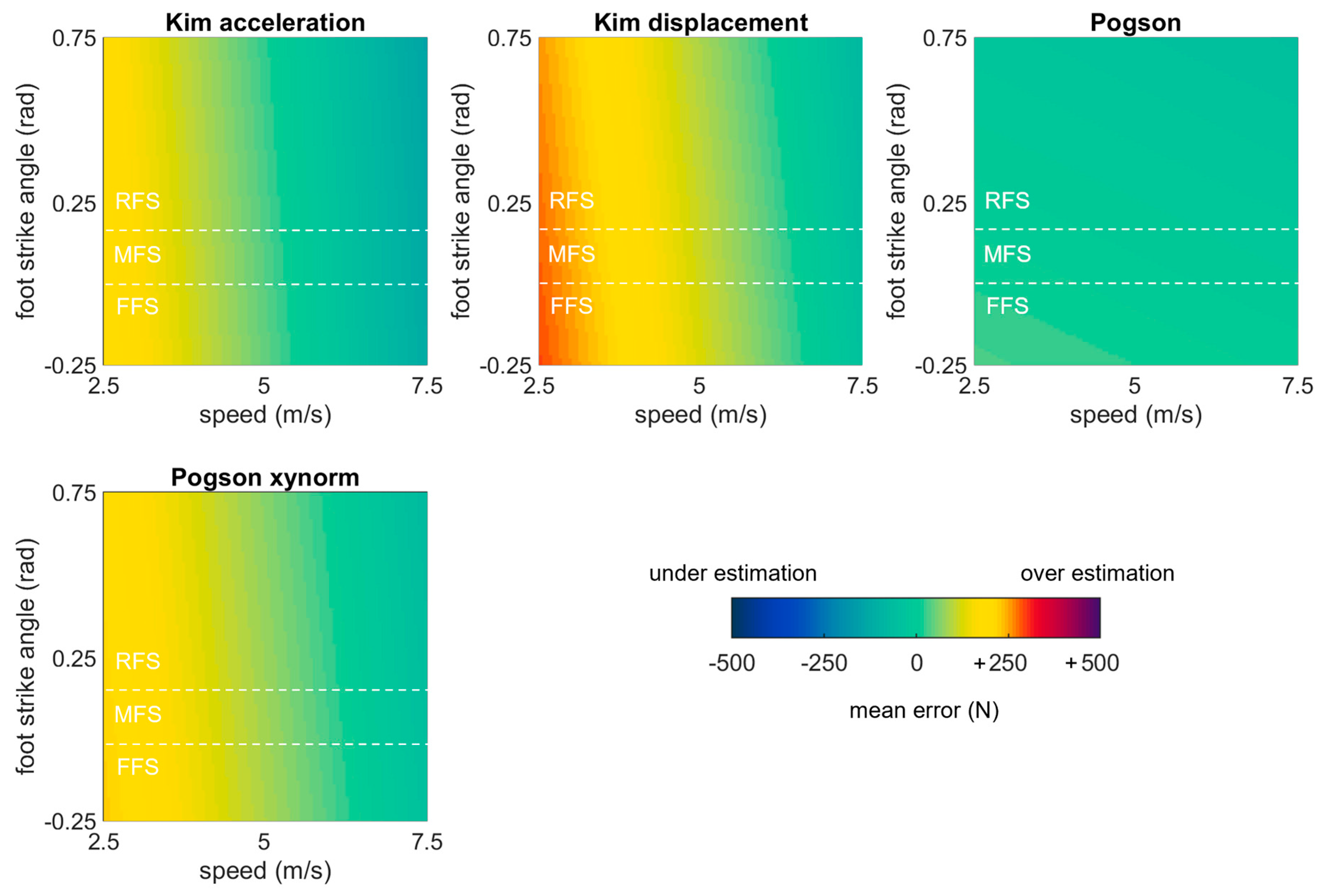
3.4. Average Force
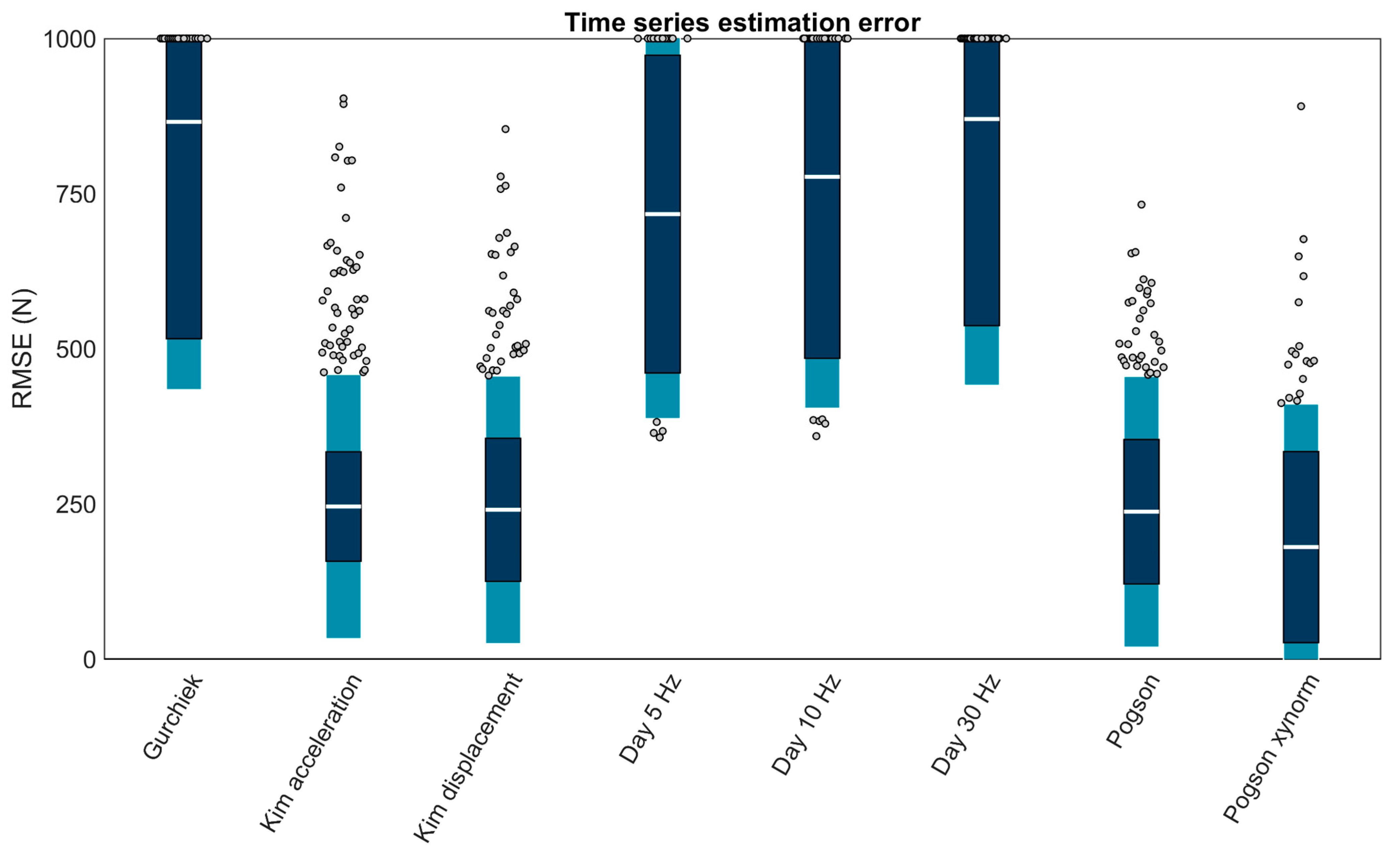
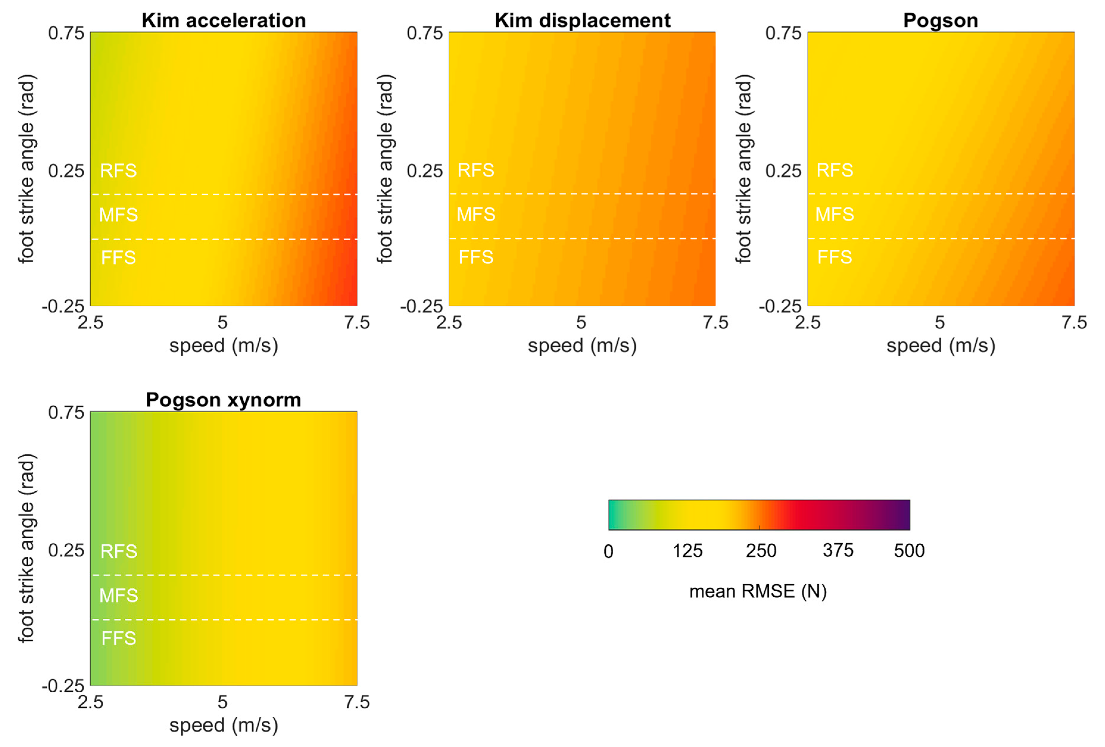
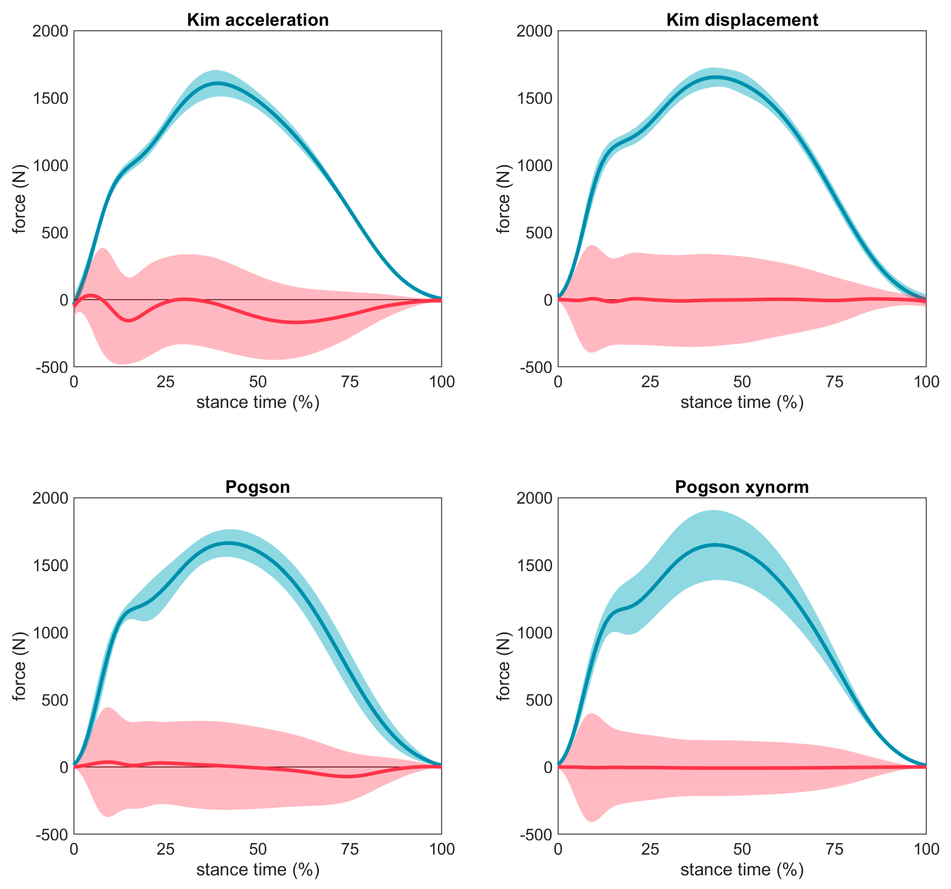
3.5. Time Series
4. Discussion
5. Conclusions and Practical Applications
Supplementary Materials
Author Contributions
Funding
Institutional Review Board Statement
Informed Consent Statement
Data Availability Statement
Conflicts of Interest
References
- Nigg, B.M.; Liu, W. The effect of muscle stiffness and damping on simulated impact force peaks during running. J. Biomech. 1999, 32, 849–856. [Google Scholar] [CrossRef]
- Bredeweg, S.W.; Kluitenberg, B.; Bessem, B.; Buist, I. Differences in kinetic variables between injured and noninjured novice runners: A prospective cohort study. J. Sci. Med. Sport 2013, 16, 205–210. [Google Scholar]
- Crossley, K.; Bennell, K.L.; Wrigley, T.; Oakes, B.W. Ground reaction forces, bone characteristics, and tibial stress fracture in male runners. Med. Sci. Sport. Exerc. 1999, 31, 1088–1093. [Google Scholar] [CrossRef]
- van der Worp, H.; Vrielink, J.W.; Bredeweg, S.W. Do runners who suffer injuries have higher vertical ground reaction forces than those who remain injury free? A systematic review and meta-analysis. Br. J. Sports Med. 2016, 50, 450–457. [Google Scholar]
- Zadpoor, A.A.; Nikooyan, A.A.; Kottner, J.; Black, J.; Call, E.; Gefen, A.; Santamaria, N. The relationship between lower extremity stress fractures and the ground reaction force: A systematic review. Clin. Biomech. 2011, 26, 23–28. [Google Scholar]
- Malisoux, L.; Gette, P.; Delattre, N.; Urhausen, A.; Theisen, D. Spatiotemporal and Ground-Reaction Force Characteristics as Risk Factors for Running-Related Injury: A Secondary Analysis of a Randomized Trial Including 800+ Recreational Runners. Am. J. Sports Med. 2022, 50, 537–544. [Google Scholar] [CrossRef] [PubMed]
- Kiernan, D.; Hawkins, D.A.; Manoukian, M.A.; McKallip, M.; Oelsner, L.; Caskey, C.F.; Coolbaugh, C.L. Accelerometer-based prediction of running injury in National Collegiate Athletic Association track athletes. J. Biomech. 2018, 73, 201–209. [Google Scholar] [CrossRef] [PubMed]
- Ceyssens, L.; Vanelderen, R.; Barton, C.; Malliaras, P.; Dingenen, B. Biomechanical Risk Factors Associated with Running-Related Injuries: A Systematic Review. Sports Med. 2019, 49, 1095–1115. [Google Scholar] [CrossRef] [PubMed]
- Pohl, M.B.; Hamill, J.; Davis, I.S. Biomechanical and anatomic factors associated with a history of plantar fasciitis in female runners. Clin. J. Sport Med. 2009, 19, 372–376. [Google Scholar] [PubMed]
- Kuhman, D.J.; Paquette, M.R.; Peel, S.A.; Melcher, D.A. Comparison of ankle kinematics and ground reaction forces between prospectively injured and uninjured collegiate cross country runners. Hum. Mov. Sci. 2016, 47, 9–15. [Google Scholar] [CrossRef]
- Nagahara, R.; Mizutani, M.; Matsuo, A.; Kanehisa, H.; Fukunaga, T. Association of Sprint Performance With Ground Reaction Forces During Acceleration and Maximal Speed Phases in a Single Sprint. J. Appl. Biomech. 2016, 34, 104–110. [Google Scholar] [CrossRef]
- Morin, J.-B.; Slawinski, J.; Dorel, S.; de Villareal, E.S.; Couturier, A.; Samozino, P.; Brughelli, M.; Rabita, G. Acceleration capability in elite sprinters and ground impulse: Push more, brake less? J. Biomech. 2015, 48, 3149–3154. [Google Scholar] [CrossRef]
- GRabita, G.; Dorel, S.; Slawinski, J.; Sàez-De-Villarreal, E.; Couturier, A.; Samozino, P.; Morin, J.-B. Sprint mechanics in world-class athletes: A new insight into the limits of human locomotion. Scand. J. Med. Sci. Sports 2015, 25, 583–594. [Google Scholar] [CrossRef] [PubMed]
- Dos’Santos, T.; Thomas, C.; Jones, P.A.; Comfort, P. Mechanical Determinants of Faster Change of Direction Speed Performance in Male Athletes. J. Strength Cond. Res. 2017, 31, 696–705. [Google Scholar] [CrossRef] [PubMed]
- Kiernan, D.; Dunn Siino, K.; Hawkins, D.A. Unsupervised Gait Event Identification with a Single Wearable Accelerometer and/or Gyroscope: A Comparison of Methods across Running Speeds, Surfaces, and Foot Strike Patterns. Sensors 2023, 23, 5022. [Google Scholar] [CrossRef]
- Alcantara, R.S.; Edwards, W.B.; Millet, G.Y.; Grabowski, A.M. Predicting continuous ground reaction forces from accelerometers during uphill and downhill running: A recurrent neural network solution. PeerJ 2022, 10, e12752. [Google Scholar] [CrossRef]
- Voloshina, A.S.; Ferris, D.P. Biomechanics and energetics of running on uneven terrain. J. Exp. Biol. 2015, 218, 711–719. [Google Scholar]
- Kipp, S.; Taboga, P.; Kram, R. Ground reaction forces during steeplechase hurdling and waterjumps. Sports Biomech. 2017, 16, 152–165. [Google Scholar] [CrossRef]
- Whiting, C.S.; Allen, S.P.; Brill, J.W.; Kram, R. Steep (30°) uphill walking vs. running: COM movements, stride kinematics, and leg muscle excitations. Eur. J. Appl. Physiol. 2020, 120, 2147–2157. [Google Scholar] [CrossRef]
- Johnson, C.D.; Outerleys, J.; Jamison, S.T.; Tenforde, A.S.; Ruder, M.; Davis, I.S. Comparison of Tibial Shock during Treadmill and Teal-World Running. Med. Sci. Sport. Exerc. 2020, 52, 1557–1562. [Google Scholar]
- Davis, B.L.; Perry, J.E.; Neth, D.C.; Waters, K.C. A Device for Simultaneous Measurement of Pressure and Shear Force Distribution on the Plantar Surface of the Foot. J. Appl. Biomech. 1998, 14, 93–104. [Google Scholar] [CrossRef]
- Razian, M.A.; Pepper, M.G. Design, development, and characteristics of an in-shoe triaxial pressure measurement transducer utilizing a single element of piezoelectric copolymer film. IEEE Trans. Neural Syst. Rehabil. Eng. 2003, 11, 288–293. [Google Scholar] [CrossRef]
- Koch, M.; Lunde, L.-K.; Ernst, M.; Knardahl, S.; Veiersted, K.B. Validity and reliability of pressure-measurement insoles for vertical ground reaction force assessment in field situations. Appl. Ergon. 2016, 53, 44–51. [Google Scholar] [CrossRef]
- Price, C.; Parker, D.; Nester, C. Validity and repeatability of three in-shoe pressure measurement systems. Gait Posture 2016, 46, 69–74. [Google Scholar] [CrossRef]
- Cordero, A.F.; Koopman, H.; van der Helm, F. Use of pressure insoles to calculate the complete ground reaction forces. J. Biomech. 2004, 37, 1427–1432. [Google Scholar] [CrossRef] [PubMed]
- Burns, G.T.; Zendler, J.D.; Zernicke, R.F. Wireless insoles to measure ground reaction forces: Step-by-step validity in hopping, walking, and running. ISBS Proc. Arch. 2017, 35, 255. [Google Scholar]
- Liu, T.; Inoue, Y.; Shibata, K.; Shiojima, K.; Han, M.M. Triaxial joint moment estimation using a wearable three-dimensional gait analysis system. Measurement 2014, 47, 125–129. [Google Scholar] [CrossRef]
- Fong, D.T.-P.; Chan, Y.-Y.; Hong, Y.; Yung, P.S.-H.; Fung, K.-Y.; Chan, K.-M. Estimating the complete ground reaction forces with pressure insoles in walking. J. Biomech. 2008, 41, 2597–2601. [Google Scholar] [CrossRef] [PubMed]
- Jung, Y.; Jung, M.; Lee, K.; Koo, S. Ground reaction force estimation using an insole-type pressure mat and joint kinematics during walking. J. Biomech. 2014, 47, 2693–2699. [Google Scholar] [CrossRef]
- Faber, G.S.; Kingma, I.; Schepers, H.M.; Veltink, P.H.; van Dieën, J.H. Determination of joint moments with instrumented force shoes in a variety of tasks. J. Biomech. 2010, 43, 2848–2854. [Google Scholar] [CrossRef] [PubMed]
- Liedtke, C.; Fokkenrood, S.A.; Menger, J.T.; van der Kooij, H.; Veltink, P.H. Evaluation of instrumented shoes for ambulatory assessment of ground reaction forces. Gait Posture 2007, 26, 39–47. [Google Scholar]
- Liu, T.; Inoue, Y.; Shibata, K. A wearable ground reaction force sensor system and its application to the measurement of extrinsic gait variability. Sensors 2010, 10, 10240–10255. [Google Scholar] [CrossRef] [PubMed]
- Guo, Y.; Storm, F.; Zhao, Y.; Billings, S.A.; Pavic, A.; Mazzà, C.; Guo, L.-Z. A New Proxy Measurement Algorithm with Application to the Estimation of Vertical Ground Reaction Forces Using Wearable Sensors. Sensors 2017, 17, 2181. [Google Scholar] [CrossRef] [PubMed]
- Lim, H.; Kim, B.; Park, S. Prediction of Lower Limb Kinetics and Kinematics during Walking by a Single IMU on the Lower Back Using Machine Learning. Sensors 2020, 20, 130. [Google Scholar] [CrossRef] [PubMed]
- Leporace, G.; Batista, L.A.; Nadal, J. Prediction of 3D ground reaction forces during gait based on accelerometer. Res. Biomed. Eng. 2018, 34, 211–216. [Google Scholar]
- Karatsidis, A.; Schepers, M. Estimation of Ground Reaction Forces and Moments During Gait Using Only Inertial Motion Capture. Sensors 2016, 17, 75. [Google Scholar] [CrossRef]
- Wouda, F.J.; Giuberti, M.; Bellusci, G.; Maartens, E.; Reenalda, J.; van Beijnum, B.-J.F.; Veltink, P.H. Estimation of vertical ground reaction forces and sagittal knee kinematics during running using three inertial sensors. Front. Physiol. 2018, 9, 218. [Google Scholar] [CrossRef] [PubMed]
- Dorschky, E.; Nitschke, M.; Martindale, C.F.; Bogert, A.J.v.D.; Koelewijn, A.D.; Eskofier, B.M. CNN-Based Estimation of Sagittal Plane Walking and Running Biomechanics From Measured and Simulated Inertial Sensor Data. Front. Bioeng. Biotechnol. 2020, 8, 604. [Google Scholar]
- Johnson, W.R.; Mian, A.; Robinson, M.A.; Verheul, J.; Lloyd, D.G.; Alderson, J.A. Multidimensional Ground Reaction Forces and Moments From Wearable Sensor Accelerations via Deep Learning. IEEE Trans. Biomed. Eng. 2021, 68, 289–297. [Google Scholar] [CrossRef] [PubMed]
- Higgins, S.; Higgins, L.Q.; Vallabhajosula, S. Site-specific Concurrent Validity of the ActiGraph GT9X Link in the Estimation of Activity-related Skeletal Loading. Med. Sci. Sports Exerc. 2021, 53, 951–959. [Google Scholar] [CrossRef]
- Stiles, V.H.; Griew, P.J.; Rowlands, A.V. Use of Accelerometry to Classify Activity Beneficial to Bone in Premenopausal Women. Med. Sci. Sports Exerc. 2013, 45, 2353–2361. [Google Scholar] [CrossRef]
- Denoth, J. Load on the locomotor system and modeling. In Biomechanics of Running Shoes; Human Kinetics: Champaign, IL, USA, 1986; pp. 78–84. [Google Scholar]
- Hennig, E.M.; Lafortune, M.A. Relationships between Ground Reaction Force and Tibial Bone Acceleration Parameters. Int. J. Sport Biomech. 1991, 7, 303–309. [Google Scholar] [CrossRef]
- Hennig, E.M.; Milani, T.L.; Lafortune, M.A. Use of Ground Reaction Force Parameters in Predicting Peak Tibial Accelerations in Running. J. Appl. Biomech. 1993, 9, 306–314. [Google Scholar] [CrossRef] [PubMed]
- Greenhalgh, A.; Sinclair, J.; Protheroe, L.; Chockalingam, N. Predicting Impact Shock Magnitude: Which Ground Reaction Force Variable Should We Use? Int. J. Sport. Sci. Eng. 2012, 6, 225–231. [Google Scholar]
- Zhang, J.H.; An, W.W.; Au, I.P.; Chen, T.L.; Cheung, R.T. Comparison of the correlations between impact loading rates and peak accelerations measured at two different body sites: Intra- and inter-subject analysis. Gait Posture 2016, 46, 53–56. [Google Scholar] [CrossRef]
- Berghe, P.V.D.; Six, J.; Gerlo, J.; Leman, M.; De Clercq, D. Validity and reliability of peak tibial accelerations as real-time measure of impact loading during over-ground rearfoot running at different speeds. J. Biomech. 2019, 86, 238–242. [Google Scholar] [CrossRef] [PubMed]
- Thiel, D.V.; Shepherd, J.; Espinosa, H.G.; Kenny, M.; Fischer, K.; Worsey, M.; Matsuo, A.; Wada, T. Predicting Ground Reaction Forces in Sprint Running Using a Shank Mounted Inertial Measurement Unit. Proceedings 2018, 2, 199. [Google Scholar]
- Tenforde, A.S.; Hayano, T.; Jamison, S.T.; Outerleys, J.; Davis, I.S. Outerleys and I. Davis. Tibial Acceleration Measured from Wearable Sensors Is Associated with Loading Rates in Injured Runners. PMR 2020, 12, 679–684. [Google Scholar] [CrossRef] [PubMed]
- Raper, D.P.; Witchalls, J.; Philips, E.J.; Knight, E.; Drew, M.K.; Waddington, G. Use of a tibial accelerometer to measure ground reaction force in running: A reliability and validity comparison with force plates. J. Sci. Med. Sport 2017, 21, 84–88. [Google Scholar] [CrossRef]
- Bobbert, M.F.; Schamhardt, H.C.; Nigg, B.M. Calculation of vertical ground reaction force estimates during running from positional data. J. Biomech. 1991, 24, 1095–1105. [Google Scholar] [CrossRef]
- Rowlands, A.; Stiles, V. Accelerometer counts and raw acceleration output in relation to mechanical loading. J. Biomech. 2012, 45, 448–454. [Google Scholar] [CrossRef] [PubMed]
- Cavagna, G.A.; Komarek, L.; Mazzoleni, S. The mechanics of sprint running. J. Physiol. 1971, 217, 709–721. [Google Scholar] [CrossRef]
- Wundersitz, D.W.T.; Netto, K.J.; Aisbett, B.; Gastin, P.B. Validity of an upper-body-mounted accelerometer to measure peak vertical and resultant force during running and change-of-direction tasks. Sports Biomech. 2013, 12, 403–412. [Google Scholar] [CrossRef] [PubMed]
- Gurchiek, R.D.; McGinnis, R.S.; Needle, A.R.; McBride, J.M.; van Werkhoven, H. The use of a single inertial sensor to estimate 3-dimensional ground reaction force during accelerative running tasks. J. Biomech. 2017, 61, 263–268. [Google Scholar] [CrossRef] [PubMed]
- Alcantara, R.S.; Day, E.M.; Hahn, M.E.; Grabowski, A.M. Sacral acceleration can predict whole-body kinetics and stride kinematics across running speeds. PeerJ 2021, 9, e11199. [Google Scholar] [CrossRef] [PubMed]
- Napier, C.; Jiang, X.; MacLean, C.L.; Menon, C.; Hunt, M.A. The use of a single sacral marker method to approximate the centre of mass trajectory during treadmill running. J. Biomech. 2020, 108, 109886. [Google Scholar] [CrossRef]
- Gard, S.A.; Miff, S.C.; Kuo, A.D. Comparison of kinematic and kinetic methods for computing the vertical motion of the body center of mass during walking. Hum. Mov. Sci. 2004, 22, 597–610. [Google Scholar] [CrossRef] [PubMed]
- Gullstrand, L.; Halvorsen, K.; Tinmark, F.; Eriksson, M.; Nilsson, J. Measurements of vertical displacement in running, a methodological comparison. Gait Posture 2009, 30, 71–75. [Google Scholar] [CrossRef]
- Ranavolo, A.; Don, R.; Cacchio, A.; Serrao, M.; Paoloni, M.; Mangone, M.; Santilli, V. Comparison between Kinematic and Kinetic Methods for Computing the Vertical Displacement of the Center of Mass during Human Hopping at Different Frequencies. J. Appl. Biomech. 2008, 24, 271–279. [Google Scholar] [CrossRef][Green Version]
- Whittle, M.W. Three-dimensional motion of the center of gravity of the body during walking. Hum. Mov. Sci. 1997, 16, 347–355. [Google Scholar] [CrossRef]
- Ancillao, A.; Tedesco, S.; Barton, J.; O’flynn, B. Indirect Measurement of Ground Reaction Forces and Moments by Means of Wearable Inertial Sensors: A Systematic Review. Sensors 2018, 18, 2564. [Google Scholar] [CrossRef]
- Veras, L.; Diniz-Sousa, F.; Boppre, G.; Resende-Coelho, A.; Moutinho-Ribeiro, E.; Devezas, V.; Santos-Sousa, H.; Preto, J.; Vilas-Boas, J.P.; Machado, L.; et al. Mechanical loading prediction through accelerometry data during walking and running. Eur. J. Sport Sci. 2022, 23, 1518–1527. [Google Scholar] [CrossRef] [PubMed]
- Bach, M.M.; Dominici, N.; Daffertshofer, A. Predicting vertical ground reaction forces from 3D accelerometery using reservoir computers leads to accurate gait event detection. Front. Sport. Act. Living 2022, 4, 1037438. [Google Scholar] [CrossRef]
- Janz, K.F.; Rao, S.; Baumann, H.J.; Schultz, J.L. Measuring Children’s Vertical Ground Reaction Forces with Accelerometry during Walking, Running, and Jumping: The Iowa Bone Development Study. Pediatr. Exerc. Sci. 2003, 15, 34–43. [Google Scholar] [CrossRef]
- Garcia, A.W.; Langenthal, C.R.; Angulo-Barroso, R.M.; Gross, M.M. A Comparison of Accelerometers for Predicting Energy Expenditure and Vertical Ground Reaction Force in School-Age Children. Meas. Phys. Educ. Exerc. Sci. 2004, 8, 119–144. [Google Scholar] [CrossRef]
- Nedergaard, N.J.; Verheul, J.; Drust, B.; Etchells, T.; Lisboa, P.; Robinson, M.A.; Vanrenterghem, J. The feasibility of predicting ground reaction forces during running from a trunk accelerometry driven mass-spring-damper model. PeerJ 2018, 6, e6105. [Google Scholar] [CrossRef]
- Derie, R.; Robberechts, P.; Berghe, P.V.D.; Gerlo, J.; De Clercq, D.; Segers, V.; Davis, J. Tibial Acceleration-Based Prediction of Maximal Vertical Loading Rate During Overground Running: A Machine Learning Approach. Front. Bioeng. Biotechnol. 2020, 8, 33. [Google Scholar] [CrossRef] [PubMed]
- Sharma, D.; Davidson, P.; Müller, P.; Piché, R. Indirect Estimation of Vertical Ground Reaction Force from a Body-Mounted INS/GPS Using Machine Learning. Sensors 2021, 21, 1553. [Google Scholar] [CrossRef]
- Ngoh, K.J.H.; Gouwanda, D.; Gopalai, A.A.; Chong, Y.Z. Estimation of vertical ground reaction force during running using neural network model and uniaxial accelerometer. J. Biomech. 2018, 76, 269–273. [Google Scholar] [CrossRef] [PubMed]
- Donahue, S.R.; Hahn, M.E. Estimation of gait events and kinetic waveforms with wearable sensors and machine learning when running in an unconstrained environment. Sci. Rep. 2023, 13, 2339. [Google Scholar] [CrossRef] [PubMed]
- Davidson, P.; Virekunnas, H.; Sharma, D.; Piché, R.; Cronin, N. Continuous Analysis of Running Mechanics by Means of an Integrated INS/GPS Device. Sensors 2019, 19, 1480. [Google Scholar] [CrossRef] [PubMed]
- Neugebauer, J.M.; Hawkins, D.A.; Beckett, L. Estimating youth locomotion ground reaction forces using an accelerometer-based activity monitor. PLoS ONE 2012, 7, e48182. [Google Scholar] [CrossRef]
- Neugebauer, J.M.; Collins, K.H.; Hawkins, D.A. Ground reaction force estimates from ActiGraph GT3X+ hip accelerations. PLoS ONE 2014, 9, e99023. [Google Scholar] [CrossRef] [PubMed]
- Charry, E.; Hu, W.; Umer, M.; Ronchi, A.; Taylor, S. Study on Estimation of Peak Ground Reaction Forces using Tibial Accelerations in Running. In Proceedings of the IEEE 8th International Conference on Intelligent Sensors, Sensor Networks and Information Processing, Melbourne, Australia, 2–5 April 2013. [Google Scholar]
- Meyer, U.; Ernst, D.; Schott, S.; Riera, C.; Hattendorf, J.; Romkes, J.; Granacher, U.; Göpfert, B.; Kriemler, S. Validation of two accelerometers to determine mechanical loading of physical activities in children. J. Sports Sci. 2015, 33, 1702–1709. [Google Scholar] [CrossRef] [PubMed]
- Kiernan, D.; Hawkins, D. May the force be with you: Acceleration-based estimates of vertical ground reaction forces during running. Med. Sci. Sports Exerc. 2020, 52, 216. [Google Scholar] [CrossRef]
- Kim, B.; Park, S. Estimation of 3D GRF during Running from a Single Sacral Measurement Using Artificial Neural Network; Dynamic Walking: Hawley, PA, USA, 2020. [Google Scholar]
- Pogson, M.; Verheul, J.; Robinson, M.A.; Vanrenterghem, J.; Lisboa, P. A neural network method to predict task- and step-specific ground reaction force magnitudes from trunk accelerations during running activities. Med. Eng. Phys. 2020, 78, 82–89. [Google Scholar] [CrossRef]
- Day, E.M.; Alcantara, R.S.; McGeehan, M.A.; Grabowski, A.M.; Hahn, M.E. Low-pass filter cutoff frequency affects sacral-mounted inertial measurement unit estimations of peak vertical ground reaction force and contact time during treadmill running. J. Biomech. 2021, 119, 110323. [Google Scholar] [CrossRef]
- Coolbaugh, C.L.; Hawkins, D.A. Standardizing accelerometer-based activity monitor calibration and output reporting. J. Appl. Biomech. 2014, 30, 594–597. [Google Scholar] [CrossRef]
- Wu, G.; Cavanagh, P.R. ISB recommendations for standardization in the reporting of kinematic data. J. Biomech. 1995, 28, 1257–1261. [Google Scholar] [CrossRef]
- Altman, A.R.; Davis, I.S. Davis. Prospective comparison of running injuries between shod and barefoot runners. Br. J. Sports Med. 2016, 50, 476–480. [Google Scholar] [CrossRef]
- Madgwick, S.O.H.; Harrison, A.J.L.; Vaidyanathan, R. Estimation of IMU and MARG orientation using a gradient descent algorithm. In Proceedings of the IEEE International Conference on Rehabilitation Robotics, Zurich, Switzerland, 29 June–1 July 2011. [Google Scholar]
- Madgwick, S. An Efficient Orientation Filter for Inertial and Inertial/Magnetic Sensor Arrays; x-io: Bristol, UK, 2010. [Google Scholar]
- Ludwig, S.; Burnham, K. Comparison of Euler Estimate using Extended Kalman Filter, Madgwick and Mahony on Quadcopter Flight Data. In Proceedings of the International Conference on Unmanned Aircraft Systems, Dallas, TX, USA, 12–15 June 2018. [Google Scholar]
- Ludwig, S.A.; Burnham, K.D.; Jiménez, A.R.; Touma, P.A. Comparison of attitude and heading reference systems using foot mounted MIMU sensor data: Basic, Madgwick, and Mahony. In Sensors and Smart Structures Technologies for Civil, Mechanical, and Aerospace Systems 2018; SPIE: Bellingham, WA, USA, 2018. [Google Scholar]
- McGinnis, R.S.; Perkins, N.C. A Highly Miniaturized, Wireless Inertial Measurement Unit for Characterizing the Dynamics of Pitched Baseballs and Softballs. Sensors 2012, 12, 11933–11945. [Google Scholar] [CrossRef]
- Cain, S.M.; McGinnis, R.S.; Davidson, S.P.; Vitali, R.V.; Perkins, N.C.; McLean, S.G. Quantifying performance and effects of load carriage during a challenging balancing task using an array of wireless inertial sensors. Gait Posture 2016, 43, 65–69. [Google Scholar] [CrossRef]
- Cain, S.M. IMUs (Inertial Measurement Units): Unboxing the black box. In Proceedings of the 41st Annual Meeting of the American Society of Biomechanics, Boulder, CO, USA, 8–11 August 2017. [Google Scholar]
- Blackmore, T.; Willy, R.W.; Creaby, M.W. The high frequency component of the vertical ground reaction force is a valid surrogate measure of the impact peak. J. Biomech. 2016, 49, 479–483. [Google Scholar] [CrossRef] [PubMed]
- Milner, C.E.; Ferber, R.; Pollard, C.D.; Hamill, J.; Davis, I.S. Biomechanical factors associated with tibial stress fracture in female runners. Med. Sci. Sports Exerc. 2006, 38, 323–328. [Google Scholar] [CrossRef] [PubMed]
- Bland, J.; Altman, D. Measuring agreement in method comparison studies. Stat. Methods Med. Res. 1999, 8, 135–160. [Google Scholar] [CrossRef] [PubMed]
- Carstensen, B.; Simpson, J.; Gurrin, L.C. Statistical Models for Assessing Agreement in Method Comparison Studies with Replicate Measurements. Int. J. Biostat. 2008, 4, 16. [Google Scholar] [CrossRef]
- Carstensen, B. Replicate Measurements. In Comparing Clinical Measurement Methods: A Practical Guide; John Wiley & Sons. Ltd: Hoboken, NJ, USA, 2010; pp. 49–65. [Google Scholar]
- Carstensen, B.; Gurrin, L.; Ekstrom, C.; Figurski, M.; Package ‘MethComp’. 12 October 2022. Available online: https://cran.r-project.org/web/packages/MethComp/MethComp.pdf (accessed on 23 August 2023).
- Falbriard, M.; Soltani, A.; Aminian, K. Running Speed Estimation Using Shoe-Worn Inertial Sensors: Direct Integration, Linear, and Personalized Model. Front. Sport. Act. Living 2021, 3, 585809. [Google Scholar] [CrossRef] [PubMed]
- Yang, S.; Mohr, C.; Li, Q. Ambulatory running speed estimation using an inertial sensor. Gait Posture 2011, 34, 462–466. [Google Scholar] [CrossRef]
- Shiang, T.-Y.; Hsieh, T.-Y.; Lee, Y.-S.; Wu, C.-C.; Yu, M.-C.; Mei, C.-H.; Tai, I.-H. Determine the Foot Strike Pattern Using Inertial Sensors. J. Sensors 2016, 2016, 4759626. [Google Scholar] [CrossRef]
- Auvinet, B.; Gloria, E.; Renault, G.; Barrey, E. Runner’s stride analysis: Comparison of kinematic and kinetic analyses under field conditions. Sci. Sports 2002, 17, 92–94. [Google Scholar] [CrossRef]
- Miltko, A.; Milner, C.E.; Powell, D.W.; Paquette, M.R. The influence of surface and speed on biomechanical external loads obtained from wearable devices in rearfoot strike runners. Sports Biomech. 2022, 10, 1–15. [Google Scholar] [CrossRef]
- Norasteh, A.; Hajihosseini, E.; Emami, S.; Mahmoudi, H. Assessing Thoracic and Lumbar Spinal Curvature Norm: A Systematic Review. Phys. Treat. Specif. Phys. Ther. J. 2019, 9, 183–192. [Google Scholar] [CrossRef]
- Keller, T.S.; Weisberger, A.M.; Ray, J.L.; Hasan, S.S.; Shiavi, R.G.; Spengler, D.M. Relationship between vertical ground reaction force and speed during walking, slow jogging, and running. Clin. Biomech. 1996, 11, 253–259. [Google Scholar] [CrossRef] [PubMed]
- United States Geological Survey. Gravity Anamoly Map of the Continental United States. Available online: https://mrdata.usgs.gov/gravity/map-us.html#home (accessed on 5 June 2019).
- National Geodtic Survey. NGS Surface Gravity Prediction. National Oceanic and Atmospheric Administration. Available online: https://www.ngs.noaa.gov/cgi-bin/grav_pdx.prl (accessed on 5 June 2019).
- Lafortune, M. Three-dimensional acceleration of the tibia during walking and running. J. Biomech. 1991, 24, 877–886. [Google Scholar] [CrossRef] [PubMed]
- Kalman, R. A new approach to linear filtering and prediction problems. Trans. ASME–J. Basic Eng. 1960, 82, 35–45. [Google Scholar] [CrossRef]
- Mahony, R.; Hamel, T.; Pflimlin, J. Nonlinear complementary filters on the special orthogonal group. IEEE Trans. Autom. Control 2008, 53, 1203–1218. [Google Scholar] [CrossRef]
- Neugebauer, J.; Lafiandra, M. Predicting Ground Reaction Force from a Hip-Borne Accelerometer during Load Carriage. Med. Sci. Sports Exerc. 2018, 50, 2369–2374. [Google Scholar] [CrossRef] [PubMed]


| Publication | Sample | Foot-Strike | Speed | Surface | Placement | Signals | Range and Frequency | Targets | Ground Truth | Sync |
|---|---|---|---|---|---|---|---|---|---|---|
| Neugebauer 2012, 2014 [73,74] | n = 35 (20 F 15 M) children [73] n = 39 (20 F 19 M) injury free adults [74] | NR | 2.2-3.9 m/s [73] 2.2–4.1 m/s [74] | 90 [73] and 15 m [74] overground | Right iliac crest | [73] [74] | NR 40 Hz [73] ±6 g 100 Hz [74] | Force plate 1000 Hz | Average 30 [73] or 10 s [74] | |
| Charry 2013 [75] | n = 3 | NR | 1.7–7.2 m/s | Overground | Medial mid-tibia | ±24 g 100 Hz | Force plate 300 Hz | Video | ||
| Wundersitz 2013 [54] | n = 17 (5 F 12 M) uninjured team sport | NR | 2.5–7.4 m/s | 10 m overground | 2nd Thoracic vertebra | ±8 g 100 Hz | Force plate 100 Hz | Video | ||
| Meyer 2015 [76] | n = 13 (3 F 10 M) moderately active children | NR | 1.7–2.8 m/s | 10 m overground | Hip | ±8 g 100 Hz | Force plate 2400 Hz | Average 8–15 steps | ||
| Gurchiek 2017 [55] | n = 15 (3 F 12 M) | NR | Sprinting and cutting | Overground | Sacrum | ±24 g 450 Hz | Force plate 1000 Hz | Counter-movement jumps | ||
| Thiel 2018 [48] | n = 3 elite sprinters | NR | Sprint | Overground | Above medial malleolus | ±16 g 250 Hz | Force plates 1000 Hz | LED flash | ||
| Kiernan 2020 [77] | n = 40 (NR) | NR | NR | 25 m Overground | Sacrum; iliac crest | ±100 g 1000 Hz | Force plate 1000 Hz | TTL pulses | ||
| Kim 2020 [78] | n = 7 (0 F 7 M) | NR | 2.9 m/s | Treadmill | Sacrum | 200 Hz | Force plate 400 Hz | NR | ||
| Pogson 2020 [79] | n = 15 (5 F 10 M) team sport players | NR | 2.0–8.0 m/s | Overground | Back of upper torso | ±16 g 100 Hz | Force plate 3000 Hz | Synchronous recording | ||
| Day 2021 [80] | n = 30 (21 F 9 M) NCAA Div 1 cross country | NR | 3.8–5.4 m/s | Treadmill | Posterior waistband | 500 Hz | Instrumented treadmill 500 Hz | Average 10 s (jump) | ||
| Higgins 2021 [40] | n = 30 (15 F 15 M) healthy | NR | ~1.8–5.0 m/s | 23 m overground | Superior to lateral malleolus; hip | ±8 g 100 Hz | Force plate 1000 Hz | Vertical jumps | ||
| Veras 2022 [63] | n = 131 (52 F 79 M) adults | NR | 1.9–3.9 m/s | Treadmill | Superior to lateral malleolus; iliac crest; sacrum | ±16 g 100 Hz | Instrumented treadmill 1000 Hz | Manual correction and cross-correlation |
| Estimated Force Variable | ||||||
|---|---|---|---|---|---|---|
| Sensor Location | Method | First Peak | Loading Rate | Second Peak | Average | Time Series |
| Shank | Charry | designed | ||||
| Thiel | designed | |||||
| Veras shank res | designed | designed | ||||
| Veras shank y | designed | designed | ||||
| Higgins shank | designed | designed | ||||
| Hip | Neugebauer | designed | ||||
| Meyer | designed | |||||
| Kiernan hip | designed | designed | ||||
| Veras hip res | designed | designed | ||||
| Veras hip y | designed | designed | ||||
| Higgins hip | designed | designed | ||||
| Sacrum | Gurchiek | derived | derived | derived | designed | designed |
| Kim acceleration | derived | derived | derived | derived | designed | |
| Kim displacement | derived | derived | derived | derived | designed | |
| Kiernan sacrum | designed | designed | ||||
| Veras sacrum res | designed | designed | ||||
| Veras sacrum y | designed | designed | ||||
| Day 5 Hz | derived | derived | designed | derived | designed | |
| Day 10 Hz | derived | derived | designed | derived | designed | |
| Day 30 Hz | derived | derived | designed | derived | designed | |
| Wundersitz 10 Hz | designed | |||||
| Wundersitz 15 Hz | designed | |||||
| Wundersitz 20 Hz | designed | |||||
| Wundersitz 25 Hz | designed | |||||
| Wundersitz raw | designed | |||||
| Pogson | derived | derived | derived | derived | designed | |
| Pogson xynormed | derived | derived | derived | derived | designed | |
| Overall Performance | Performance across Conditions | |||||
|---|---|---|---|---|---|---|
| Method | Bias (N) | RC (N) | LOAs (N) | Speed | Surface | Foot Strike |
| Higgins shank | +16.46 | 343.88 | 879.51 | −83.70 * | 11.89 | −243.59 * |
| Kiernan hip | −43.18 * | 194.73 | 957.18 | −191.48 * | −5.69 | −300.01 * |
| Higgins hip | +16.46 | 395.53 | 906.02 | −131.03 * | −1.19 | −231.61 * |
| Kim displacement | −132.74 * | 115.26 | 823.12 | −181.87 * | −12.86 | −387.83 * |
| Kiernan sacrum | −33.81 * | 134.60 | 961.22 | −183.19 * | −11.26 | −312.66 * |
| Pogson | −101.25 * | 273.04 | 839.57 | −135.50 * | −14.55 | −535.86 * |
| Pogson xynormed | −115.06 * | 247.59 | 850.78 | −170.00 * | 2.42 | −427.28 * |
 | ||||||
| Overall Performance | Performance across Conditions | |||||
|---|---|---|---|---|---|---|
| Method | Bias (N) | RC (N) | LOAs (N) | Speed | Surface | Foot Strike |
| Charry | 58.48 * | 79.70 | 478.42 | −20.20 * | 4.46 | 200.08 * |
| Thiel | −90.32 * | 1006.17 | 1162.97 | 192.97 * | 17.93 | 484.50 * |
| Veras shank res | −98.67 * | 0.53 | 470.96 | −30.82 * | 3.04 | 182.12 * |
| Veras shank y | −88.75 * | 10.07 | 471.45 | −29.67 * | 3.88 | 178.48 * |
| Neugebauer | 14.04 | 116.89 | 488.09 | −23.53 * | 1.69 | 244.81 * |
| Kiernan hip | −7.56 | 157.16 | 572.04 | −44.59 * | 9.34 | 113.21 * |
| Kim acceleration | −27.21 * | 74.26 | 721.47 | −39.70 * | 0.25 | 102.31 |
| Kim displacement | 20.68 | 250.96 | 696.86 | −61.10 * | 1.81 | 75.90 |
| Kiernan sacrum | −4.20 | 156.73 | 563.80 | −60.27 * | 8.40 | 138.82 * |
| Veras sacrum y | −74.18 * | 132.12 | 492.08 | −22.25 * | 4.19 | 268.09 * |
| Wundersitz 20 Hz | 34.19 | 729.30 | 1089.85 | −51.84 * | 63.98 * | 205.90 |
| Pogson | 25.36 | 233.50 | 745.01 | 28.92 * | 2.74 | −27.38 |
| Pogson xynorm | −2.39 | 429.45 | 730.18 | −23.62 * | 18.74 | 93.89 |
 | ||||||
| Overall Performance | Performance across Conditions | |||||
|---|---|---|---|---|---|---|
| Method | Bias (N) | RC (N) | LOAs (N) | Speed | Surface | Foot Strike |
| Kim acceleration | −67.76 * | 245.71 | 381.52 | −66.45 * | 3.96 | −24.06 |
| Kim displacement | 7.66 | 265.11 | 394.37 | −67.73 * | 5.20 | −36.48 |
| Pogson | −3.18 | 261.96 | 367.81 | −5.48 | 3.68 | −59.42 * |
| Pogson xynorm | −4.87 | 169.92 | 278.80 | −54.79 * | 14.12 * | −24.00 |
 | ||||||
| Overall Performance | Performance across Conditions | |||||
|---|---|---|---|---|---|---|
| Method | RMSE (N) | RC (N) | LOAs (N) | Speed | Surface | Foot Strike |
| Kim acceleration | 245.69 * | 88.18 | 212.85 | 36.30 * | −3.45 | −32.21 |
| Kim displacement | 240.43 * | 115.29 | 215.57 | 11.64 * | 4.84 | −10.52 |
| Pogson | 237.33 * | 116.38 | 218.09 | 16.84 * | −4.09 | −40.05 |
| Pogson xynorm | 180.32 * | 153.83 | 230.62 | 34.94 * | 0.31 | −0.85 |
 | ||||||
Disclaimer/Publisher’s Note: The statements, opinions and data contained in all publications are solely those of the individual author(s) and contributor(s) and not of MDPI and/or the editor(s). MDPI and/or the editor(s) disclaim responsibility for any injury to people or property resulting from any ideas, methods, instructions or products referred to in the content. |
© 2023 by the authors. Licensee MDPI, Basel, Switzerland. This article is an open access article distributed under the terms and conditions of the Creative Commons Attribution (CC BY) license (https://creativecommons.org/licenses/by/4.0/).
Share and Cite
Kiernan, D.; Ng, B.; Hawkins, D.A. Acceleration-Based Estimation of Vertical Ground Reaction Forces during Running: A Comparison of Methods across Running Speeds, Surfaces, and Foot Strike Patterns. Sensors 2023, 23, 8719. https://doi.org/10.3390/s23218719
Kiernan D, Ng B, Hawkins DA. Acceleration-Based Estimation of Vertical Ground Reaction Forces during Running: A Comparison of Methods across Running Speeds, Surfaces, and Foot Strike Patterns. Sensors. 2023; 23(21):8719. https://doi.org/10.3390/s23218719
Chicago/Turabian StyleKiernan, Dovin, Brandon Ng, and David A. Hawkins. 2023. "Acceleration-Based Estimation of Vertical Ground Reaction Forces during Running: A Comparison of Methods across Running Speeds, Surfaces, and Foot Strike Patterns" Sensors 23, no. 21: 8719. https://doi.org/10.3390/s23218719
APA StyleKiernan, D., Ng, B., & Hawkins, D. A. (2023). Acceleration-Based Estimation of Vertical Ground Reaction Forces during Running: A Comparison of Methods across Running Speeds, Surfaces, and Foot Strike Patterns. Sensors, 23(21), 8719. https://doi.org/10.3390/s23218719