
Prediction of Electron Beam Welding Penetration Depth Using Machine Learning-Enhanced Computational Fluid Dynamics Modelling


Abstract
:1. Introduction
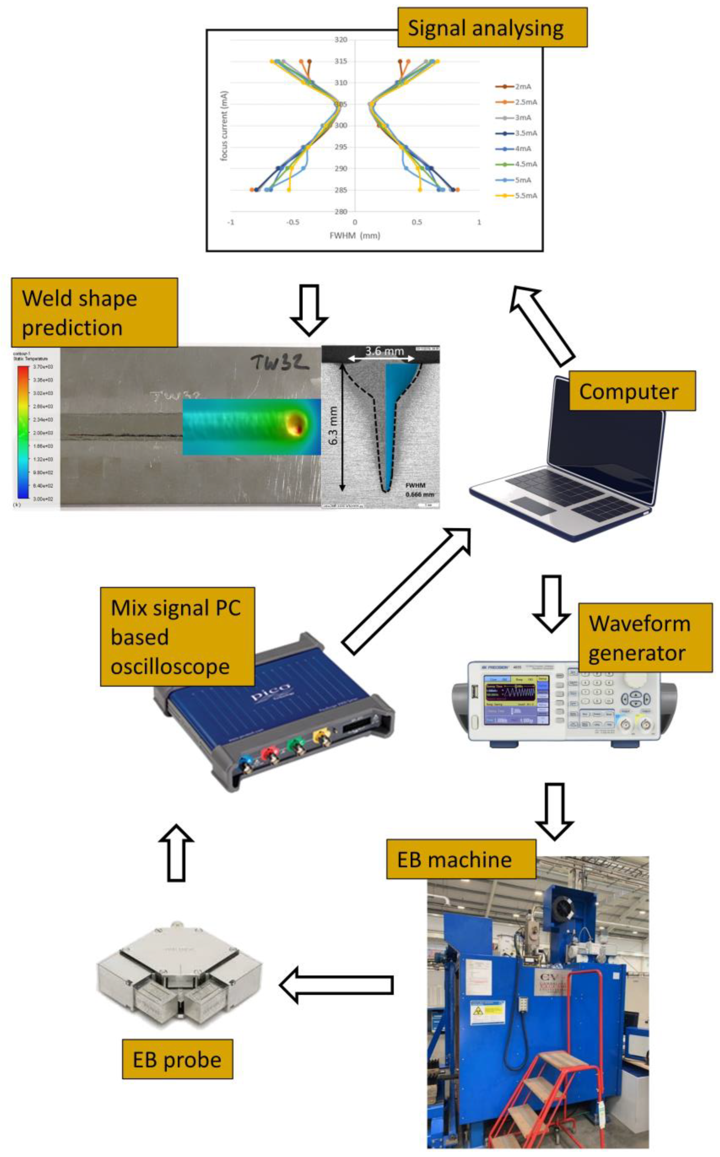
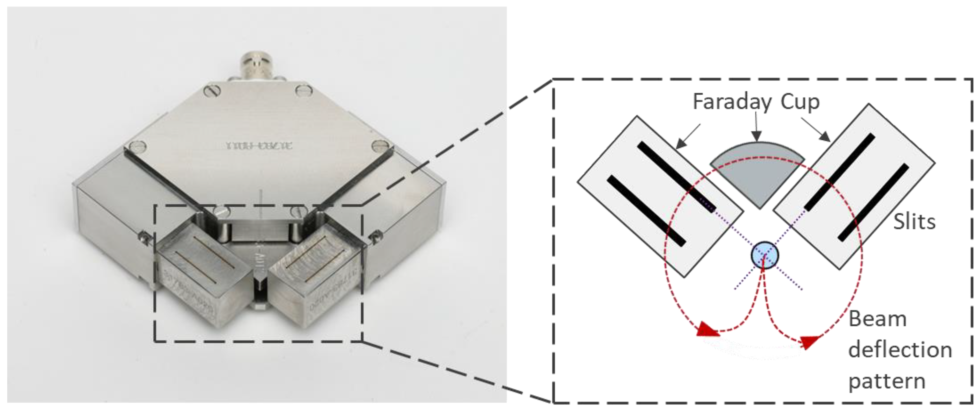
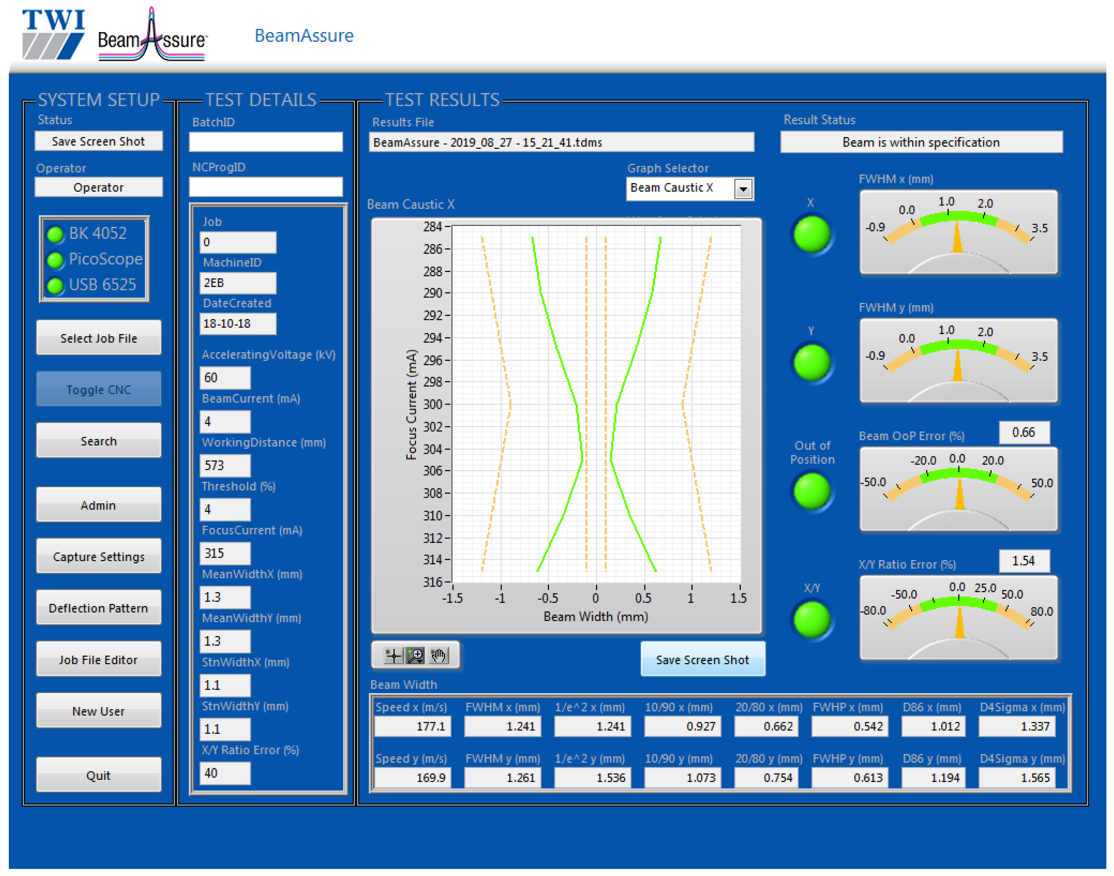
- Characterisation of electron beams: The electron beams are characterised using the method described in [2], allowing the beam radius in both the welding and cross-sectional directions to be identified. As a result, the beam characteristics can be easily incorporated into the CFD model as inputs, following a standard protocol.
- Simulation of a 2-s welding process: The CFD model has been adjusted to simulate a 2-s welding process, incorporating an efficient and easily understandable heat generation algorithm.
- Applications for neural network training: the CFD model is also suitable for training a neural network model. This allows for rapid and reliable penetration depth predictions in real industrial environments.
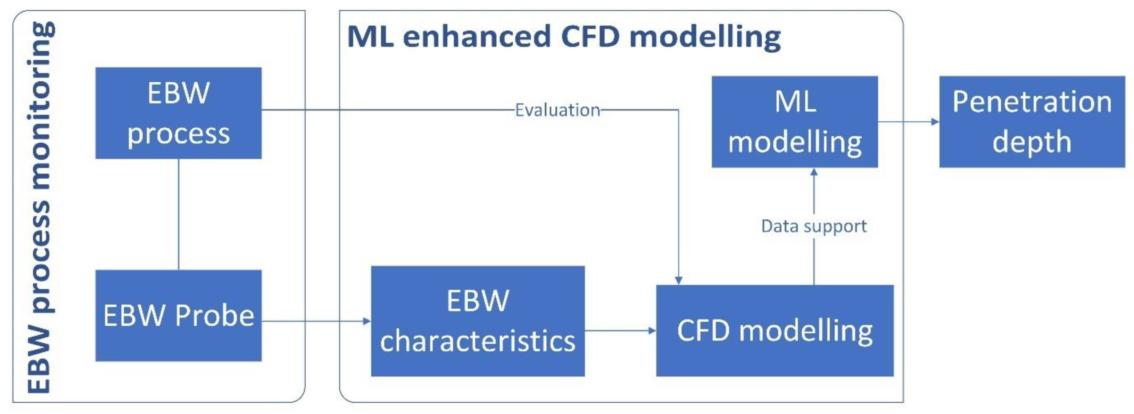
2. Methodology
3. EBW Process Monitoring
4. ML-Enhanced CFD Modelling
4.1. CFD Model Setup
- The molten pool was assumed to exhibit laminar flow, be incompressible, and behave as a Newtonian fluid. Based on previous simulation results, applying laminar flow and incompressible Newtonian fluid can successfully reproduce the EBW joining process [29]. The simulation complexity can be reduced without much impact on the simulation results.
- The electron beam power intensity was assumed to follow an ideal Gaussian distribution. This assumption may lead to discrepancies in CFD predictions, since the actual beam power may not strictly follow a Gaussian shape. This simplification, nonetheless, facilitates the determination of power distribution based on the beam radius.
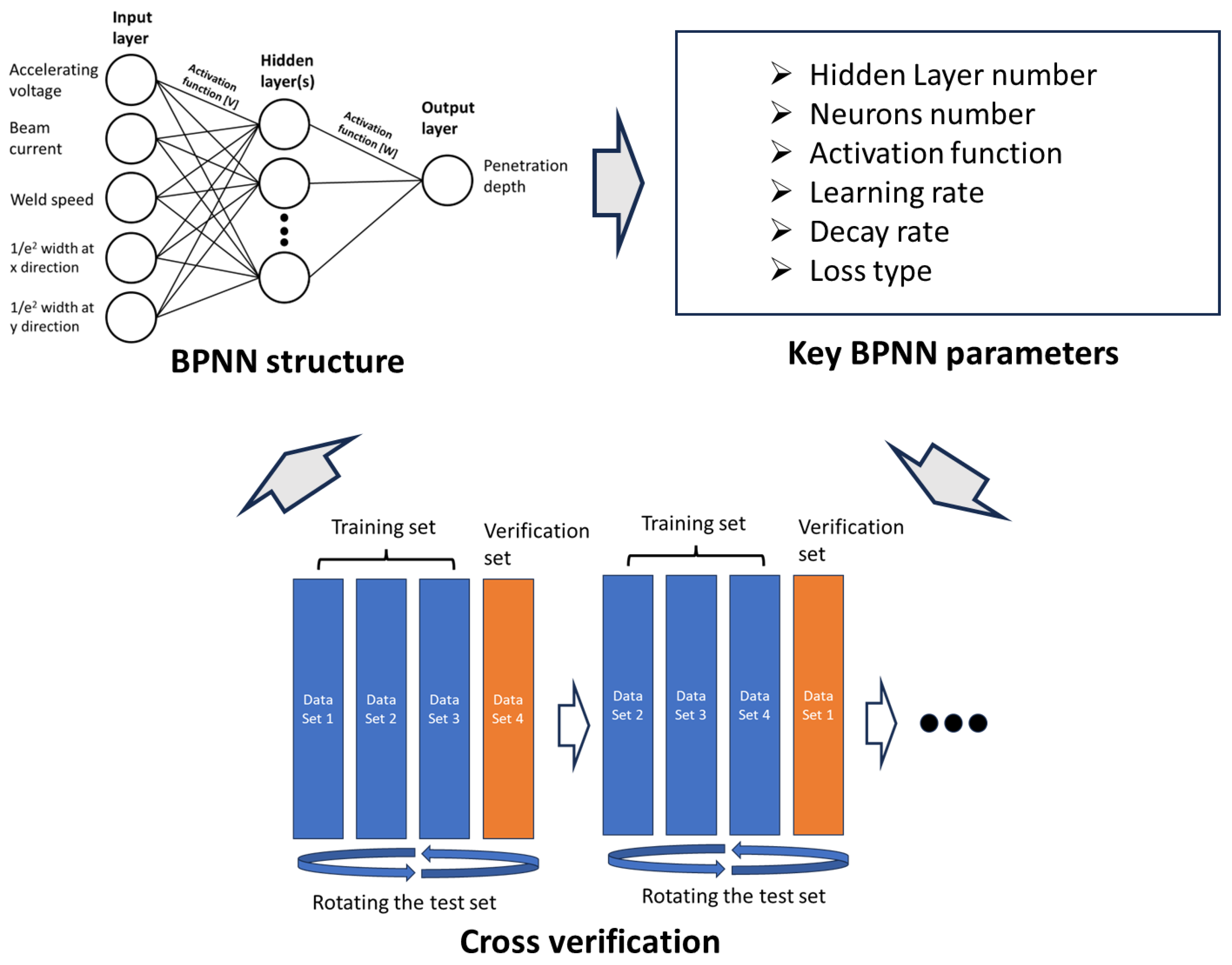
4.2. ML Model Setup
5. Results and Discussion
- (1)
- One hidden layer with 15 neurons.
- (2)
- Linear transfer function for the input layer and ‘softplus’ activation function for the hidden layer.
- (3)
- Type ‘Normal’ kernel initialiser for the input layer and the hidden layer.
- (4)
- ‘SGD’ optimiser: Initial learning rate is 0.001, decay steps 10,000, and decay rate 0.9.
- (5)
- Losses type: mean absolute percentage error.
- (6)
- 5000 iterations.
6. Conclusions
Author Contributions
Funding
Institutional Review Board Statement
Informed Consent Statement
Data Availability Statement
Conflicts of Interest
References
- Rai, R.; Burgardt, P.; Milewski, J.O.; Lienert, T.J.; Debroy, T. Heat transfer and fluid flow during electron beam welding of 21Cr–6Ni–9Mn steel and Ti–6Al–4V alloy. J. Phys. D Appl. Phys. 2009, 42, 025503. [Google Scholar] [CrossRef]
- Yin, Y.; Kennedy, A.; Mitchell, T.; Sieczkiewicz, N.; Jefimovs, V.; Tian, Y. Electron beam weld penetration depth prediction improved by beam characterisation. Int. J. Adv. Manuf. Technol. 2023, 125, 399–415. [Google Scholar] [CrossRef]
- Liu, C.-C.; He, J.-S. Numerical analysis of thermal fluid transport behavior during electron beam welding of 2219 aluminum alloy plate. Trans. Nonferrous Met. Soc. China 2017, 27, 1319–1326. [Google Scholar] [CrossRef]
- Tomashchuk, I.; Sallamand, P.; Jouvard, J.M.; Grevey, D. The simulation of morphology of dissimilar copper–steel electron beam welds using level set method. Comput. Mater. Sci. 2010, 48, 827–836. [Google Scholar] [CrossRef]
- Borrmann, S.; Kratzsch, C.; Halbauer, L.; Buchwalder, A.; Biermann, H.; Saenko, I.; Chattopadhyay, K.; Schwarze, R. Electron beam welding of CrMnNi-steels: CFD-modeling with temperature sensitive thermophysical properties. Int. J. Heat Mass Transf. 2019, 139, 442–455. [Google Scholar] [CrossRef]
- Liang, L.; Hu, R.; Wang, J.; Luo, M.; Huang, A.; Wu, B.; Pang, S. A CFD-FEM model of residual stress for electron beam welding including the weld imperfection effect. Metall. Mater. Trans. A 2019, 50, 2246–2258. [Google Scholar] [CrossRef]
- Chen, G.; Liu, J.; Shu, X.; Gu, H.; Zhang, B. Numerical simulation of keyhole morphology and molten pool flow behavior in aluminum alloy electron-beam welding. Int. J. Heat Mass Transf. J. 2019, 138, 879–888. [Google Scholar] [CrossRef]
- Yang, Z.; Fang, Y.; He, J. Numerical simulation of heat transfer and fluid flow during vacuum electron beam welding of 2219 aluminium girth joints. Vacuum 2020, 175, 109256. [Google Scholar] [CrossRef]
- Huang, B.; Chen, X.; Pang, S.; Hu, R. A three-dimensional model of coupling dynamics of keyhole and weld pool during electron beam welding. Int. J. Heat Mass Transf. 2017, 115, 159–173. [Google Scholar] [CrossRef]
- Luo, M.; Hu, R.; Liu, T.; Wu, B.; Pang, S. Optimization possibility of beam scanning for electron beam welding: Physics understanding and parameters selection criteria. Int. J. Heat Mass Transf. 2018, 127, 1313–1326. [Google Scholar] [CrossRef]
- Wang, J.; Hu, R.; Chen, X.; Pang, S. Modeling fluid dynamics of vapor plume in transient keyhole during vacuum electron beam welding. Vacuum 2018, 157, 277–290. [Google Scholar] [CrossRef]
- Wang, Y.; Fu, P.; Guan, Y.; Lu, Z.; Wei, Y. Research on modeling of heat source for electron beam welding fusion-solidification zone. Chin. J. Aeronaut. 2013, 26, 217–223. [Google Scholar] [CrossRef]
- Trushnikov, D.N.; Permyakov, G.L. Numerical simulation of electron beam welding with beam oscillations. In IOP Conference Series: Materials Science and Engineering; IOP Publishing: Bristol, UK, 2017. [Google Scholar]
- Yin, Y.; Jefimovs, V.; Mitchell, T.; Kennedy, A.; Williams, D.; Tian, Y. Numerical modelling of electron beam welding of pure niobium with beam oscillation: Towards Industry 4.0. In Proceedings of the 26th International Conference on Automation & Computing, Portsmouth, UK, 2–4 September 2021. [Google Scholar]
- Dey, V.; Pratihar, D.K.; Datta, G.L. Prediction of weld bead profile using neural networks. In Proceedings of the First International Conference on Emerging Trends in Engineering and Technology, Nagpur, India, 16–18 July 2008. [Google Scholar]
- Dey, V.; Pratihar, D.K.; Datta, G.L.; Jha, M.N.; Saha, T.K.; Bapat, A.V. Optimization and prediction of weldment profile in bead-on-plate welding of Al-1100 plates using electron beam. Int. J. Adv. Manuf. Technol. 2010, 48, 513–528. [Google Scholar] [CrossRef]
- Dey, V.; Pratihar, D.K.; Datta, G.L. Forward and reverse modeling of electron beam welding process using radial basis function neural networks. Int. J. Knowl.-Based Intellegent Eng. Syst. 2010, 14, 201–215. [Google Scholar] [CrossRef]
- Reddy, D.Y.; Pratihar, D.K. Neural network-based expert systems for predictions of temperature distributions in electron beam welding process. Int. J. Adv. Manuf. Technol. 2011, 55, 535–548. [Google Scholar] [CrossRef]
- Jha, M.N.; Pratihar, D.K.; Bapat, A.V.; Dey, V.; Ali, M.; Bagchi, A.C. Knowledge-based systems using neural networks for electron beam welding process of reactive material (Zircaloy-4). J. Intell. Manuf. 2014, 25, 1315–1333. [Google Scholar] [CrossRef]
- Shen, X.; Huang, W.; Xu, C.; Wang, X. Bi-directional prediction between weld penetration and processing parameters in electron beam welding using artificial neural. In Advances in Neural Networks–ISNN 2009, Proceedings of the 6th International Symposium on Neural Networks (ISNN 2009), Wuhan, China, 26–29 May 2009; Proceedings, Part III 6; Springer: Berlin/Heidelberg, Germany, 2009. [Google Scholar]
- Giedt, W.H.; Tallerico, L.N. Prediction of electron beam depth of penetration. Weld. J. 1988, 67, 299–305. [Google Scholar]
- Elmer, J.W.; Giedt, W.H.; Eagar, T.W. The transition from shallow to deep penetration during electron beam welding. Weld. J. 1990, 69, 167s–175s. [Google Scholar]
- Hemmer, H.; Grong, Ø. Prediction of penetration depths during electron beam welding. Sci. Technol. Weld. Join. 1999, 4, 219–225. [Google Scholar] [CrossRef]
- Xiao, J.; He, P.; Li, X.; Bénard, P.; Yang, T.; Chahine, R. Computational fluid dynamics model based artificial neural network prediction of flammable vapor clouds formed by liquid hydrogen releases. Int. J. Energy Res. 2022, 46, 11011–11026. [Google Scholar] [CrossRef]
- Kumar, M.K.H.; Vishweshwara, P.S.; Gnanasekaran, N. Evaluation of artificial neural network in data reduction for a natural convection conjugate heat transfer problem in an inverse approach: Experiments combined with CFD solutions. Sādhanā 2020, 45, 78. [Google Scholar] [CrossRef]
- Pandya, D.A.; Dennis, B.H.; Russell, R.D. A computational fluid dynamics based artificial neural network model to predict solid particle erosion. Wear 2017, 378, 198–210. [Google Scholar] [CrossRef]
- Wang, C.-N.; Yang, F.-C.; Nguyen, V.T.T.; Vo, N.T.M. CFD Analysis and optimum design for a centrifugal pump using an effectively artificial intelligent algorithm. Micromachines 2022, 13, 1208. [Google Scholar] [CrossRef] [PubMed]
- Ribton, C.; Ferhati, A.; Longfield, N.; Juffs, P. Production weld quality assurance through monitoring of beam characteristics. Електрoтехника Eлектрoника 2018, 53, 231–235. [Google Scholar]
- Borrmann, S.; Asad, A.; Halbauer, L.; Buchwalder, A.; Biermann, H. Numerical simulation of the particle displacement during electron beam welding of a dissimilar weld joint with TRIP-Matrix-Composite. Adv. Eng. Mater. 2019, 21, 1800741. [Google Scholar] [CrossRef]
- Brooks, R.F.; Quested, P.N. The surface tension of steels. J. Mater. Sci. 2005, 40, 2233–2238. [Google Scholar] [CrossRef]
- Gołdasz, A.; Gielzecki, J.; Malinowski, Z.; Rywotycki, M. Modelling liquid steel motion caused by electromagnetic stirring in continuous casting steel. Arch. Metall. Mater. 2014, 59, 487–492. [Google Scholar]
- Data, M.P. Ovako S275JR SB1412 Steel. Ovako. 2022. Available online: https://www.matweb.com/search/datasheet.aspx?matguid=c63e73e4a831418985cece9dd2607269&ckck=1 (accessed on 15 January 2023).
- Schultz, H. Electron Beam Welding; Woodhead Publishing: Sawston, UK, 1993. [Google Scholar]
- Huang, J. The Characterisation and Modelling of Porosity Formation in Electron Beam Welded Titanium Alloys. Ph.D. Thesis, University of Birmingham, Birmingham, UK, 2011. [Google Scholar]
- Burgardt, P.; Pierce, S.W.; Dvornak, M.J. Definition of Beam Diameter for Electron Beam Welding (No. LA-UR-16-21655); Los Alamos National Lab. (LANL): Los Alamos, NM, USA, 2016. [Google Scholar]
- Siddaiah, A.; Singh, B.K.; Mastanaiah, P. Prediction and optimization of weld bead geometry for electron beam welding of AISI 304 stainless steel. Int. J. Adv. Manuf. Technol. 2017, 89, 27–43. [Google Scholar] [CrossRef]


| Weld No. | Accelerating Voltage U (kV) | Beam Current I (mA) | Welding Speed S (mm/min) | Focusing Current and Relative Sharp Focus Current Ifr (mA) | Beam Radius (1/e2 Width σx) at x Direction (mm) | Beam Radius (1/e2 width σy) at y Direction (mm) | Measured Penetration Depth ± Standard Deviation (mm) |
|---|---|---|---|---|---|---|---|
| C1 | 40 | 45 | 650 | 280 (sharp-focus −6) | 0.571 | 0.704 | 4.24 ± 0.09 |
| C2 | 40 | 30 | 700 | 293 (sharp-focus +8) | 0.413 | 0.467 | 3.20 ± 0.05 |
| C3 | 50 | 40 | 700 | 316 (sharp-focus −4) | 0.377 | 0.455 | 6.36 ± 0.09 |
| C4 | 50 | 30 | 550 | 320 (sharp-focus −4) | 0.266 | 0.277 | 6.95 ± 0.19 |
| C5 | 60 | 45 | 500 | 340 (sharp-focus −8) | 0.520 | 0.517 | 10.66 ± 0.17 |
| C6 | 60 | 40 | 500 | 362 (sharp-focus +4) | 0.339 | 0.369 | 9.55 ± 0.26 |
| C7 | 60 | 40 | 700 | 354 (sharp-focus −4) | 0.330 | 0.346 | 9.36 ± 0.27 |
| C8 | 60 | 35 | 500 | 351 (sharp-focus −4) | 0.261 | 0.304 | 10.42 ± 0.38 |
| C9 | 60 | 30 | 650 | 360 (sharp-focus) | 0.208 | 0.277 | 8.10 ± 0.18 |
| C10 | 50 | 35 | 500 | 312 (sharp-focus −8) | 0.407 | 0.439 | 6.33 ± 0.20 |
| C11 | 50 | 25 | 550 | 329 (sharp-focus +4) | 0.251 | 0.319 | 5.56 ± 0.10 |
| C12 | 40 | 45 | 700 | 294 (sharp-focus +8) | 0.778 | 0.901 | 3.51 ± 0.10 |
| C13 | 40 | 40 | 650 | 278 (sharp-focus −8) | 0.501 | 0.622 | 4.31 ± 0.08 |
| C14 | 40 | 25 | 500 | 293 (sharp-focus +4) | 0.333 | 0.400 | 3.62 ± 0.11 |
| C15 | 40 | 35 | 600 | 285 (sharp-focus) | 0.435 | 0.540 | 4.55 ± 0.07 |
| C16 | 60 | 40 | 600 | 366 (sharp-focus +8) | 0.401 | 0.423 | 7.77 ± 0.16 |
| C17 | 60 | 25 | 500 | 353 (sharp-focus −8) | 0.312 | 0.266 | 8.04 ± 0.26 |
| C18 | 60 | 35 | 550 | 351 (sharp-focus −4) | 0.261 | 0.304 | 10.05 ± 0.35 |
| C19 | 40 | 45 | 650 | 286 (sharp-focus) | 0.631 | 0.794 | 4.37 ± 0.05 |
| C20 | 40 | 45 | 650 | 290 (sharp-focus +4) | 0.702 | 0.829 | 4.08 ± 0.04 |
| C21 | 40 | 35 | 650 | 277 (sharp-focus −8) | 0.450 | 0.571 | 3.75 ± 0.05 |
| C22 | 40 | 30 | 600 | 293 (sharp-focus +8) | 0.413 | 0.467 | 3.60 ± 0.07 |
| C23 | 50 | 30 | 700 | 316 (sharp-focus −8) | 0.336 | 0.350 | 5.45 ± 0.13 |
| C24 | 50 | 25 | 650 | 321 (sharp-focus −4) | 0.246 | 0.274 | 5.91 ± 0.44 |
| C25 | 50 | 35 | 600 | 320 (sharp-focus) | 0.304 | 0.366 | 7.01 ± 0.25 |
| C26 | 50 | 40 | 550 | 324 (sharp-focus +4) | 0.370 | 0.434 | 6.84 ± 0.31 |
| C27 | 50 | 45 | 500 | 326 (sharp-focus +8) | 0.495 | 0.605 | 7.26 ± 0.25 |
| C28 | 60 | 25 | 650 | 357 (sharp-focus −4) | 0.222 | 0.233 | 7.47 ± 0.23 |
| C29 | 60 | 30 | 550 | 364 (sharp-focus +4) | 0.250 | 0.322 | 7.49 ± 0.20 |
| C30 | 60 | 45 | 600 | 340 (sharp-focus −8) | 0.520 | 0.517 | 10.36 ± 0.23 |
| Physical Property | Value |
|---|---|
| Thermal conductivity | 52.11 W/(m × K) at 300 K |
| Density | 7840 kg/m³ |
| Latent heat of fusion | 288,482 J/kg |
| Solidus temperature | 1743 K |
| Liquidus temperature | 1788 K |
| Specific heat | 830 J/(kg × K) at 300 K |
| Surface tension | 1.8 N/m at 1850 K |
| Boiling point | 3135 K |
| Viscosity | 0.003 kg/(m × s) at 1800 K |
| Molecular | 55.845 kg/kmol |
| Model Parameters | Setting Value/Introduction |
|---|---|
| Mutiphase model | Homogenous model, Volume of Fluid (VOF) |
| Interface type | Sharp |
| Phases | Two phases (gas phase as the main phase) |
| Phase interaction | Continuum surface force with wall adhesion |
| Mushy zone parameter | 4,000,000 |
| Pressure–velocity coupling | SIMPLE |
| Solution controls | Default |
| No. | Depth 1 (mm) | Depth 2 (mm) | Depth 3 (mm) | Depth 4 (mm) | Depth 5 (mm) | Average Simulated Depth (mm) | Actual Depth (mm) |
|---|---|---|---|---|---|---|---|
| C1 | 4.75 | 4.5 | 4.75 | 4.5 | 4.75 | 4.65 | 4.24 |
| C2 | 4.25 | 3.75 | 4.25 | 3.75 | 4.25 | 4.05 | 3.2 |
| C3 | 6.25 | 6.75 | 6.25 | 6.5 | 6.25 | 6.4 | 6.36 |
| C4 | 6.5 | 7 | 6.75 | 7 | 6.75 | 6.8 | 6.95 |
| C5 | 8.25 | 8.5 | 8.25 | 8.25 | 8.25 | 8.3 | 10.66 |
| C6 | 9.75 | 10 | 9.75 | 10 | 9.75 | 9.85 | 9.55 |
| C7 | 9 | 10 | 9.75 | 9.75 | 9.5 | 9.6 | 9.36 |
| C8 | 10.25 | 10.25 | 10.25 | 10.25 | 10.25 | 10.25 | 10.42 |
| C9 | 8.75 | 8.75 | 9 | 8.75 | 9 | 8.85 | 8.1 |
| C10 | 5.5 | 6.5 | 6 | 6 | 5.5 | 5.9 | 6.33 |
| C11 | 6 | 6.25 | 6 | 6 | 6 | 6.05 | 5.56 |
| C12 | 3 | 3.5 | 3 | 3 | 3 | 3.1 | 3.51 |
| C13 | 4.25 | 4.75 | 4.75 | 4.75 | 4.5 | 4.6 | 4.31 |
| C14 | 4.25 | 4.25 | 5 | 4.25 | 4.75 | 4.5 | 3.62 |
| C15 | 4.5 | 4.5 | 4.75 | 5 | 4.75 | 4.7 | 4.55 |
| C16 | 7.75 | 8.25 | 8 | 8.25 | 8 | 8.05 | 7.77 |
| C17 | 6.5 | 7.25 | 7.25 | 7.25 | 7 | 7.05 | 8.04 |
| C18 | 9 | 9.25 | 9.25 | 9.25 | 9 | 9.15 | 10.05 |
| C19 | 3.75 | 4.5 | 4.25 | 4.5 | 4.25 | 4.25 | 4.37 |
| C20 | 3.75 | 3.75 | 3.75 | 3.75 | 3.75 | 3.75 | 4.08 |
| C21 | 4.25 | 4.25 | 4.25 | 4.25 | 4.25 | 4.25 | 3.75 |
| C22 | 3.75 | 4 | 3.75 | 3.75 | 3.75 | 3.8 | 3.6 |
| C23 | 5.5 | 5.75 | 5.25 | 5.75 | 5.5 | 5.55 | 5.45 |
| C24 | 5.5 | 6 | 5.75 | 5.75 | 5.5 | 5.7 | 5.91 |
| C25 | 7 | 7 | 7.25 | 7.25 | 7 | 7.1 | 7.01 |
| C26 | 6.75 | 7.5 | 7.5 | 7.5 | 7 | 7.25 | 6.84 |
| C27 | 6.25 | 6.5 | 6.5 | 6.5 | 6.25 | 6.4 | 7.26 |
| C28 | 7.5 | 8 | 7.75 | 7.75 | 7.75 | 7.75 | 7.47 |
| C29 | 7.5 | 8.5 | 7.5 | 8 | 7.5 | 7.8 | 7.49 |
| C30 | 8 | 8.75 | 8 | 8 | 8 | 8.15 | 10.36 |
| Accelerating Voltage (kV) | Beam Current I (mA) | Welding Speed S (mm/min) | Focal Position | Deviation of CFD Prediction | |
|---|---|---|---|---|---|
| C2 | 40 | 30 | 700 | Over-focus (+8 mA) | +26.56% |
| C5 | 60 | 45 | 500 | Under-focus (−8 mA) | −22.14% |
| C14 | 40 | 25 | 500 | Over-focus (sharp-focus +4) | +24.31% |
| C30 | 60 | 45 | 600 | Under-focus (−8 mA) | −21.33% |
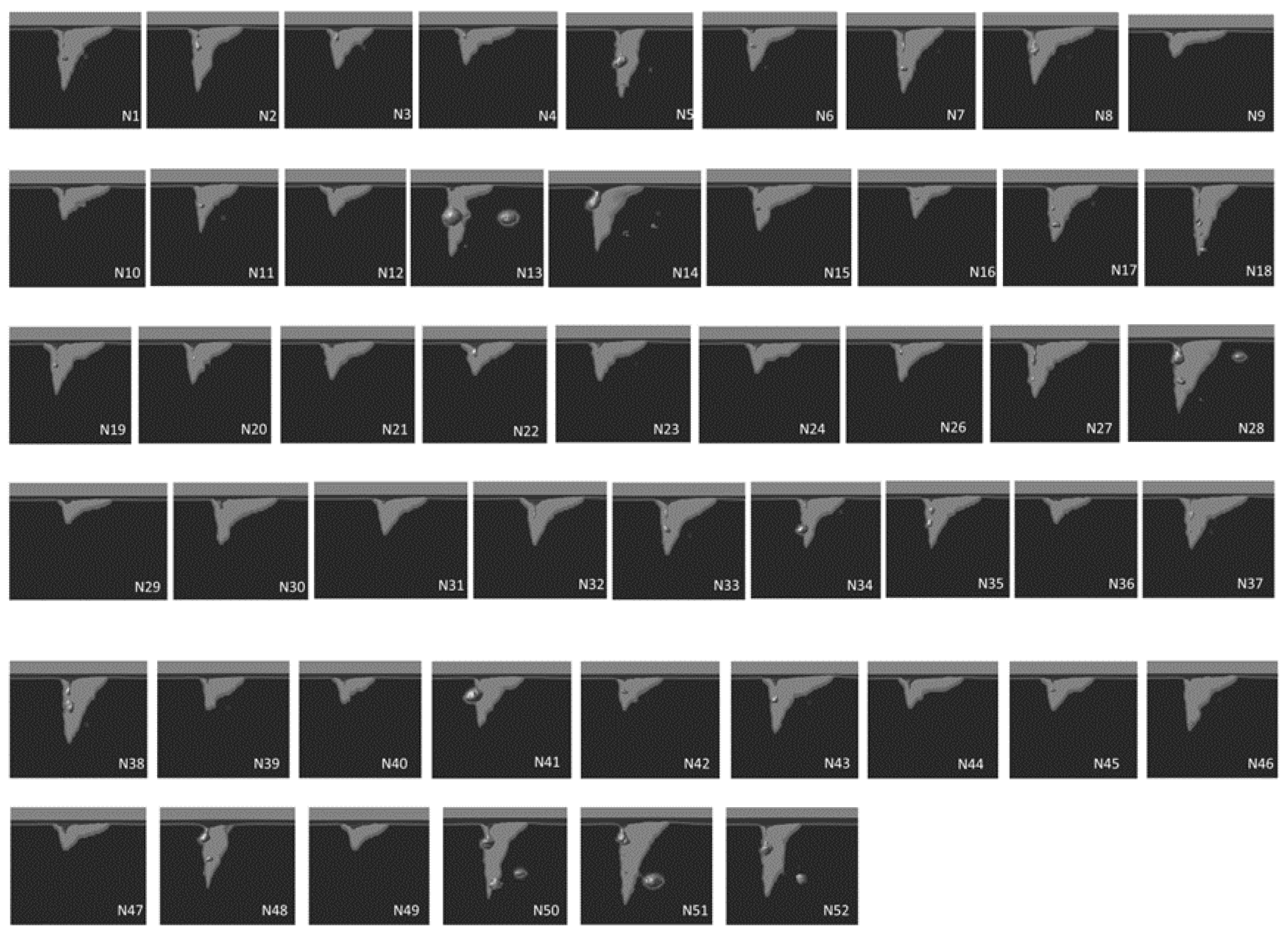
| No. | Accelerating Voltage U (kV) | Beam Current I (mA) | Welding Speed S (mm/min) | Beam Radius (1/e2 Width σx) at x Direction (mm) | Beam Radius (1/e2 Width σy) at y Direction (mm) | Depth at 1.2 s (mm) | Depth at 1.4 s (mm) | Depth at 1.6 s (mm) | Depth at 1.8 s (mm) | Depth at 2 s (mm) | Average Depth (mm) |
|---|---|---|---|---|---|---|---|---|---|---|---|
| N1 | 50 | 40 | 600 | 0.25 | 0.55 | 7.25 | 7.5 | 7.25 | 7.25 | 7.25 | 7.3 |
| N2 | 40 | 45 | 550 | 0.35 | 0.35 | 6.75 | 7.5 | 7.5 | 7.5 | 7 | 7.25 |
| N3 | 60 | 30 | 550 | 0.75 | 0.25 | 4.75 | 5.5 | 5.25 | 5.5 | 4.75 | 5.15 |
| N4 | 60 | 25 | 700 | 0.65 | 0.45 | 3.75 | 3.75 | 4.25 | 4 | 3.75 | 3.9 |
| N5 | 60 | 35 | 500 | 0.35 | 0.25 | 8 | 8.25 | 8.25 | 8.25 | 8 | 8.15 |
| N6 | 50 | 25 | 600 | 0.45 | 0.35 | 4.75 | 4.75 | 5 | 5 | 4.75 | 4.85 |
| N7 | 60 | 40 | 500 | 0.55 | 0.35 | 7.5 | 7.75 | 7.5 | 7.75 | 7.5 | 7.6 |
| N8 | 60 | 40 | 700 | 0.45 | 0.65 | 6.5 | 7 | 6.75 | 6.75 | 6.5 | 6.7 |
| N9 | 40 | 30 | 700 | 0.35 | 0.75 | 3 | 3 | 3 | 3.5 | 3 | 3.1 |
| N10 | 40 | 35 | 550 | 0.45 | 0.55 | 3.75 | 4.5 | 3.75 | 4.25 | 3.75 | 4 |
| N11 | 40 | 25 | 500 | 0.25 | 0.25 | 5.25 | 5.5 | 5.5 | 5.5 | 5.5 | 5.45 |
| N12 | 50 | 30 | 500 | 0.65 | 0.55 | 3.5 | 3.75 | 3.75 | 3.75 | 3.75 | 3.7 |
| N13 | 40 | 45 | 700 | 0.25 | 0.25 | 8 | 8.25 | 8.25 | 8.5 | 8.25 | 8.25 |
| N14 | 50 | 30 | 700 | 0.25 | 0.25 | 7.5 | 7.5 | 7.5 | 7.5 | 7.5 | 7.5 |
| N15 | 50 | 35 | 700 | 0.75 | 0.35 | 5 | 6 | 5.25 | 6 | 5.25 | 5.5 |
| N16 | 40 | 25 | 600 | 0.35 | 0.45 | 3.75 | 4.25 | 3.75 | 3.75 | 3.75 | 3.85 |
| N17 | 60 | 30 | 550 | 0.45 | 0.25 | 6 | 6.75 | 6.5 | 6.75 | 6.25 | 6.45 |
| N18 | 60 | 35 | 550 | 0.25 | 0.45 | 8.25 | 8.5 | 8.25 | 8.5 | 8.25 | 8.35 |
| N19 | 60 | 30 | 500 | 0.35 | 0.55 | 6 | 6 | 6 | 6 | 6 | 6 |
| N20 | 50 | 30 | 550 | 0.55 | 0.25 | 4.75 | 5 | 5 | 5 | 4.75 | 4.9 |
| N21 | 50 | 25 | 500 | 0.65 | 0.25 | 3.75 | 4.25 | 4.25 | 4.25 | 3.75 | 4.05 |
| N22 | 40 | 40 | 500 | 0.75 | 0.45 | 3.75 | 4.25 | 4.25 | 4.25 | 3.75 | 4.05 |
| N23 | 40 | 35 | 600 | 0.55 | 0.25 | 3.75 | 4.5 | 4.5 | 4.5 | 4.5 | 4.35 |
| N24 | 40 | 30 | 500 | 0.55 | 0.65 | 3 | 3.5 | 3 | 3.5 | 3 | 3.2 |
| N25 | 50 | 25 | 550 | 0.35 | 0.65 | 4.25 | 4.75 | 4.5 | 4.75 | 4.5 | 4.55 |
| N26 | 60 | 45 | 650 | 0.75 | 0.55 | 6.5 | 6.75 | 6.5 | 6.5 | 6.5 | 6.55 |
| N27 | 40 | 40 | 550 | 0.65 | 0.75 | 3.5 | 3.75 | 3.75 | 3.75 | 3.75 | 3.7 |
| N28 | 50 | 40 | 650 | 0.35 | 0.25 | 8.25 | 8.25 | 8.5 | 8.5 | 8.25 | 8.35 |
| N29 | 40 | 25 | 700 | 0.55 | 0.55 | 3 | 2.75 | 3 | 3 | 3 | 2.95 |
| N30 | 60 | 25 | 550 | 0.25 | 0.75 | 4.5 | 5.25 | 5 | 5.25 | 4.75 | 4.95 |
| N31 | 40 | 30 | 500 | 0.45 | 0.45 | 4.25 | 4.25 | 4.25 | 4.25 | 4.25 | 4.25 |
| N32 | 50 | 45 | 500 | 0.45 | 0.75 | 5.5 | 6 | 5.75 | 5.75 | 5.75 | 5.75 |
| N33 | 50 | 45 | 550 | 0.55 | 0.45 | 6.5 | 7 | 6.5 | 7 | 6.5 | 6.7 |
| N34 | 60 | 25 | 500 | 0.25 | 0.35 | 5.75 | 6.75 | 6 | 6 | 5.75 | 6.05 |
| N35 | 60 | 30 | 600 | 0.25 | 0.65 | 6 | 6 | 6 | 6 | 6 | 6 |
| N36 | 40 | 30 | 600 | 0.75 | 0.75 | 2.75 | 3 | 3 | 3 | 3 | 2.95 |
| N37 | 50 | 35 | 500 | 0.25 | 0.75 | 5.25 | 5.5 | 5.5 | 5.75 | 5.5 | 5.5 |
| N38 | 60 | 45 | 600 | 0.65 | 0.25 | 7.75 | 8.5 | 8.25 | 8.25 | 8 | 8.15 |
| N39 | 40 | 25 | 550 | 0.25 | 0.55 | 3.75 | 4.25 | 3.75 | 3.75 | 3.75 | 3.85 |
| N40 | 40 | 25 | 500 | 0.75 | 0.25 | 3 | 3 | 3 | 3 | 3 | 3 |
| N41 | 40 | 30 | 650 | 0.25 | 0.35 | 5.25 | 5.75 | 5.5 | 5.75 | 5.5 | 5.55 |
| N42 | 40 | 25 | 650 | 0.45 | 0.25 | 3.75 | 3.75 | 3.75 | 3.75 | 3.75 | 3.75 |
| N43 | 40 | 45 | 500 | 0.25 | 0.65 | 5.5 | 6.5 | 6.25 | 6.25 | 6 | 6.1 |
| N44 | 60 | 25 | 650 | 0.55 | 0.75 | 3.5 | 3.75 | 3.5 | 3.5 | 3.5 | 3.55 |
| N45 | 40 | 30 | 550 | 0.65 | 0.35 | 3.75 | 3.75 | 3.75 | 3.75 | 3.75 | 3.75 |
| N46 | 50 | 30 | 650 | 0.25 | 0.45 | 6.25 | 5.75 | 6.25 | 6.25 | 6.25 | 6.15 |
| N47 | 40 | 35 | 650 | 0.65 | 0.65 | 3 | 3.75 | 3.5 | 3.5 | 3.5 | 3.45 |
| N48 | 40 | 40 | 550 | 0.25 | 0.25 | 6.5 | 7.5 | 7 | 7.25 | 6.75 | 7 |
| N49 | 50 | 25 | 550 | 0.75 | 0.65 | 3 | 3 | 3 | 3 | 3 | 3 |
| N50 | 50 | 45 | 500 | 0.25 | 0.25 | 10 | 10.5 | 10.5 | 10.5 | 10.5 | 10.4 |
| N51 | 50 | 40 | 550 | 0.25 | 0.35 | 8 | 9.5 | 9.25 | 9.5 | 8.75 | 9 |
| N52 | 50 | 40 | 600 | 0.35 | 0.25 | 8.5 | 8.5 | 8.5 | 8.5 | 8.5 | 8.5 |
Disclaimer/Publisher’s Note: The statements, opinions and data contained in all publications are solely those of the individual author(s) and contributor(s) and not of MDPI and/or the editor(s). MDPI and/or the editor(s) disclaim responsibility for any injury to people or property resulting from any ideas, methods, instructions or products referred to in the content. |
© 2023 by the authors. Licensee MDPI, Basel, Switzerland. This article is an open access article distributed under the terms and conditions of the Creative Commons Attribution (CC BY) license (https://creativecommons.org/licenses/by/4.0/).
Share and Cite
Yin, Y.; Tian, Y.; Ding, J.; Mitchell, T.; Qin, J. Prediction of Electron Beam Welding Penetration Depth Using Machine Learning-Enhanced Computational Fluid Dynamics Modelling. Sensors 2023, 23, 8687. https://doi.org/10.3390/s23218687
Yin Y, Tian Y, Ding J, Mitchell T, Qin J. Prediction of Electron Beam Welding Penetration Depth Using Machine Learning-Enhanced Computational Fluid Dynamics Modelling. Sensors. 2023; 23(21):8687. https://doi.org/10.3390/s23218687
Chicago/Turabian StyleYin, Yi, Yingtao Tian, Jialuo Ding, Tim Mitchell, and Jian Qin. 2023. "Prediction of Electron Beam Welding Penetration Depth Using Machine Learning-Enhanced Computational Fluid Dynamics Modelling" Sensors 23, no. 21: 8687. https://doi.org/10.3390/s23218687
APA StyleYin, Y., Tian, Y., Ding, J., Mitchell, T., & Qin, J. (2023). Prediction of Electron Beam Welding Penetration Depth Using Machine Learning-Enhanced Computational Fluid Dynamics Modelling. Sensors, 23(21), 8687. https://doi.org/10.3390/s23218687