


3D Ultrasonic Brain Imaging with Deep Learning Based on Fully Convolutional Networks
 ,
, 
Abstract
1. Introduction
2. Methods
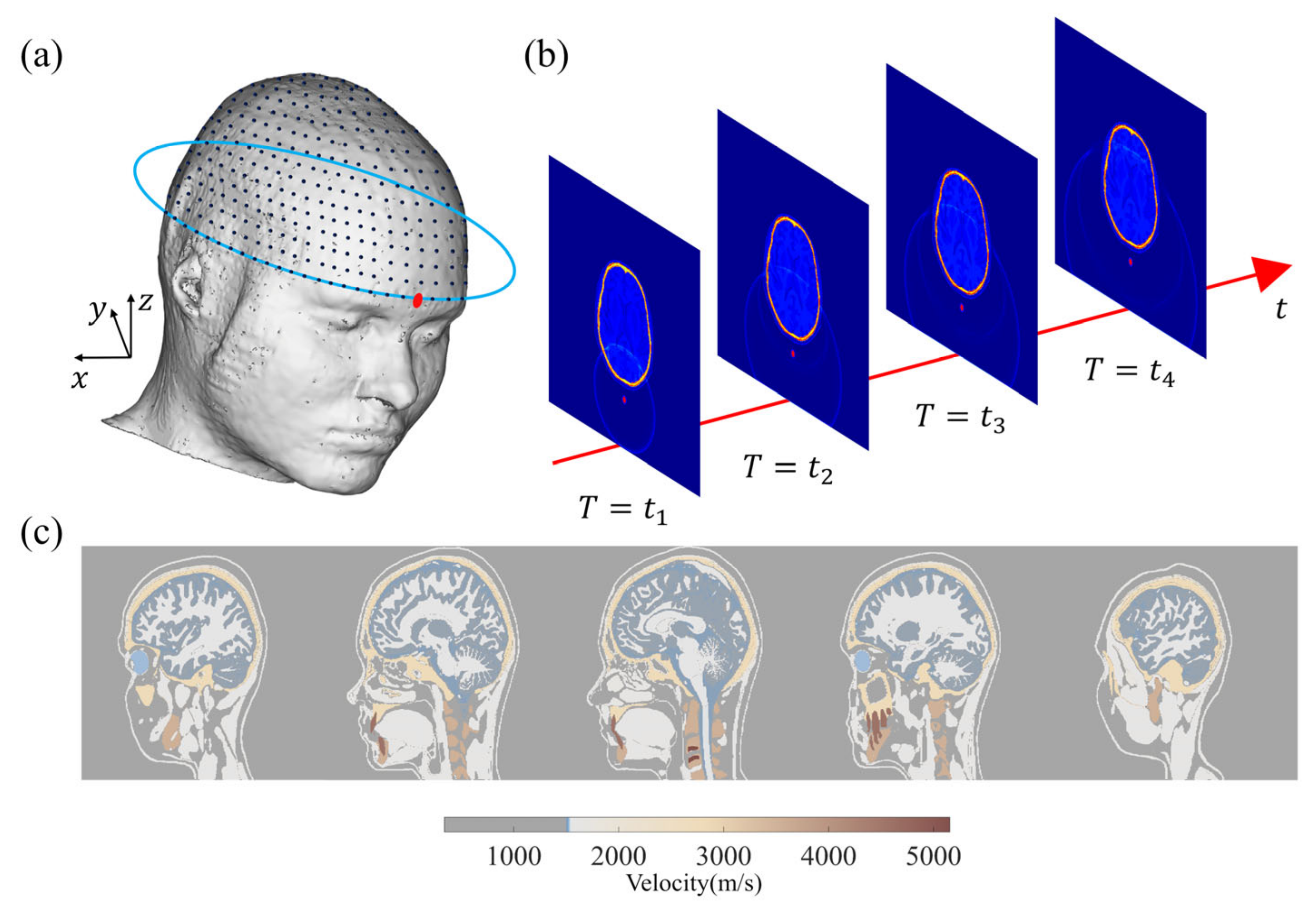
2.1. Three-Dimensional Wavefield Forward and Modeling
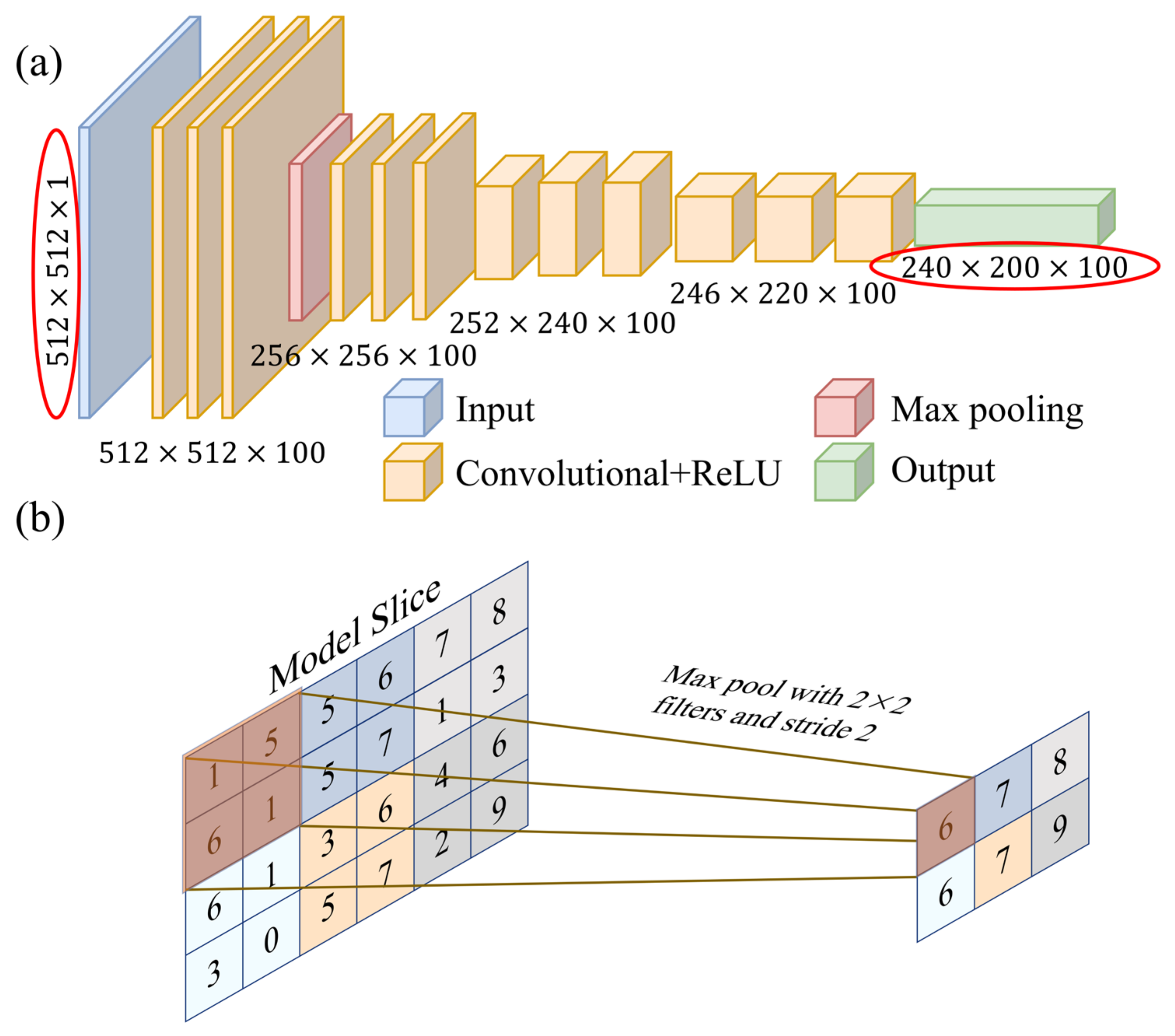
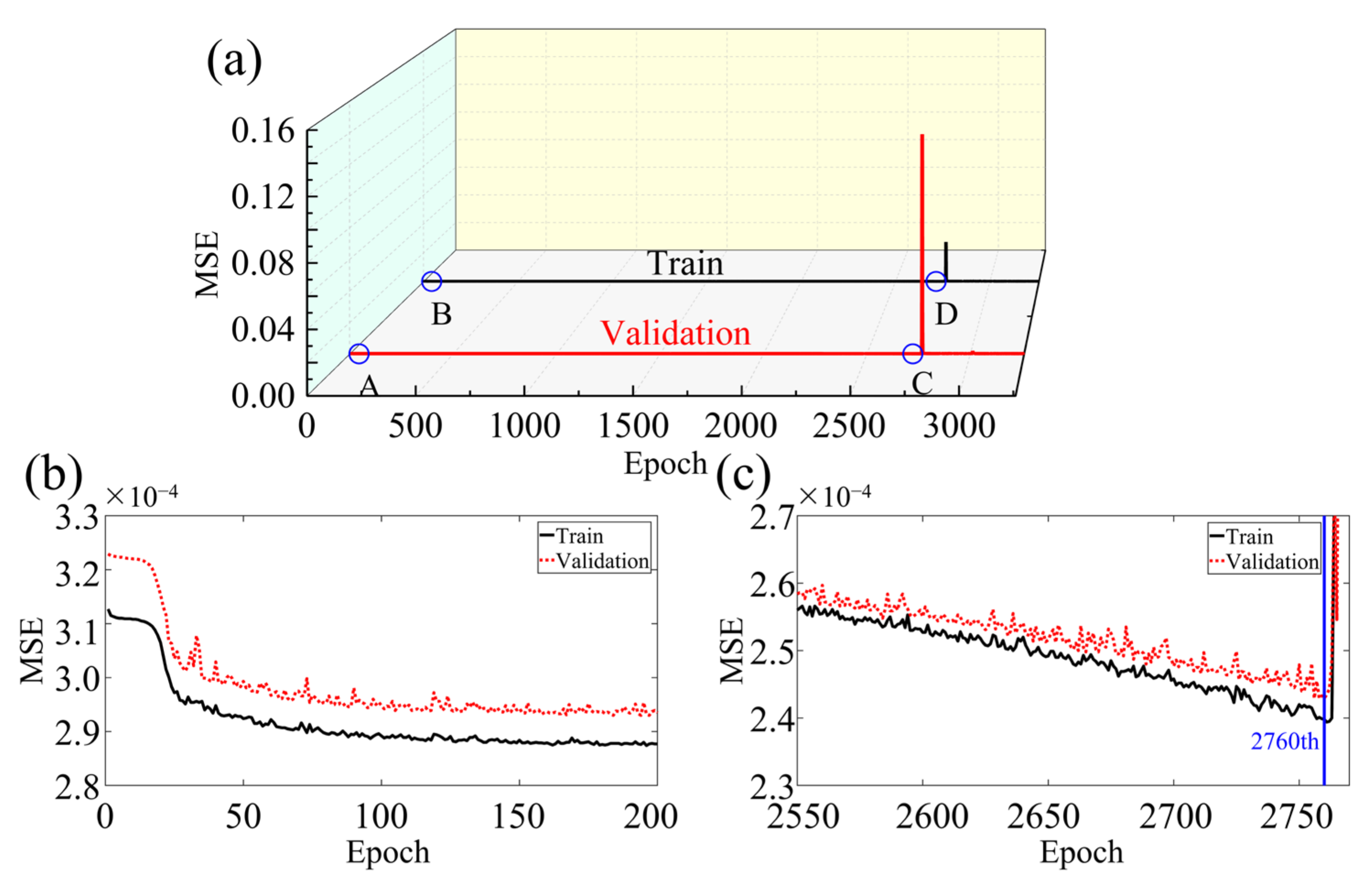
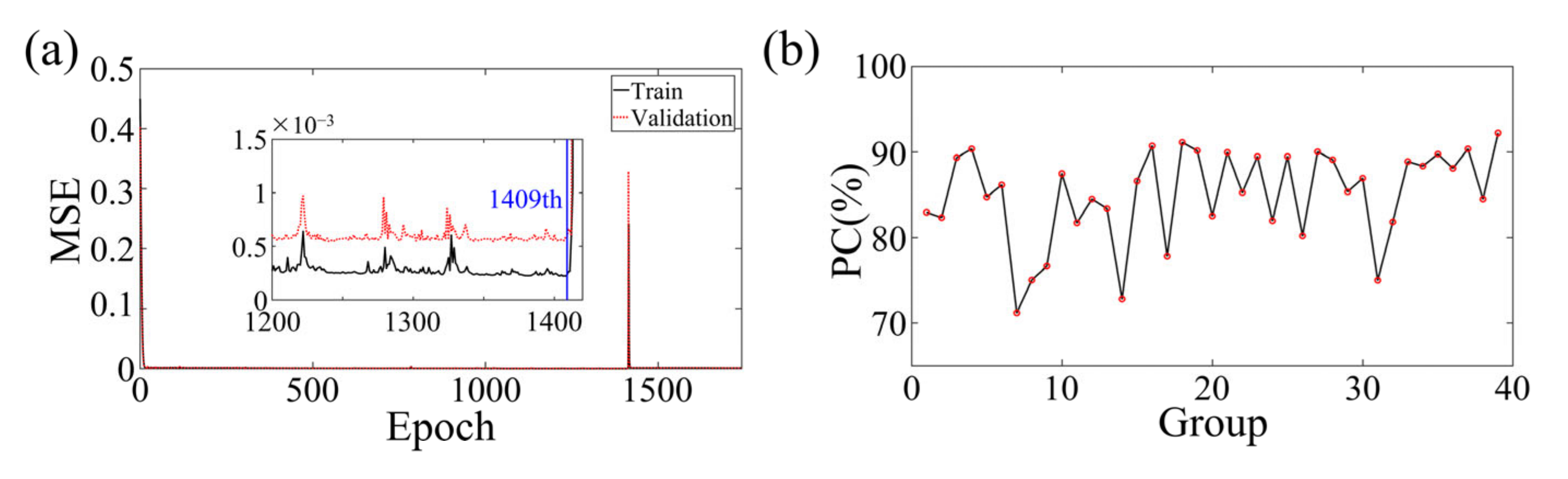
2.2. Two-Dimensional Fully Convolutional Network
2.3. Dataset Preprocessing and Reconstructed Image Evaluation
2.3.1. Dataset Preprocessing
2.3.2. Image Correlation Coefficient
3. Numerical Simulation
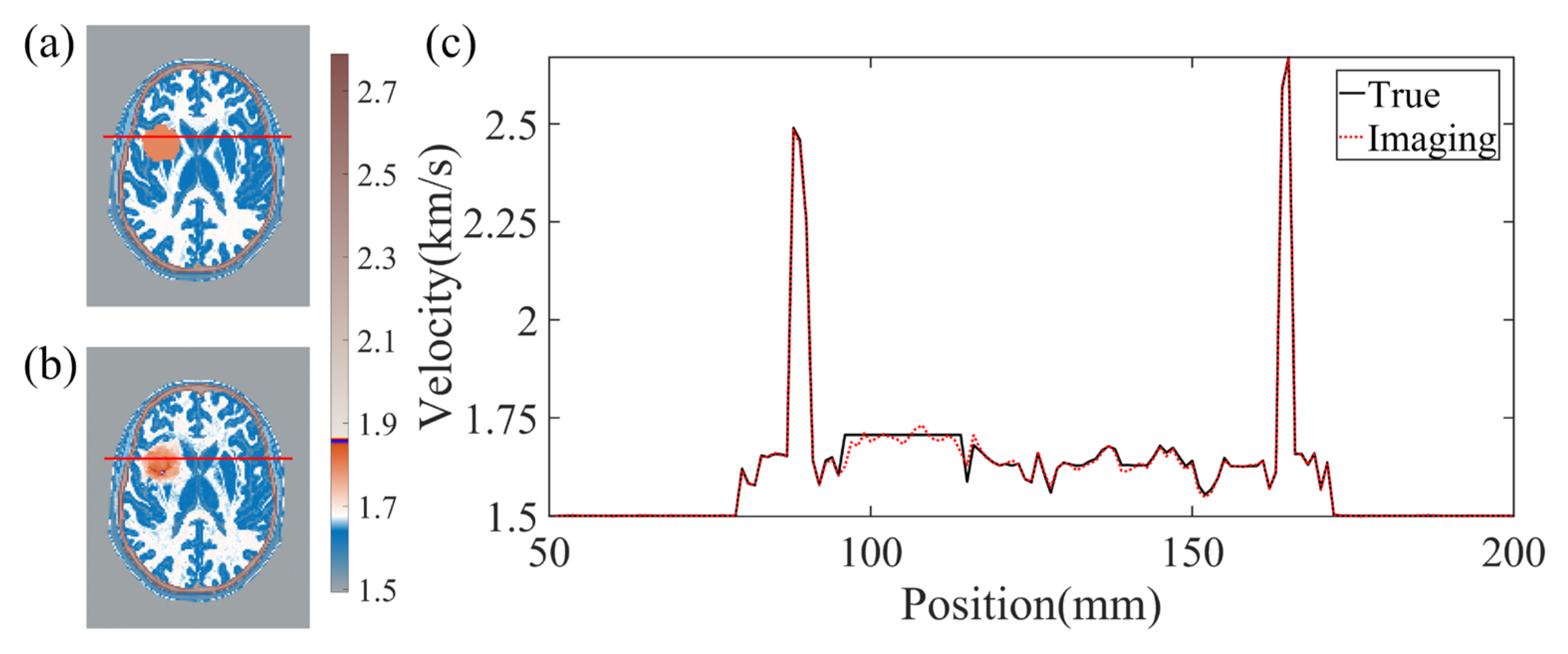
3.1. Two-Dimensional Horizontal Cross-Section Simulation Experiment
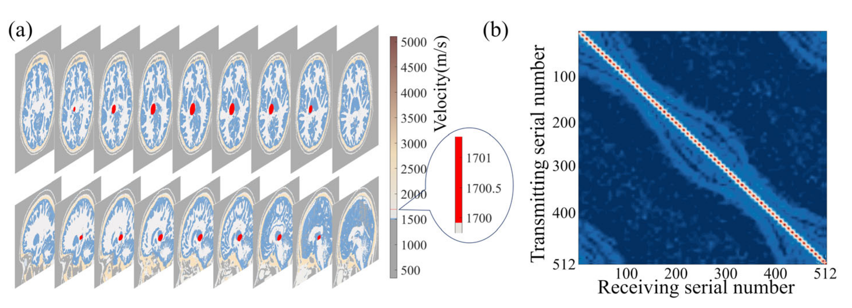
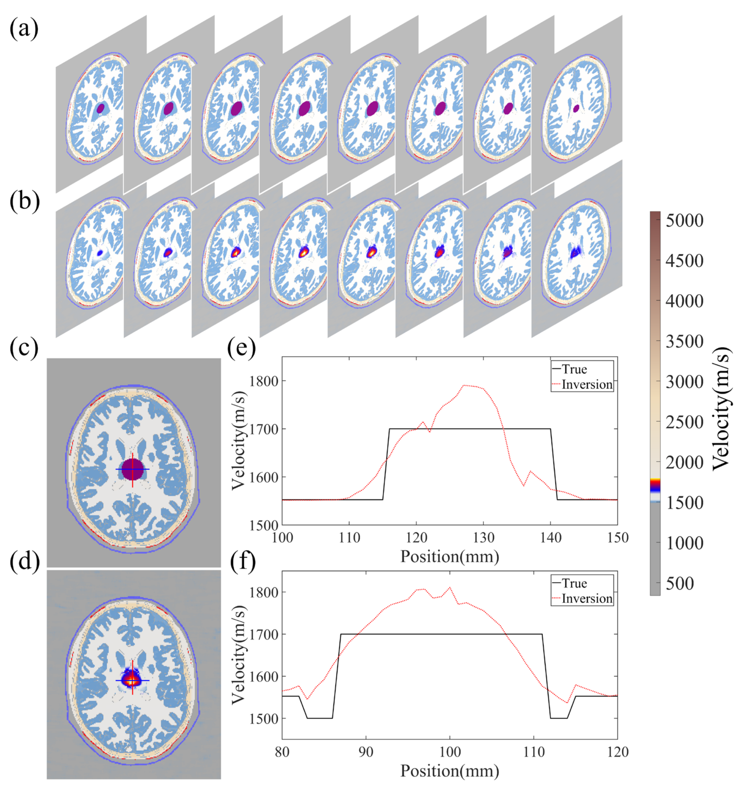
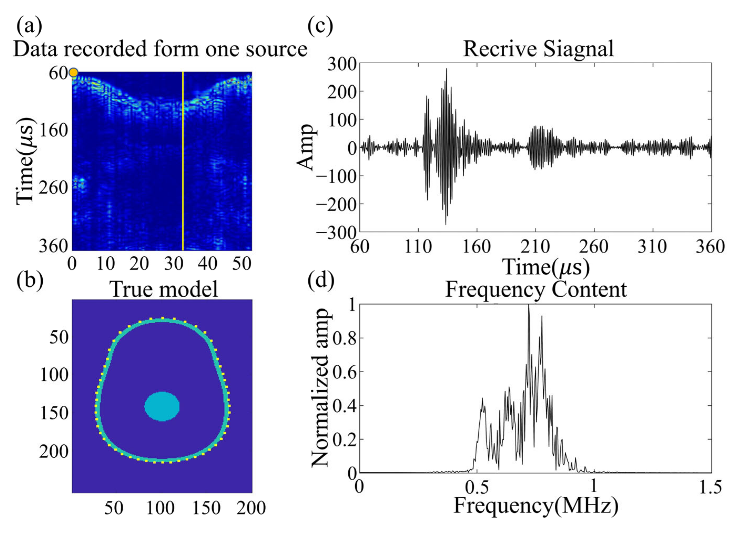
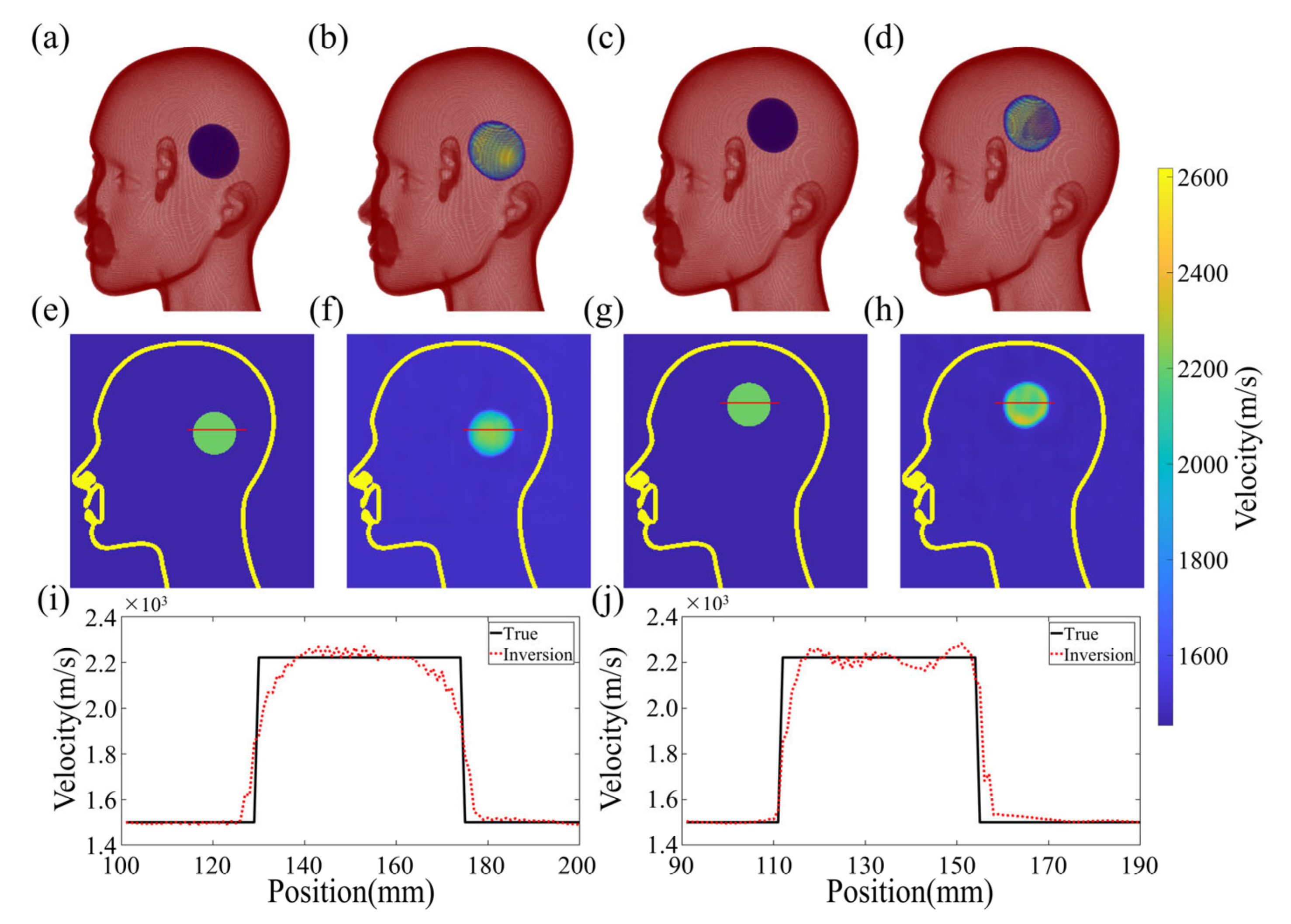
3.2. Three-Dimensional Brain Simulation Experiment
4. Laboratory Experimental Results
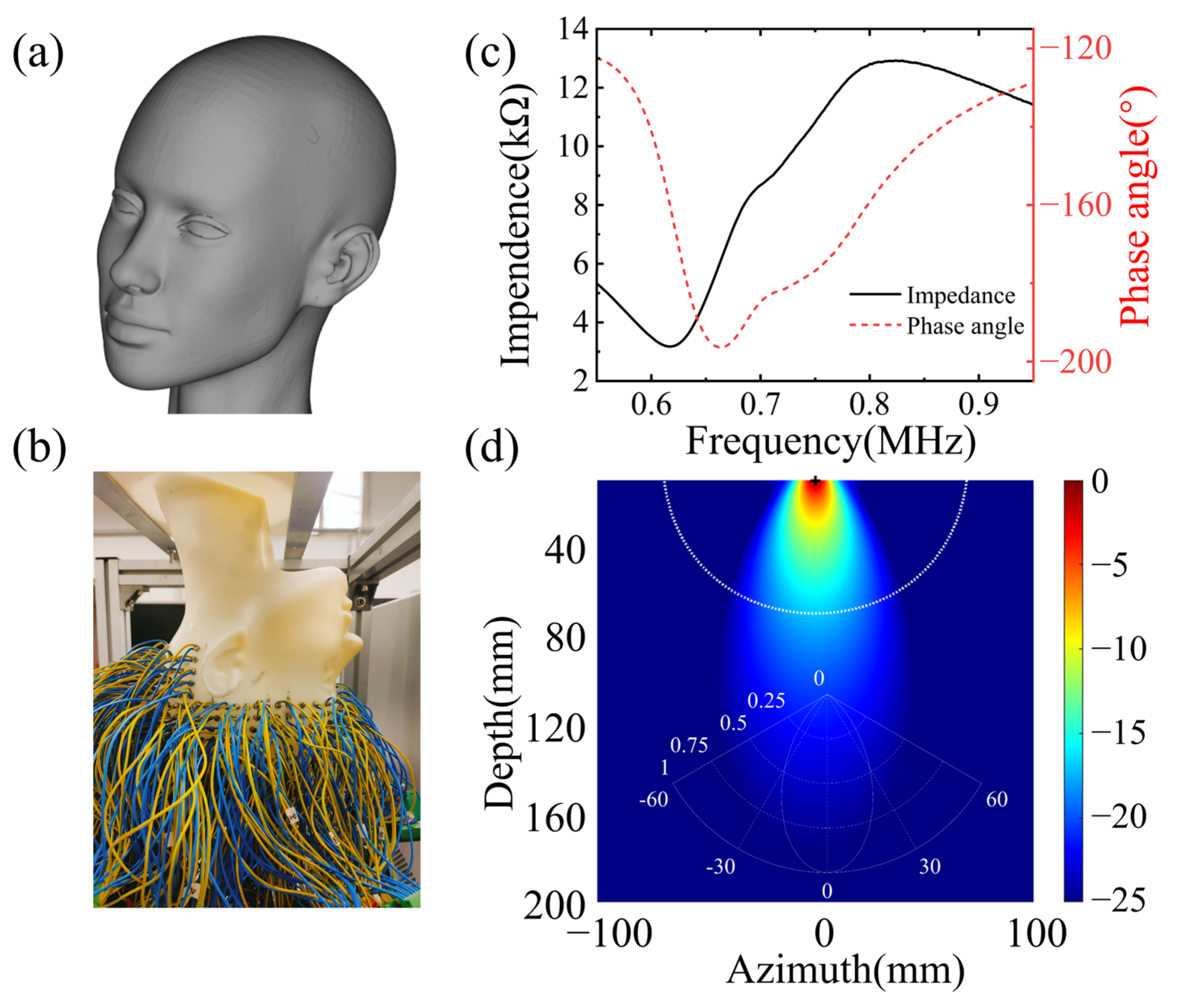
4.1. Experiment Preparation
4.2. Reconstruction Results
5. Discussion
5.1. Advantages and Achievements
5.2. Limitations and Solutions
6. Conclusions
Author Contributions
Funding
Institutional Review Board Statement
Informed Consent Statement
Data Availability Statement
Conflicts of Interest
References
- Edlow, B.L.; Mareyam, A.; Horn, A.; Polimeni, J.R.; Witzel, T.; Tisdall, M.D.; Augustinack, J.C.; Stockmann, J.P.; Diamond, B.R.; Stevens, A.; et al. 7 Tesla MRI of the ex vivo human brain at 100 micron resolution. Sci. Data 2019, 6, 244. [Google Scholar] [CrossRef]
- Yanagawa, M.; Hata, A.; Honda, O.; Kikuchi, N.; Miyata, T.; Uranishi, A.; Tsukagoshi, S.; Tomiyama, N. Subjective and objective comparisons of image quality between ultra-high-resolution CT and conventional area detector CT in phantoms and cadaveric human lungs. Eur. Radiol. 2018, 28, 5060–5068. [Google Scholar] [CrossRef] [PubMed]
- Menikou, G.; Dadakova, T.; Pavlina, M.; Bock, M.; Damianou, C. MRI compatible head phantom for ultrasound surgery. Ultrasonics 2015, 57, 144–152. [Google Scholar] [CrossRef]
- Monfrini, R.; Rossetto, G.; Scalona, E.; Galli, M.; Cimolin, V.; Lopomo, N.F. Technological Solutions for Human Movement Analysis in Obese Subjects: A Systematic Review. Sensors 2023, 23, 3175. [Google Scholar] [CrossRef] [PubMed]
- Kakkar, P.; Kakkar, T.; Patankar, T.; Saha, S. Current approaches and advances in the imaging of stroke. Dis. Models Mech. 2021, 14, dmm048785. [Google Scholar] [CrossRef] [PubMed]
- Goncalves, R.; Haueisen, J. Three-Dimensional Immersion Scanning Technique: A Scalable Low-Cost Solution for 3D Scanning Using Water-Based Fluid. Sensors 2023, 23, 3214. [Google Scholar] [CrossRef]
- Reyes-Santias, F.; Garcia-Garcia, C.; Aibar-Guzman, B.; Garcia-Campos, A.; Cordova-Arevalo, O.; Mendoza-Pintos, M.; Cinza-Sanjurjo, S.; Portela-Romero, M.; Mazon-Ramos, P.; Gonzalez-Juanatey, J.R. Cost Analysis of Magnetic Resonance Imaging and Computed Tomography in Cardiology: A Case Study of a University Hospital Complex in the Euro Region. Healthcare 2023, 11, 2084. [Google Scholar] [CrossRef]
- Wei, Y.; Yu, H.; Geng, J.S.; Wu, B.S.; Guo, Z.D.; He, L.Y.; Chen, Y.Y. Hospital efficiency and utilization of high-technology medical equipment: A panel data analysis. Health Policy Technol. 2018, 7, 65–72. [Google Scholar] [CrossRef]
- Riis, T.S.; Webb, T.D.; Kubanek, J. Acoustic properties across the human skull. Ultrasonics 2022, 119, 106591. [Google Scholar] [CrossRef] [PubMed]
- Park, C.Y.; Seo, H.; Lee, E.H.; Han, M.; Choi, H.; Park, K.S.; Yoon, S.Y.; Chang, S.H.; Park, J. Verification of Blood-Brain Barrier Disruption Based on the Clinical Validation Platform Using a Rat Model with Human Skull. Brain Sci. 2021, 11, 1429. [Google Scholar] [CrossRef]
- Manwar, R.; Kratkiewicz, K.; Avanaki, K. Investigation of the Effect of the Skull in Transcranial Photoacoustic Imaging: A Preliminary Ex Vivo Study. Sensors 2020, 20, 4189. [Google Scholar] [CrossRef] [PubMed]
- Wang, X.D.; Lin, W.J.; Su, C.; Wang, X.M. Influence of mode conversions in the skull on transcranial focused ultrasound and temperature fields utilizing the wave field separation method: A numerical study. Chin. Phys. B 2018, 27, 024302. [Google Scholar] [CrossRef]
- Jing, B.W.; Arvanitis, C.D.; Lindsey, B.D. Effect of incidence angle and wave mode conversion on transcranial ultrafast Doppler imaging. In Proceedings of the 2020 IEEE International Ultrasonics Symposium (IUS), Las Vegas, NV, USA, 7–11 September 2020. [Google Scholar]
- Paladini, D.; Vassallo, N.; Sglavo, G.; Pastore, G.; Lapadula, C.; Nappi, C. Normal and abnormal development of the fetal anterior fontanelle: A three-dimensional ultrasound study. Ultrasound Obstetr. Gynecol. 2008, 32, 755–761. [Google Scholar] [CrossRef]
- Raghuram, H.; Keunen, B.; Soucier, N.; Looi, T.; Pichardo, S.; Waspe, A.C.; Drake, J.M. A robotic magnetic resonance-guided high-intensity focused ultrasound platform for neonatal neurosurgery: Assessment of targeting accuracy and precision in a brain phantom. Med. Phys. 2022, 49, 2120–2135. [Google Scholar] [CrossRef]
- Yoshii, Y.; Villarraga, H.R.; Henderson, J.; Zhao, C.; An, K.N.; Amadio, P.C. Speckle Tracking Ultrasound for Assessment of the Relative Motion of Flexor Tendon and Subsynovial Connective Tissue in the Human Carpal Tunnel. Ultrasound Med. Biol. 2009, 35, 1973–1981. [Google Scholar] [CrossRef]
- Zhang, H.F.; Maslov, K.; Stoica, G.; Wang, L.H.V. Functional photoacoustic microscopy for high-resolution and noninvasive in vivo imaging. Nat. Biotechnol. 2006, 24, 848–851. [Google Scholar] [CrossRef] [PubMed]
- Kratkiewicz, K.; Manwar, R.; Zafar, M.; Ranjbaran, S.M.; Mozaffarzadeh, M.; de Jong, N.; Ji, K.L.; Avanaki, K. Development of a Stationary 3D Photoacoustic Imaging System Using Sparse Single-Element Transducers: Phantom Study. Appl. Sci. 2019, 9, 4505. [Google Scholar] [CrossRef]
- Barbosa, R.C.S.; Mendes, P.M. A Comprehensive Review on Photoacoustic-Based Devices for Biomedical Applications. Sensors 2022, 22, 9541. [Google Scholar] [CrossRef] [PubMed]
- Lutzweiler, C.; Razansky, D. Optoacoustic Imaging and Tomography: Reconstruction Approaches and Outstanding Challenges in Image Performance and Quantification. Sensors 2013, 13, 7345–7384. [Google Scholar] [CrossRef] [PubMed]
- Li, L.; Zhu, L.R.; Ma, C.; Lin, L.; Yao, J.J.; Wang, L.D.; Maslov, K.; Zhang, R.Y.; Chen, W.Y.; Shi, J.H.; et al. Single-impulse panoramic photoacoustic computed tomography of small-animal whole-body dynamics at high spatiotemporal resolution. Nat. Biomed. Eng. 2017, 1, 0071. [Google Scholar] [CrossRef]
- Lin, L.; Hu, P.; Shi, J.H.; Appleton, C.M.; Maslov, K.; Li, L.; Zhang, R.Y.; Wang, L.H.V. Single-breath-hold photoacoustic computed tomography of the breast. Nat. Commun. 2018, 9, 2352. [Google Scholar] [CrossRef] [PubMed]
- Na, S.; Russin, J.J.; Lin, L.; Yuan, X.Y.; Hu, P.; Jann, K.B.; Yan, L.R.; Maslov, K.; Shi, J.H.; Wang, D.J.; et al. Massively parallel functional photoacoustic computed tomography of the human brain. Nat. Biomed. Eng. 2022, 6, 584–592. [Google Scholar] [CrossRef] [PubMed]
- Vagenknecht, P.; Luzgin, A.; Ono, M.; Ji, B.; Higuchi, M.; Noain, D.; Maschio, C.A.; Sobek, J.; Chen, Z.Y.; Konietzko, U.; et al. Non-invasive imaging of tau-targeted probe uptake by whole brain multi-spectral optoacoustic tomography. Eur. J. Nucl. Med. Mol. Imag. 2022, 49, 2137–2152. [Google Scholar] [CrossRef] [PubMed]
- Sharma, A.; Srishti; Periyasamy, V.; Pramanik, M. Photoacoustic imaging depth comparison at 532-, 800-, and 1064-nm wavelengths: Monte Carlo simulation and experimental validation. J. Biomed. Opt. 2019, 24, 121904. [Google Scholar] [CrossRef]
- Khaing, Z.Z.; Cates, L.N.; DeWees, D.M.; Hannah, A.; Mourad, P.; Bruce, M.; Hofstetter, C.P. Contrast-enhanced ultrasound to visualize hemodynamic changes after rodent spinal cord injury. J. Neurosurg. Spine 2018, 29, 306–313. [Google Scholar] [CrossRef]
- Rojas, J.D.; Dayton, P.A. Vaporization Detection Imaging: A Technique for Imaging Low-Boiling-Point Phase-Change Contrast Agents with a High Depth of Penetration and Contrast-to-Tissue Ratio. Ultrasound Med. Biol. 2019, 45, 192–207. [Google Scholar] [CrossRef] [PubMed]
- Correia, M.; Deffieux, T.; Chatelin, S.; Provost, J.; Tanter, M.; Pernot, M. 3D elastic tensor imaging in weakly transversely isotropic soft tissues. Phys. Med. Biol. 2018, 63, 155005. [Google Scholar] [CrossRef] [PubMed]
- Maresca, D.; Sawyer, D.P.; Renaud, G.; Lee-Gosselin, A.; Shapiro, M.G. Nonlinear X-Wave Ultrasound Imaging of Acoustic Biomolecules. Phys. Rev. X 2018, 8, 041002. [Google Scholar] [CrossRef] [PubMed]
- Forsberg, F.; Ro, R.J.; Fox, T.B.; Liu, J.B.; Chiou, S.Y.; Potoczek, M.; Goldberg, B.B. Contrast enhanced maximum intensity projection ultrasound imaging for assessing angiogenesis in murine glioma and breast tumor models: A comparative study. Ultrasonics 2011, 51, 382–389. [Google Scholar] [CrossRef] [PubMed][Green Version]
- Zhang, Z.; Hwang, M.; Kilbaugh, T.J.; Sridharan, A.; Katz, J. Cerebral microcirculation mapped by echo particle tracking velocimetry quantifies the intracranial pressure and detects ischemia. Nat. Commun. 2022, 13, 666. [Google Scholar] [CrossRef]
- Lin, M.; Wilkins, C.; Rao, J.; Fan, Z.; Liu, Y. Corrosion Detection with Ray-based and Full-Waveform Guided Wave Tomography. In Proceedings of the Conference on Nondestructive Characterization and Monitoring of Advanced Materials, Aerospace, Civil Infrastructure, and Transportation XIV, Online, 27 April–8 May 2020; p. SPIE-2020-11380. [Google Scholar] [CrossRef]
- Guasch, L.; Calderon Agudo, O.; Tang, M.-X.; Nachev, P.; Warner, M. Full-waveform inversion imaging of the human brain. NPJ Digit. Med. 2020, 3, 28. [Google Scholar] [CrossRef] [PubMed]
- Bates, O.; Guasch, L.; Strong, G.; Robins, T.C.; Calderon-Agudo, O.; Cueto, C.; Cudeiro, J.; Tang, M.X. A probabilistic approach to tomography and adjoint state methods, with an application to full waveform inversion in medical ultrasound. Inverse Probl. 2022, 38, 045008. [Google Scholar] [CrossRef]
- Witte, P.; Louboutin, M.; Lensink, K.; Lange, M.; Kukreja, N.; Luporini, F.; Gorman, G.; Herrmann, F.J. Full-waveform inversion, part 3: Optimization. Lead. Edge 2018, 37, 142–145. [Google Scholar] [CrossRef]
- Wu, Y.; Lin, Y.; Zhou, Z. InversionNet: Accurate and efficient seismic waveform inversion with convolutional neural networks. In Proceedings of the SEG International Exposition and Annual Meeting, Anaheim, CA, USA, 14–19 October 2018; p. SEG-2018-2998603. [Google Scholar]
- Sun, H.; Demanet, L.J.G. Extrapolated full-waveform inversion with deep learning. Geophysics 2020, 85, R275–R288. [Google Scholar] [CrossRef]
- Tong, J.K.; Wang, X.C.; Ren, J.H.; Lin, M.; Li, J.; Sun, H.; Yin, F.; Liang, L.; Liu, Y. Transcranial Ultrasound Imaging with Decomposition Descent Learning-Based Full Waveform Inversion. IEEE Trans. Ultrason. Ferroelectr. Freq. Control 2022, 69, 3297–3307. [Google Scholar] [CrossRef]
- Morse, P.M.; Ingard, K.U. Theoretical Acoustics; Princeton University Press: Princeton, NJ, USA, 1986. [Google Scholar]
- Huthwaite, P.E. Quantitative Imaging with Mechanical Waves; Imperial College London: London, UK, 2012. [Google Scholar]
- Born, M.; Wolf, E. Principles of Optics; Pergamon Press: Oxford, UK, 1959. [Google Scholar]
- Masson, Y.; Virieux, J. P-SV-wave propagation in heterogeneous media: Velocity-stress distributional finite-difference method. Geophysics 2023, 88, T165–T183. [Google Scholar] [CrossRef]
- Iacono, M.I.; Neufeld, E.; Akinnagbe, E.; Bower, K.; Wolf, J.; Oikonomidis, I.V.; Sharma, D.; Lloyd, B.; Wilm, B.J.; Wyss, M.; et al. MIDA: A Multimodal Imaging-Based Detailed Anatomical Model of the Human Head and Neck. PLoS ONE 2015, 10, e0124126. [Google Scholar] [CrossRef]
- Lluis, B.G. Ultrasound Dataset for Head Model Speed-of-Sound Derived from Segmented MRI (MIDA Model); Dryad: Davis, CA, USA, 2020. [Google Scholar] [CrossRef]
- Lu, Z.; Pu, H.M.; Wang, F.C.; Hu, Z.Q.; Wang, L.W. The Expressive Power of Neural Networks: A View from the Width. In Proceedings of the 31st Annual Conference on Neural Information Processing Systems (NIPS), Long Beach, CA, USA, 4–9 December 2017. [Google Scholar]
- Brownlee, J. Gentle Introduction to the Adam Optimization Algorithm for Deep Learning. Machine Learning Mastery. 2017. Available online: https://machinelearningmastery.com/adam-optimization-algorithm-for-deep-learning/ (accessed on 20 August 2023).
- De Winter, J.C.F.; Gosling, S.D.; Potter, J. Comparing the Pearson and Spearman Correlation Coefficients across Distributions and Sample Sizes: A Tutorial Using Simulations and Empirical Data. Psychol. Methods 2016, 21, 273–290. [Google Scholar] [CrossRef]
- Witte, P.A.; Louboutin, M.; Kukreja, N.; Luporini, F.; Lange, M.; Gorman, G.J.; Herrmann, F.J. A large-scale framework for symbolic implementations of seismic inversion algorithms in Julia. Geophysics 2019, 84, F57–F71. [Google Scholar] [CrossRef]
- Kamalian, S.; Morais, L.T.; Pomerantz, S.R.; Aceves, M.; Sit, S.P.; Bose, A.; Hirsch, J.A.; Lev, M.H.; Yoo, A.J. Clot Length Distribution and Predictors in Anterior Circulation Stroke Implications for Intra-Arterial Therapy. Stroke 2013, 44, 3553–3556. [Google Scholar] [CrossRef]
- Wang, X.C.; Lin, M.; Li, J.; Tong, J.K.; Huang, X.J.; Liang, L.; Fan, Z.; Liu, Y. Ultrasonic guided wave imaging with deep learning: Applications in corrosion mapping. Mech. Syst. Signal Process. 2022, 169, 108761. [Google Scholar] [CrossRef]


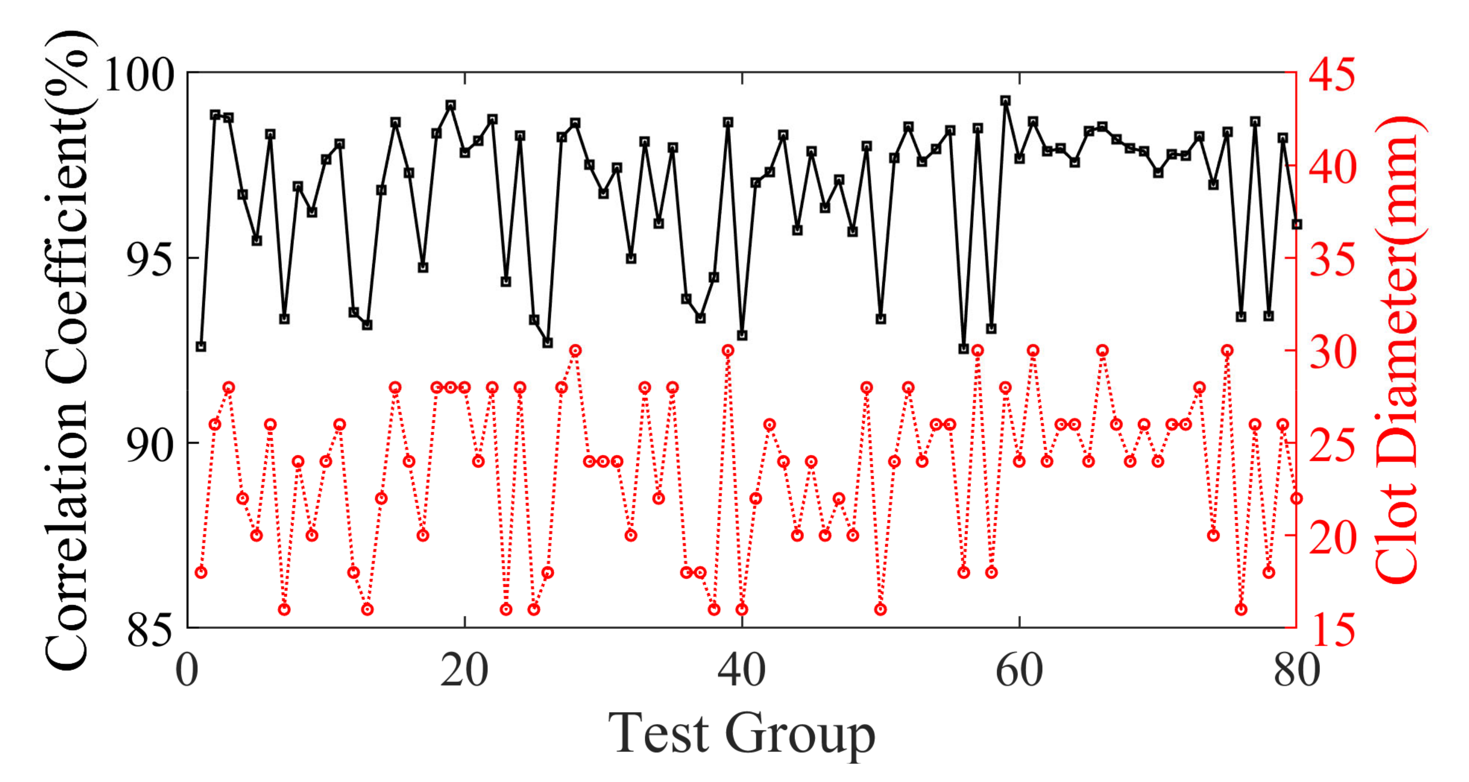
| Clot Size | Quantity | Average PC |
|---|---|---|
| 16–20 mm | 24 | 98.24415% |
| 21–26 mm | 43 | 98.57684% |
| >26 mm | 20 | 98.63558% |
| Skull | Data Size | Acoustic velocity |
| 256 mm × 300 mm × 200 mm | 2618 m/s | |
| Array | Number | Center frequency |
| 512 | 700 kHz | |
| Clot | Diameter | Velocity |
| 50 mm | 2222 m/s | |
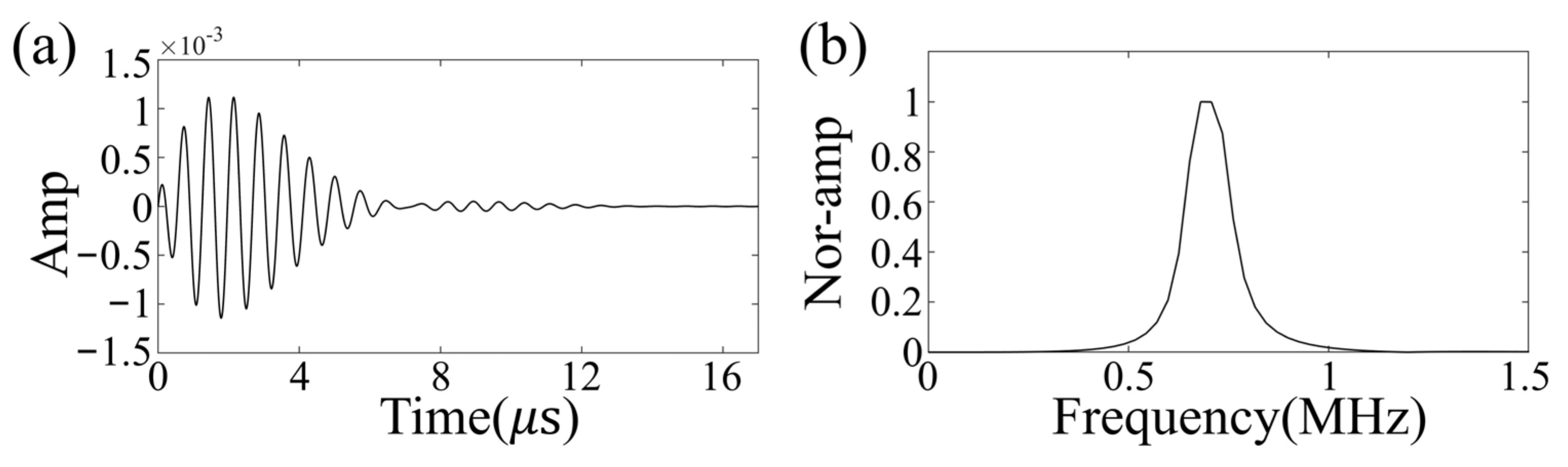
| Excitation | Type | Frequency |
| Ricker wavelet | 700 kHz |
Disclaimer/Publisher’s Note: The statements, opinions and data contained in all publications are solely those of the individual author(s) and contributor(s) and not of MDPI and/or the editor(s). MDPI and/or the editor(s) disclaim responsibility for any injury to people or property resulting from any ideas, methods, instructions or products referred to in the content. |
© 2023 by the authors. Licensee MDPI, Basel, Switzerland. This article is an open access article distributed under the terms and conditions of the Creative Commons Attribution (CC BY) license (https://creativecommons.org/licenses/by/4.0/).
Share and Cite
Ren, J.; Wang, X.; Liu, C.; Sun, H.; Tong, J.; Lin, M.; Li, J.; Liang, L.; Yin, F.; Xie, M.; et al. 3D Ultrasonic Brain Imaging with Deep Learning Based on Fully Convolutional Networks. Sensors 2023, 23, 8341. https://doi.org/10.3390/s23198341
Ren J, Wang X, Liu C, Sun H, Tong J, Lin M, Li J, Liang L, Yin F, Xie M, et al. 3D Ultrasonic Brain Imaging with Deep Learning Based on Fully Convolutional Networks. Sensors. 2023; 23(19):8341. https://doi.org/10.3390/s23198341
Chicago/Turabian StyleRen, Jiahao, Xiaocen Wang, Chang Liu, He Sun, Junkai Tong, Min Lin, Jian Li, Lin Liang, Feng Yin, Mengying Xie, and et al. 2023. "3D Ultrasonic Brain Imaging with Deep Learning Based on Fully Convolutional Networks" Sensors 23, no. 19: 8341. https://doi.org/10.3390/s23198341
APA StyleRen, J., Wang, X., Liu, C., Sun, H., Tong, J., Lin, M., Li, J., Liang, L., Yin, F., Xie, M., & Liu, Y. (2023). 3D Ultrasonic Brain Imaging with Deep Learning Based on Fully Convolutional Networks. Sensors, 23(19), 8341. https://doi.org/10.3390/s23198341