
A Simple Approach to Determine Single-Receiver Differential Code Bias Using Precise Point Positioning


Abstract
:1. Introduction
2. Methods and Data
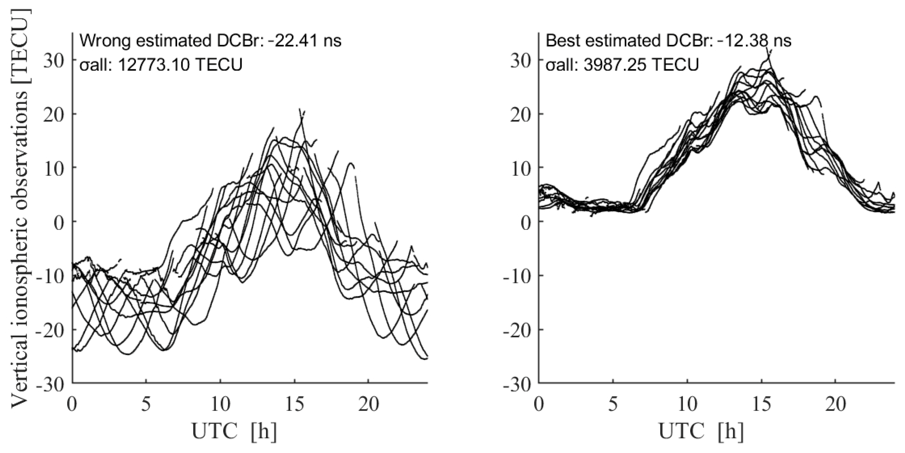
2.1. Methods
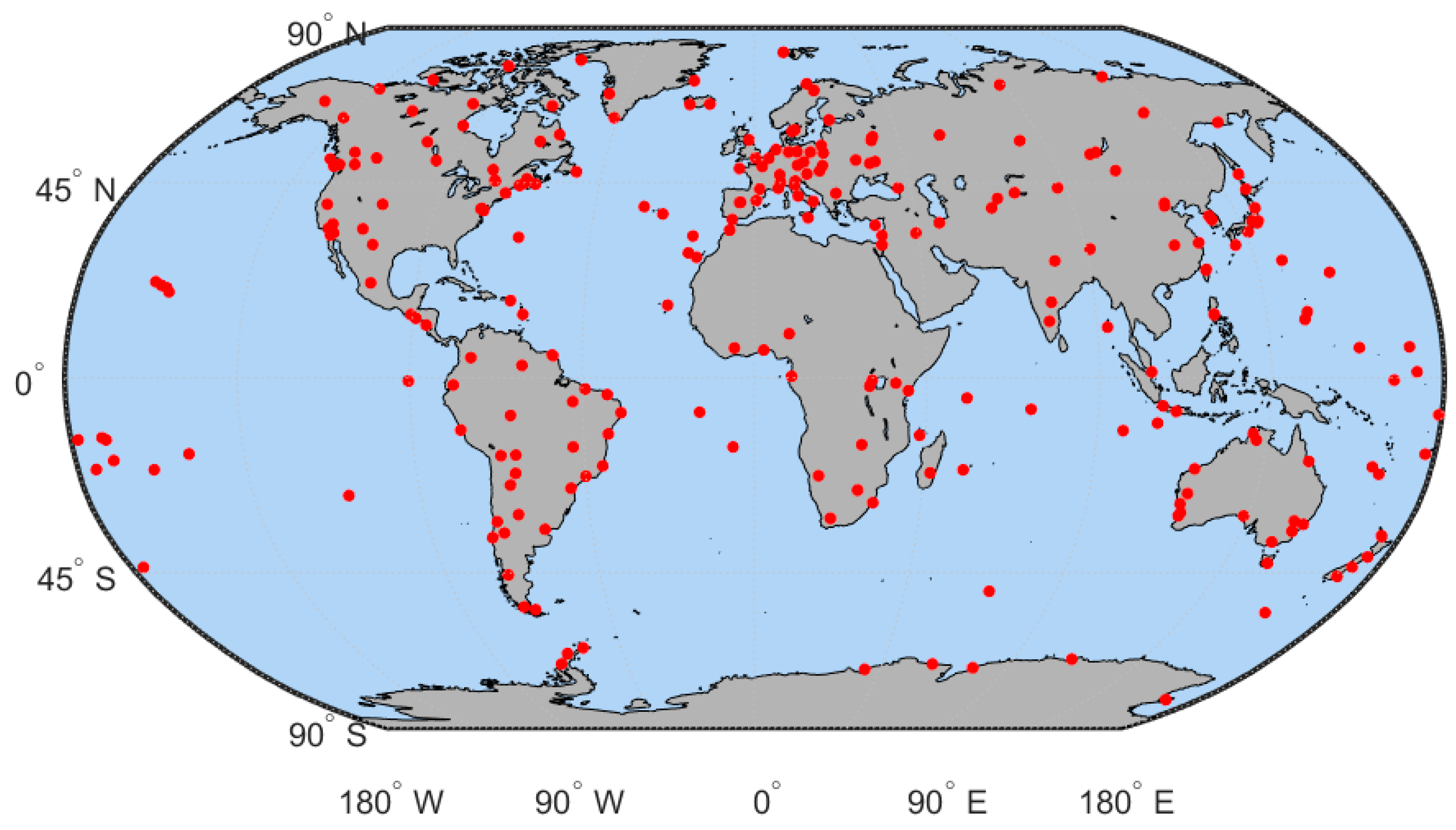
2.2. Data
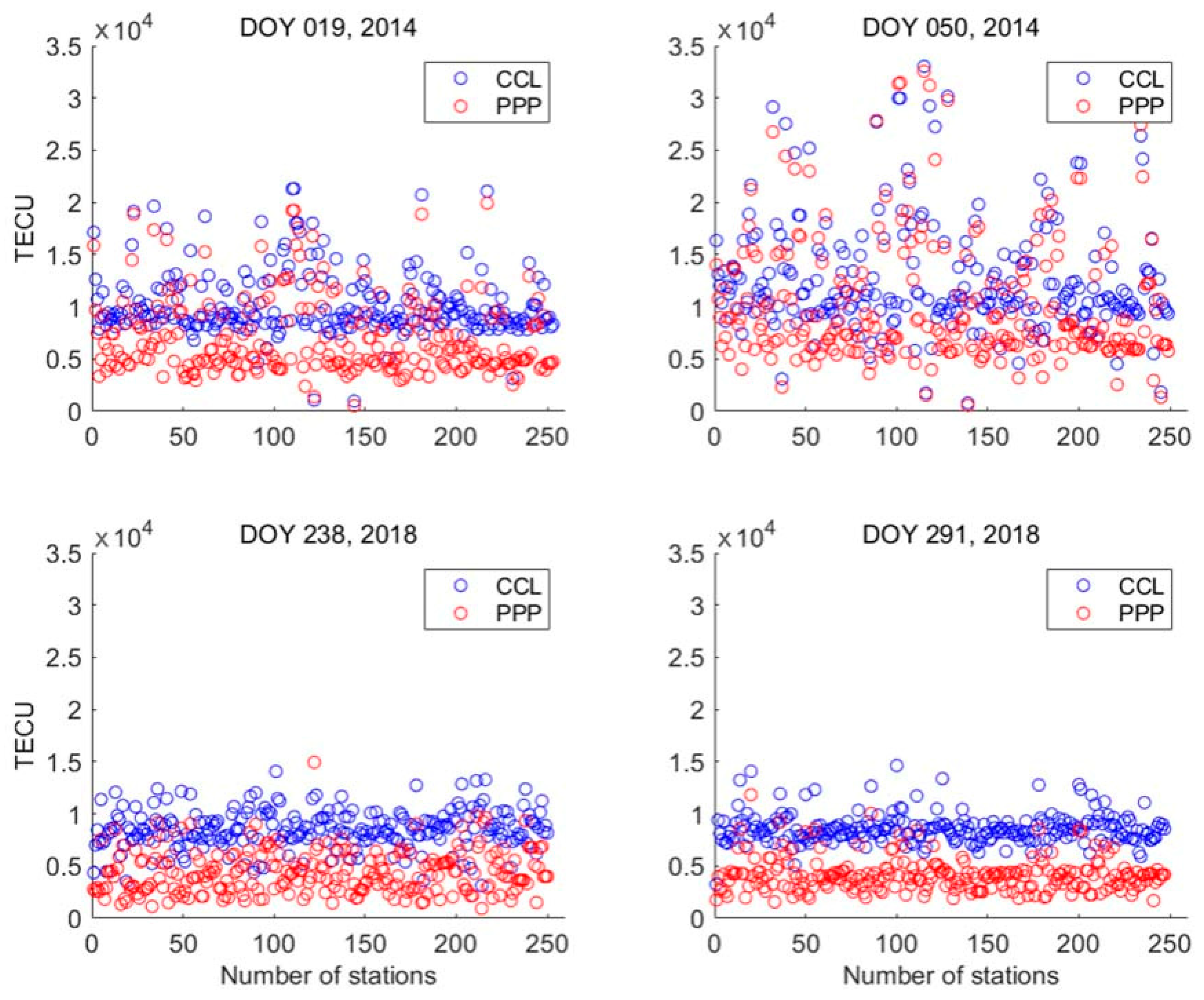
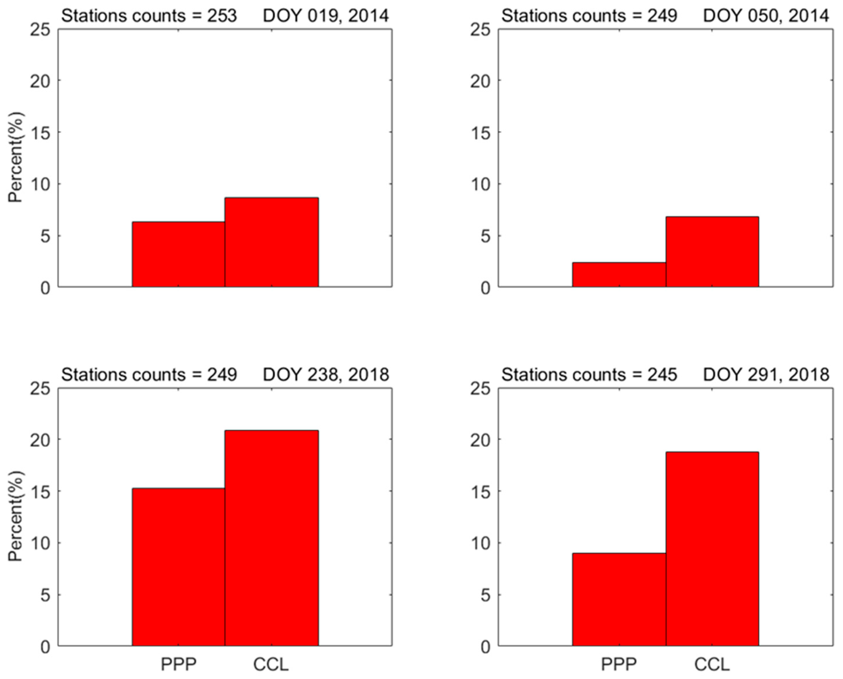
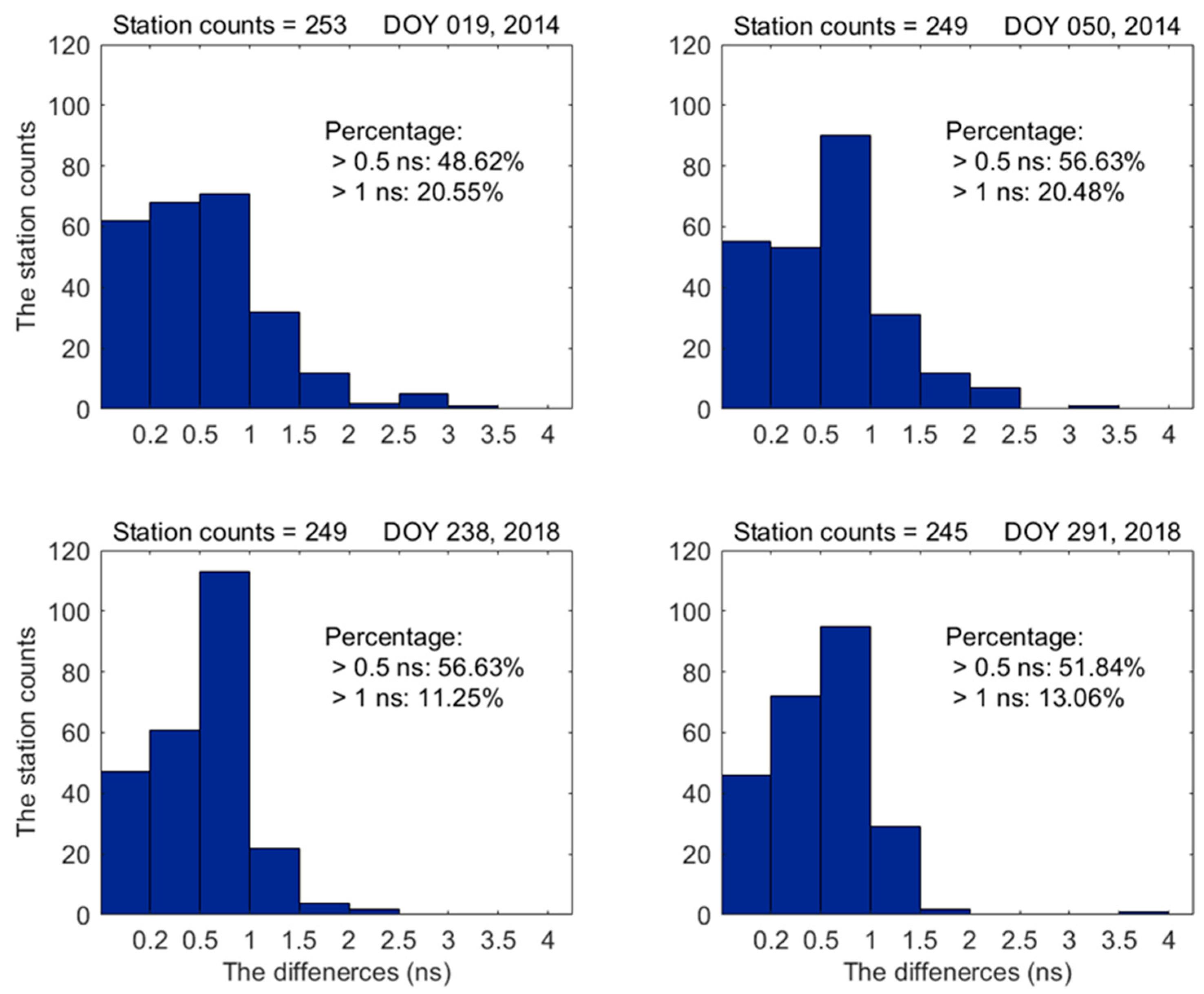
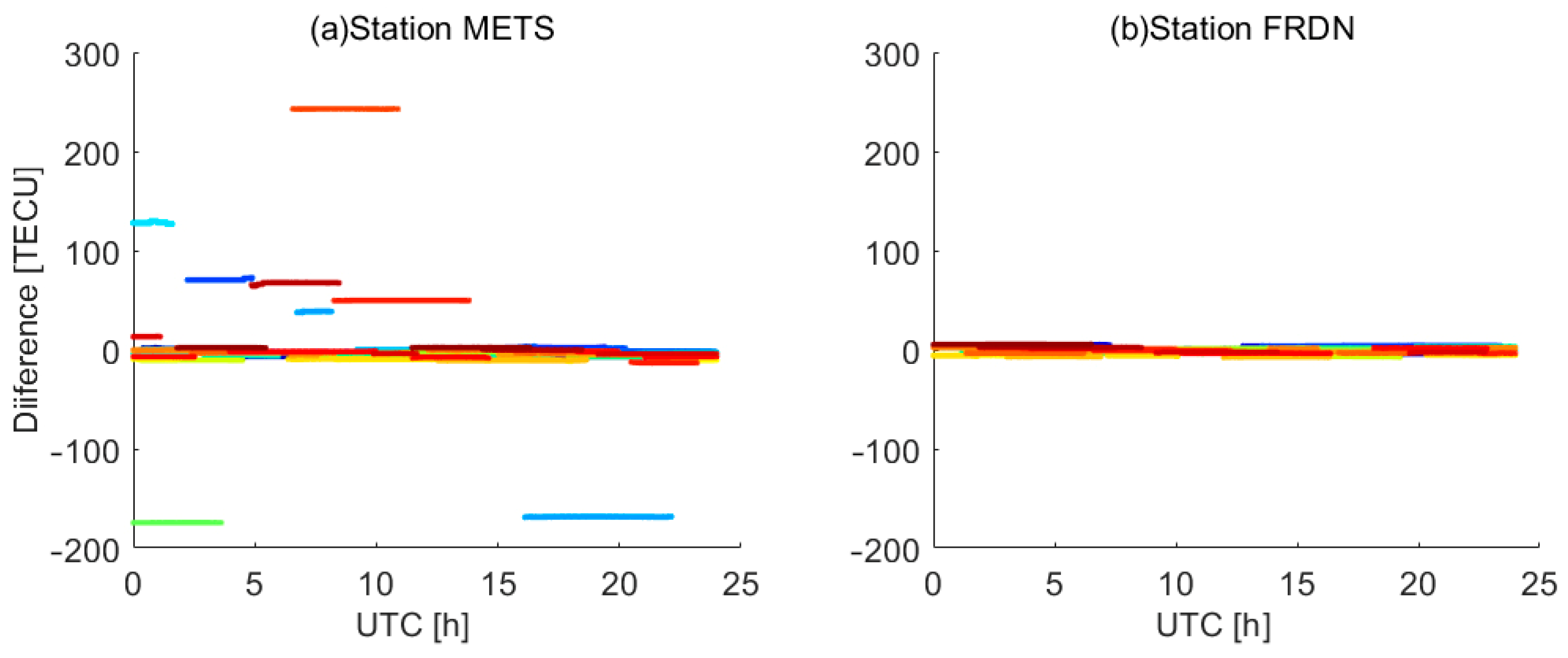
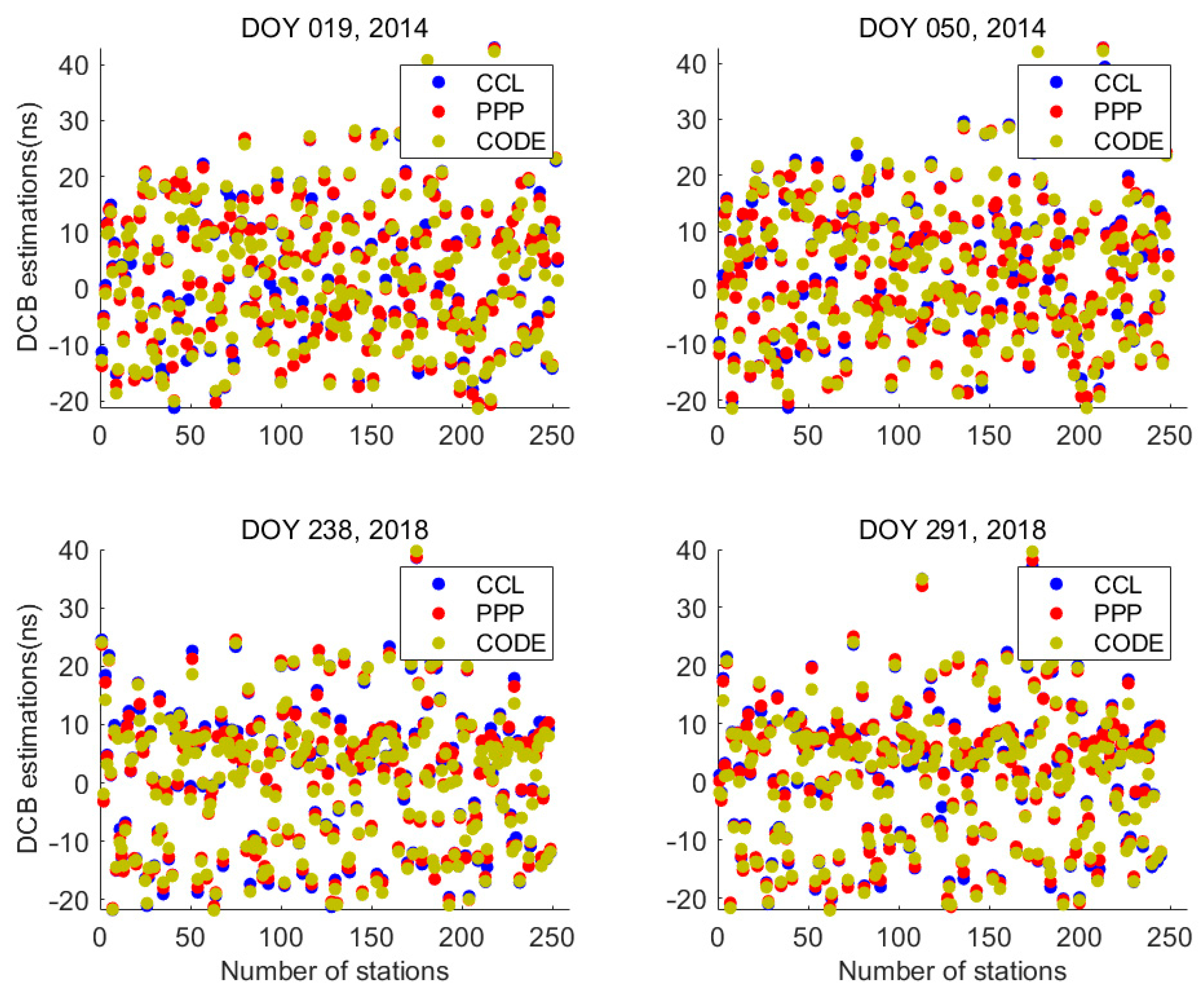
3. Results and Discussion
4. Conclusions and Perspectives
Author Contributions
Funding
Informed Consent Statement
Data Availability Statement
Acknowledgments
Conflicts of Interest
References
- Sardon, E.; Rius, A.; Zarraoa, N. Estimation of the transmitter and receiver differential biases and the ionospheric total electron content from Global Positioning System observations. Radio Sci. 1994, 29, 577–586. [Google Scholar] [CrossRef]
- Håkansson, M.; Jensen, A.B.; Horemuz, M.; Hedling, G. Review of code and phase biases in multi-GNSS positioning. GPS Solut. 2017, 21, 849–860. [Google Scholar] [CrossRef]
- Jensen, A.B.O.; Ovstedal, O.; Grinde, G. Development of a regional ionosphere model for Norway. In Proceedings of the International Technical Meeting of the Satellite Division of the Institute of Navigation, Fort Worth, TX, USA, 25–28 September 2007. [Google Scholar]
- Montenbruck, O.; Hauschild, A. Code biases in multi-GNSS point positioning. In Proceedings of the ION-ITM-2013, San Diego, CA, USA, 28–30 January 2013. [Google Scholar]
- Hernández-Pajares, M.; Juan, J.M.; Sanz, J.; Orus, R.; Garcia-Rigo, A.; Feltens, J.; Komjathy, A.; Schaer, S.C.; Krankowski, A. The IGS VTEC maps: A reliable source of ionospheric information since 1998. J. Geod. 2009, 83, 263–275. [Google Scholar] [CrossRef]
- Schaer, S. Mapping and Predicting the Earth’s Ionosphere Using the Global Positioning System; Technische Hochschule Zürich: Zürich, Switzerland, 1999; Volume 59. [Google Scholar]
- Li, Z.; Yuan, Y.; Li, H.; Ou, J.; Huo, X. Two-step method for the determination of the differential code biases of COMPASS satellites. J. Geod. 2012, 86, 1059–1076. [Google Scholar] [CrossRef]
- Arikan, F.; Nayir, H.; Sezen, U.; Arikan, O. Estimation of single station interfrequency receiver bias using GPS-TEC. Radio Sci. 2008, 43, 1–13. [Google Scholar] [CrossRef]
- Keshin, M. A new algorithm for single receiver DCB estimation using IGS TEC maps. GPS Solut. 2012, 16, 283–292. [Google Scholar] [CrossRef]
- Ma, G.; Maruyama, T. Derivation of TEC and estimation of instrumental biases from GEONET in Japan. Ann. Geophys. 2003, 21, 2083–2093. [Google Scholar] [CrossRef]
- Ciraolo, L.; Azpilicueta, F.; Brunini, C.; Meza, A.; Radicella, S.M. Calibration errors on experimental slant total electron content (TEC) determined with GPS. J. Geod. 2007, 81, 111–120. [Google Scholar] [CrossRef]
- Zhang, B.; Ou, J.; Yuan, Y.; Li, Z. Extraction of line-of-sight ionospheric observables from GPS data using precise point positioning. Sci. China Earth Sci. 2012, 55, 1919–1928. [Google Scholar] [CrossRef]
- Xiang, Y.; Gao, Y.; Shi, J.; Xu, C. Consistency and analysis of ionospheric observables obtained from three precise point positioning models. J. Geod. 2019, 93, 1161–1170. [Google Scholar] [CrossRef]
- Zhang, B. Three methods to retrieve slant total electron content measurements from ground-based GPS receivers and performance assessment. Radio Sci. 2016, 51, 972–988. [Google Scholar] [CrossRef]
- Liu, T.; Zhang, B.; Yuan, Y.; Li, Z.; Wang, N. Multi-GNSS triple-frequency differential code bias (DCB) determination with precise point positioning (PPP). J. Geod. 2019, 93, 765–784. [Google Scholar] [CrossRef]
- Zhou, P.; Nie, Z.; Xiang, Y.; Wang, J.; Du, L.; Gao, Y. Differential code bias estimation based on uncombined PPP with LEO onboard GPS observations. Adv. Space Res. 2020, 65, 541–551. [Google Scholar] [CrossRef]
- Wang, J.; Huang, G.; Zhou, P.; Yang, Y.; Zhang, Q.; Gao, Y. Advantages of Uncombined Precise Point Positioning with Fixed Ambiguity Resolution for Slant Total Electron Content (STEC) and Differential Code Bias (DCB) Estimation. Remote Sens. 2020, 12, 304. [Google Scholar] [CrossRef]
- Li, P.; Cui, B.; Hu, J.; Liu, X.; Zhang, X.; Ge, M.; Schuh, H. PPP-RTK considering the ionosphere uncertainty with cross-validation. Satell. Navig. 2022, 3, 1–13. [Google Scholar] [CrossRef]
- Yasyukevich, Y.V.; Mylnikova, A.A.; Polyakova, A.S. Estimating the total electron content absolute value from the GPS/GLONASS data. Results Phys. 2015, 5, 32–33. [Google Scholar] [CrossRef]
- Yasyukevich, Y.V.; Mylnikova, A.; Vesnin, A. GNSS-based non-negative absolute ionosphere total electron content, its spatial gradients, time derivatives and differential code biases: Bounded-variable least-squares and taylor series. Sensors 2020, 20, 5702. [Google Scholar] [CrossRef] [PubMed]
- Li, M.; Yuan, Y.; Wang, N.; Liu, T.; Chen, Y. Estimation and analysis of the short-term variations of multi-GNSS receiver differential code biases using global ionosphere maps. J. Geod. 2018, 92, 889–903. [Google Scholar] [CrossRef]

| Year | DOY | F10.7 | AE | Dst Index (nT) |
|---|---|---|---|---|
| 2014 | 019 | 123.4 | 26 | 8 |
| 2014 | 050 | 154.2 | 443 | −66 |
| 2018 | 238 | 72.6 | 692 | −104 |
| 2018 | 291 | 69.0 | 20 | −2 |
| Year | DOY | PPP (TECU) | CCL (TECU) | PPP–CCL (TECU) |
|---|---|---|---|---|
| 2014 | 019 | 6956.09 | 10,199.93 | −3243.84 |
| 2014 | 050 | 10,193.44 | 12,752.69 | −2559.24 |
| 2018 | 238 | 4382.26 | 8829.41 | −4447.16 |
| 2018 | 291 | 4136.07 | 8700.66 | −4564.58 |
| Year | DOY | Mean (ns) | Minimum (ns) | Maximum (ns) |
|---|---|---|---|---|
| 2014 | 019 | 0.640 | 0.002 | 3.263 |
| 2014 | 050 | 0.657 | 0.004 | 3.174 |
| 2018 | 238 | 0.584 | 0.005 | 2.437 |
| 2018 | 291 | 0.562 | 0.003 | 3.753 |
| Year | DOY | Mean (ns) | Minimum (ns) | Maximum (ns) | |||
|---|---|---|---|---|---|---|---|
| CCL | PPP | CCL | PPP | CCL | PPP | ||
| 2014 | 019 | −0.686 | −0.491 | −5.349 | −5.034 | 6.308 | 4.252 |
| 2014 | 050 | −0.348 | −0.347 | −5.357 | −5.697 | 7.640 | 7.019 |
| 2018 | 238 | −0.596 | −0.502 | −5.074 | −4.862 | 3.041 | 2.954 |
| 2018 | 291 | −0.617 | −0.587 | −4.992 | −4.660 | 3.693 | 2.117 |
Disclaimer/Publisher’s Note: The statements, opinions and data contained in all publications are solely those of the individual author(s) and contributor(s) and not of MDPI and/or the editor(s). MDPI and/or the editor(s) disclaim responsibility for any injury to people or property resulting from any ideas, methods, instructions or products referred to in the content. |
© 2023 by the authors. Licensee MDPI, Basel, Switzerland. This article is an open access article distributed under the terms and conditions of the Creative Commons Attribution (CC BY) license (https://creativecommons.org/licenses/by/4.0/).
Share and Cite
Zhang, F.; Tang, L.; Li, J.; Du, X. A Simple Approach to Determine Single-Receiver Differential Code Bias Using Precise Point Positioning. Sensors 2023, 23, 8230. https://doi.org/10.3390/s23198230
Zhang F, Tang L, Li J, Du X. A Simple Approach to Determine Single-Receiver Differential Code Bias Using Precise Point Positioning. Sensors. 2023; 23(19):8230. https://doi.org/10.3390/s23198230
Chicago/Turabian StyleZhang, Fenkai, Long Tang, Jiaxing Li, and Xiangfeng Du. 2023. "A Simple Approach to Determine Single-Receiver Differential Code Bias Using Precise Point Positioning" Sensors 23, no. 19: 8230. https://doi.org/10.3390/s23198230
APA StyleZhang, F., Tang, L., Li, J., & Du, X. (2023). A Simple Approach to Determine Single-Receiver Differential Code Bias Using Precise Point Positioning. Sensors, 23(19), 8230. https://doi.org/10.3390/s23198230