
Unsupervised Spiking Neural Network with Dynamic Learning of Inhibitory Neurons

 , , and
Abstract
:1. Introduction
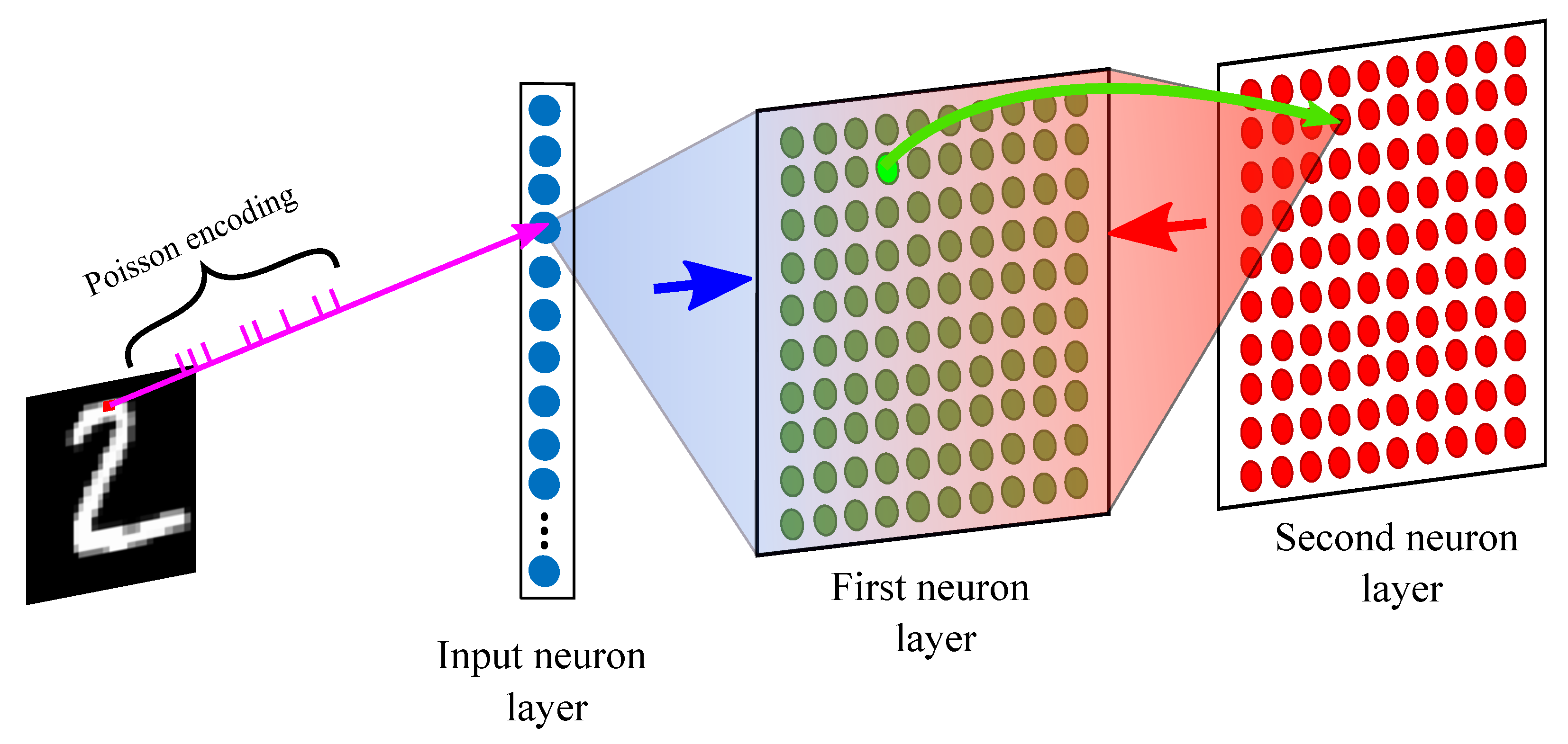
2. Network Architecture
2.1. Input Neuron Layer
STDP
2.2. First Neuron Layer
2.3. Second Neuron Layer
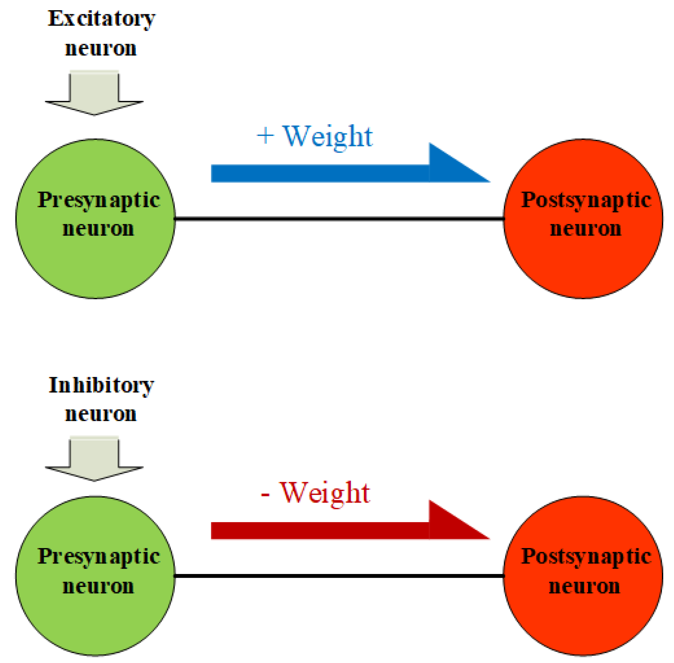
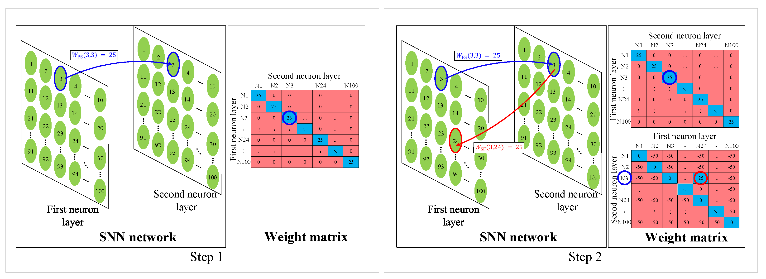
2.3.1. Inhibition Weight Update
| Algorithm 1 Inhibition Weight Update and Synaptic Wiring |
|
2.3.2. Synaptic Wiring
2.4. Inference
3. Results
4. Discussion
4.1. Inhibitory Neurons
4.2. Synapse
4.3. Biological Inference
5. Conclusions
Author Contributions
Funding
Institutional Review Board Statement
Informed Consent Statement
Data Availability Statement
Conflicts of Interest
References
- Maass, W. Networks of spiking neurons: The third generation of neural network models. Neural Netw. 1997, 10, 1659–1671. [Google Scholar] [CrossRef]
- Hinton, G.E.; Salakhutdinov, R.R. Reducing the dimensionality of data with neural networks. Science 2006, 313, 504–507. [Google Scholar] [CrossRef] [PubMed]
- Han, J.; Choi, J.; Lee, C. Image Denoising Method based on Deep Learning using Improved U-net. IEIE Trans. Smart Process. Comput. 2021, 10, 291–295. [Google Scholar] [CrossRef]
- Rashed-Al-Mahfuz, M.; Moni, M.A.; Lio, P.; Islam, S.M.S.; Berkovsky, S.; Khushi, M.; Quinn, J.M. Deep convolutional neural networks based ECG beats classification to diagnose cardiovascular conditions. Biomed. Eng. Lett. 2021, 11, 147–162. [Google Scholar] [CrossRef]
- O’reilly, R.C.; Munakata, Y. Computational Explorations in Cognitive Neuroscience: Understanding the Mind by Simulating the Brain; MIT Press: Cambridge, MA, USA, 2000. [Google Scholar]
- Demin, V.; Nekhaev, D. Recurrent spiking neural network learning based on a competitive maximization of neuronal activity. Front. Neuroinform. 2018, 12, 79. [Google Scholar] [CrossRef]
- Hodgkin, A.L.; Huxley, A.F. A quantitative description of membrane current and its application to conduction and excitation in nerve. J. Physiol. 1952, 117, 500. [Google Scholar] [CrossRef]
- Izhikevich, E.M. Simple model of spiking neurons. IEEE Trans. Neural Netw. 2003, 14, 1569–1572. [Google Scholar] [CrossRef]
- Burkitt, A.N. A review of the integrate-and-fire neuron model: I. Homogeneous synaptic input. Biol. Cybern. 2006, 95, 1–19. [Google Scholar] [CrossRef]
- Bienenstock, E.L.; Cooper, L.N.; Munro, P.W. Theory for the development of neuron selectivity: Orientation specificity and binocular interaction in visual cortex. J. Neurosci. 1982, 2, 32–48. [Google Scholar] [CrossRef]
- Izhikevich, E.M.; Desai, N.S. Relating stdp to bcm. Neural Comput. 2003, 15, 1511–1523. [Google Scholar] [CrossRef]
- Auge, D.; Hille, J.; Mueller, E.; Knoll, A. A survey of encoding techniques for signal processing in spiking neural networks. Neural Process. Lett. 2021, 53, 4693–4710. [Google Scholar] [CrossRef]
- Sboev, A.; Vlasov, D.; Rybka, R.; Serenko, A. Solving a classification task by spiking neurons with STDP and temporal coding. Procedia Comput. Sci. 2018, 123, 494–500. [Google Scholar] [CrossRef]
- Merolla, P.; Arthur, J.; Akopyan, F.; Imam, N.; Manohar, R.; Modha, D.S. A digital neurosynaptic core using embedded crossbar memory with 45 pJ per spike in 45 nm. In Proceedings of the 2011 IEEE Custom Integrated Circuits Conference (CICC), San Jose, CA, USA, 19–21 September 2011; IEEE: Piscataway, NJ, USA, 2011; pp. 1–4. [Google Scholar]
- Hussain, S.; Liu, S.C.; Basu, A. Improved margin multi-class classification using dendritic neurons with morphological learning. In Proceedings of the 2014 IEEE International Symposium on Circuits and Systems (ISCAS), Melbourne, Australia, 1–5 June 2014; IEEE: Piscataway, NJ, USA, 2014; pp. 2640–2643. [Google Scholar]
- Neil, D.; Liu, S.C. Minitaur, an event-driven FPGA-based spiking network accelerator. IEEE Trans. Very Large Scale Integr. (VLSI) Syst. 2014, 22, 2621–2628. [Google Scholar] [CrossRef]
- Zhong, Y.; Huang, X. A Painting Style System using an Improved CNN Algorithm. IEIE Trans. Smart Process. Comput. 2022, 11, 332–342. [Google Scholar] [CrossRef]
- Tavanaei, A.; Kirby, Z.; Maida, A.S. Training spiking convnets by stdp and gradient descent. In Proceedings of the 2018 International Joint Conference on Neural Networks (IJCNN), Rio de Janeiro, Brazil, 8–13 July 2018; IEEE: Piscataway, NJ, USA, 2018; pp. 1–8. [Google Scholar]
- Rueckauer, B.; Lungu, I.A.; Hu, Y.; Pfeiffer, M.; Liu, S.C. Conversion of continuous-valued deep networks to efficient event-driven networks for image classification. Front. Neurosci. 2017, 11, 682. [Google Scholar] [CrossRef]
- Brader, J.M.; Senn, W.; Fusi, S. Learning real-world stimuli in a neural network with spike-driven synaptic dynamics. Neural Comput. 2007, 19, 2881–2912. [Google Scholar] [CrossRef]
- Bohte, S.M.; Kok, J.N.; La Poutré, J.A. SpikeProp: Backpropagation for networks of spiking neurons. In Proceedings of the ESANN, Bruges, Belgium, 26–28 April 2000; Volume 48, pp. 419–424. [Google Scholar]
- Sacramento, J.; Ponte Costa, R.; Bengio, Y.; Senn, W. Dendritic cortical microcircuits approximate the backpropagation algorithm. In Proceedings of the Advances in Neural Information Processing Systems, Montreal, QC, Canada, 3–8 December 2018; Volume 31. [Google Scholar]
- Friston, K.; Kilner, J.; Harrison, L. A free energy principle for the brain. J. Physiol.-Paris 2006, 100, 70–87. [Google Scholar] [CrossRef]
- Rao, R.P.; Ballard, D.H. Predictive coding in the visual cortex: A functional interpretation of some extra-classical receptive-field effects. Nat. Neurosci. 1999, 2, 79–87. [Google Scholar] [CrossRef]
- Zador, A.M. A critique of pure learning and what artificial neural networks can learn from animal brains. Nat. Commun. 2019, 10, 3770. [Google Scholar] [CrossRef]
- Krotov, D.; Hopfield, J.J. Unsupervised learning by competing hidden units. Proc. Natl. Acad. Sci. USA 2019, 116, 7723–7731. [Google Scholar] [CrossRef]
- Khacef, L.; Rodriguez, L.; Miramond, B. Brain-inspired self-organization with cellular neuromorphic computing for multimodal unsupervised learning. Electronics 2020, 9, 1605. [Google Scholar] [CrossRef]
- Kohonen, T.; Kaski, S.; Lagus, K.; Salojarvi, J.; Honkela, J.; Paatero, V.; Saarela, A. Self organization of a massive document collection. IEEE Trans. Neural Netw. 2000, 11, 574–585. [Google Scholar] [CrossRef]
- She, X.; Dash, S.; Kim, D.; Mukhopadhyay, S. A heterogeneous spiking neural network for unsupervised learning of spatiotemporal patterns. Front. Neurosci. 2021, 14, 1406. [Google Scholar] [CrossRef] [PubMed]
- Hebb, D.O. The Organization of Behavior: A Neuropsychological Theory; Psychology Press: London, UK, 2005. [Google Scholar]
- Cooke, S.F.; Bliss, T.V. Plasticity in the human central nervous system. Brain 2006, 129, 1659–1673. [Google Scholar] [CrossRef]
- Kohn, A.; Coen-Cagli, R.; Kanitscheider, I.; Pouget, A. Correlations and neuronal population information. Annu. Rev. Neurosci. 2016, 39, 237–256. [Google Scholar] [CrossRef] [PubMed]
- Sanger, T.D. Neural population codes. Curr. Opin. Neurobiol. 2003, 13, 238–249. [Google Scholar] [CrossRef] [PubMed]
- Diehl, P.U.; Cook, M. Unsupervised learning of digit recognition using spike-timing-dependent plasticity. Front. Comput. Neurosci. 2015, 9, 99. [Google Scholar] [CrossRef]
- LeCun, Y. The MNIST Database of Handwritten Digits. Available online: http://yann.lecun.com/exdb/mnist/ (accessed on 19 October 2018).
- Cohen, G.; Afshar, S.; Tapson, J.; Van Schaik, A. EMNIST: Extending MNIST to handwritten letters. In Proceedings of the 2017 International Joint Conference on Neural Networks (IJCNN), Anchorage, AK, USA, 14–19 May 2017; IEEE: Piscataway, NJ, USA, 2017; pp. 2921–2926. [Google Scholar]
- Zhang, J. Basic neural units of the brain: Neurons, synapses and action potential. arXiv 2019, arXiv:1906.01703. [Google Scholar]
- Deneve, S. Bayesian inference in spiking neurons. In Proceedings of the Advances in Neural Information Processing Systems, Vancouver, BC, Canada, 13–18 December 2004; Volume 17. [Google Scholar]
- Körding, K.P.; Wolpert, D.M. Bayesian decision theory in sensorimotor control. Trends Cogn. Sci. 2006, 10, 319–326. [Google Scholar] [CrossRef]
- Kording, K. Decision theory: What “should” the nervous system do? Science 2007, 318, 606–610. [Google Scholar] [CrossRef]
- Laurens, J.; Droulez, J. Bayesian processing of vestibular information. Biol. Cybern. 2007, 96, 389–404. [Google Scholar] [CrossRef] [PubMed]
- Stevenson, I.H.; Fernandes, H.L.; Vilares, I.; Wei, K.; Körding, K.P. Bayesian integration and non-linear feedback control in a full-body motor task. PLoS Comput. Biol. 2009, 5, e1000629. [Google Scholar] [CrossRef] [PubMed]
- Pouget, A.; Beck, J.M.; Ma, W.J.; Latham, P.E. Probabilistic brains: Knowns and unknowns. Nat. Neurosci. 2013, 16, 1170–1178. [Google Scholar] [CrossRef] [PubMed]
- Hazan, H.; Saunders, D.J.; Khan, H.; Patel, D.; Sanghavi, D.T.; Siegelmann, H.T.; Kozma, R. Bindsnet: A machine learning-oriented spiking neural networks library in python. Front. Neuroinform. 2018, 12, 89. [Google Scholar] [CrossRef]
- Gerstner, W.; Kistler, W.M. Spiking Neuron Models: Single Neurons, Populations, Plasticity; Cambridge University Press: Cambridge, UK, 2002. [Google Scholar]
- Tavanaei, A.; Ghodrati, M.; Kheradpisheh, S.R.; Masquelier, T.; Maida, A. Deep learning in spiking neural networks. Neural Netw. 2019, 111, 47–63. [Google Scholar] [CrossRef]
- Yang, J.Q.; Wang, R.; Wang, Z.P.; Ma, Q.Y.; Mao, J.Y.; Ren, Y.; Yang, X.; Zhou, Y.; Han, S.T. Leaky integrate-and-fire neurons based on perovskite memristor for spiking neural networks. Nano Energy 2020, 74, 104828. [Google Scholar] [CrossRef]
- Jaiswal, A.; Roy, S.; Srinivasan, G.; Roy, K. Proposal for a leaky-integrate-fire spiking neuron based on magnetoelectric switching of ferromagnets. IEEE Trans. Electron. Devices 2017, 64, 1818–1824. [Google Scholar] [CrossRef]
- Finkelstein, A.; Hetherington, J.; Li, L.; Margoninski, O.; Saffrey, P.; Seymour, R.; Warner, A. Computational challenges of systems biology. Computer 2004, 37, 26–33. [Google Scholar] [CrossRef]
- Gerstner, W.; Kistler, W.M.; Naud, R.; Paninski, L. Neuronal Dynamics: From Single Neurons to Networks and Models of Cognition; Cambridge University Press: Cambridge, UK, 2014. [Google Scholar]
- Bi, G.q.; Poo, M.m. Synaptic modifications in cultured hippocampal neurons: Dependence on spike timing, synaptic strength, and postsynaptic cell type. J. Neurosci. 1998, 18, 10464–10472. [Google Scholar] [CrossRef]
- Saunders, D.J.; Patel, D.; Hazan, H.; Siegelmann, H.T.; Kozma, R. Locally connected spiking neural networks for unsupervised feature learning. Neural Netw. 2019, 119, 332–340. [Google Scholar] [CrossRef]
- Lodish, H.; Berk, A.; Zipursky, S.L.; Matsudaira, P.; Baltimore, D.; Darnell, J. Neurotransmitters, Synapses, and Impulse Transmission. In Molecular Cell Biology, 4th ed.; WH Freeman: New York, NY, USA, 2000. [Google Scholar]
- Vazquez, A.L.; Fukuda, M.; Kim, S.G. Inhibitory neuron activity contributions to hemodynamic responses and metabolic load examined using an inhibitory optogenetic mouse model. Cereb. Cortex 2018, 28, 4105–4119. [Google Scholar] [CrossRef] [PubMed]
- Carroll, B.J.; Bertram, R.; Hyson, R.L. Intrinsic physiology of inhibitory neurons changes over auditory development. J. Neurophysiol. 2018, 119, 290–304. [Google Scholar] [CrossRef] [PubMed]
- Chamberland, S.; Topolnik, L. Inhibitory control of hippocampal inhibitory neurons. Front. Neurosci. 2012, 6, 165. [Google Scholar] [CrossRef]
- Ruder, S. An overview of gradient descent optimization algorithms. arXiv 2016, arXiv:1609.04747. [Google Scholar]
- Baudry, M. Synaptic plasticity and learning and memory: 15 years of progress. Neurobiol. Learn. Mem. 1998, 70, 113–118. [Google Scholar] [CrossRef] [PubMed]
- Panzeri, S.; Macke, J.H.; Gross, J.; Kayser, C. Neural population coding: Combining insights from microscopic and mass signals. Trends Cogn. Sci. 2015, 19, 162–172. [Google Scholar] [CrossRef]
- Valencia, D.; Alimohammad, A. Towards in vivo neural decoding. Biomed. Eng. Lett. 2022, 12, 185–195. [Google Scholar] [CrossRef]
- Gerstner, W. Hebbian learning and plasticity. In From Neuron to Cognition via Computational Neuroscience; MIT Press: Cambridge, MA, USA, 2011; pp. 1–25. [Google Scholar]
- Zhang, W.; Linden, D.J. The other side of the engram: Experience-driven changes in neuronal intrinsic excitability. Nat. Rev. Neurosci. 2003, 4, 885–900. [Google Scholar] [CrossRef] [PubMed]
- Querlioz, D.; Bichler, O.; Dollfus, P.; Gamrat, C. Immunity to device variations in a spiking neural network with memristive nanodevices. IEEE Trans. Nanotechnol. 2013, 12, 288–295. [Google Scholar] [CrossRef]
- Rousselet, G.A.; Fabre-Thorpe, M.; Thorpe, S.J. Parallel processing in high-level categorization of natural images. Nat. Neurosci. 2002, 5, 629–630. [Google Scholar] [CrossRef]
- DiCarlo, J.J.; Zoccolan, D.; Rust, N.C. How does the brain solve visual object recognition? Neuron 2012, 73, 415–434. [Google Scholar] [CrossRef]
- Consul, P.C.; Jain, G.C. A generalization of the Poisson distribution. Technometrics 1973, 15, 791–799. [Google Scholar] [CrossRef]
- Hao, Y.; Huang, X.; Dong, M.; Xu, B. A biologically plausible supervised learning method for spiking neural networks using the symmetric STDP rule. Neural Netw. 2020, 121, 387–395. [Google Scholar] [CrossRef] [PubMed]
- Jonas, P.; Buzsaki, G. Neural inhibition. Scholarpedia 2007, 2, 3286. [Google Scholar] [CrossRef]
- Liu, Y.C.; Cheng, J.K.; Lien, C.C. Rapid dynamic changes of dendritic inhibition in the dentate gyrus by presynaptic activity patterns. J. Neurosci. 2014, 34, 1344–1357. [Google Scholar] [CrossRef] [PubMed]
- Widrow, B.; Kim, Y.; Park, D.; Perin, J.K. Nature’s learning rule: The Hebbian-LMS algorithm. In Artificial Intelligence in the Age of Neural Networks and Brain Computing; Elsevier: Amsterdam, The Netherlands, 2019; pp. 1–30. [Google Scholar]
- Fatahi, M.; Ahmadi, M.; Shahsavari, M.; Ahmadi, A.; Devienne, P. evt_MNIST: A spike based version of traditional MNIST. arXiv 2016, arXiv:1604.06751. [Google Scholar]


| Weight, | Accuracy (%, 1600 Neurons) |
|---|---|
| −36 | 88.51 |
| −37 | 88.20 |
| −38 | 92.30 |
| −39 | 90.15 |
| −40 | 91.25 |
| No. of Neurons | No. of Training Data Samples * | Accuracy (%) | No. of Synaptic Wirings |
|---|---|---|---|
| 200 | 6000 | 84.48 ± 0.17 | 23 |
| 400 | 10,000 | 87.25 ± 0.15 | 65 |
| 900 | 25,000 | 90.05 ± 0.13 | 112 |
| 1100 | 30,000 | 90.72 ± 0.13 | 124 |
| 1600 | 75,000 | 92.30 ± 0.14 | 241 |
| 3000 | 90,000 | 92.21 ± 0.10 | 273 |
| No. of Neurons | No. of Training Data Samples * | Accuracy (%) | No. of Synaptic Wirings |
|---|---|---|---|
| 200 | 20,000 | 81.20 ± 0.13 | 15 |
| 400 | 44,000 | 84.45 ± 0.15 | 56 |
| 900 | 90,000 | 87.35 ± 0.15 | 189 |
| 1100 | 96,000 | 88.20 ± 0.14 | 276 |
| 1600 | 102,000 | 88.70 ± 0.19 | 387 |
| 3000 | 114,000 | 90.04 ± 0.20 | 392 |
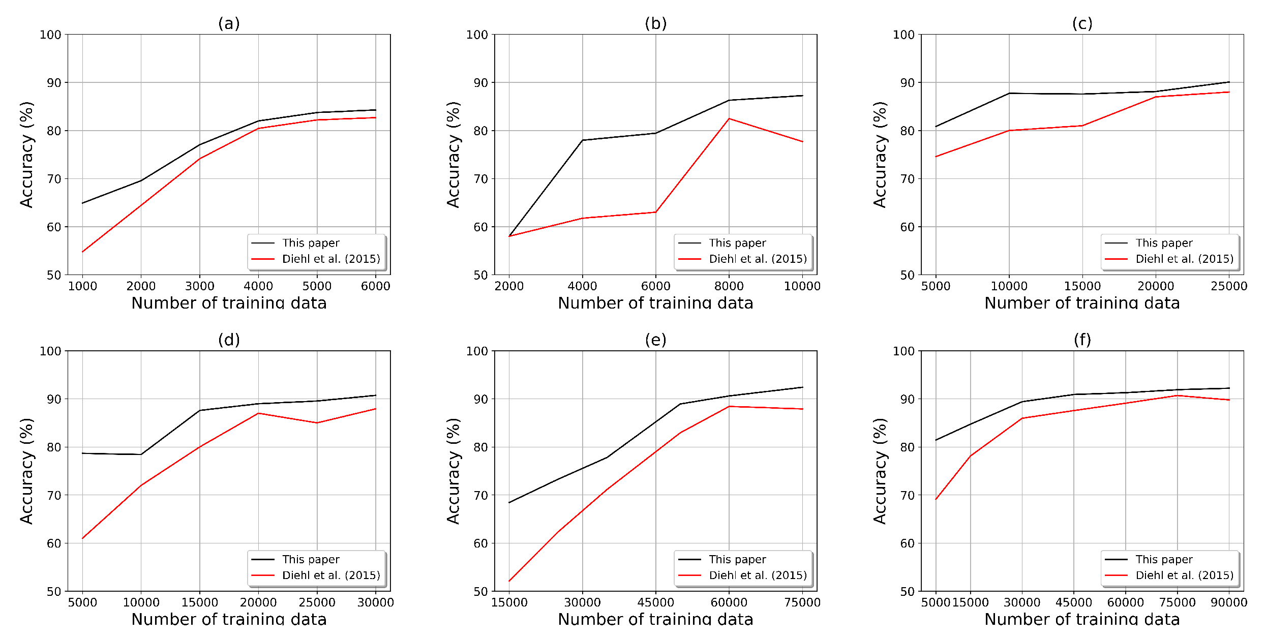
| No. of Neurons | Accuracy (%) for the MNIST Dataset | Accuracy (%) for the EMNIST Dataset | ||||
|---|---|---|---|---|---|---|
| Proposed Model | Diehl et al. (2015) [34] | Hao et al. (2020) [67] | Proposed Model | Diehl et al. (2015) [34] | Hao et al. (2020) [67] | |
| 200 | 84.48 ± 0.17 | 82.68 ± 0.18 | 78.56 ± 0.22 | 81.20 ± 0.13 | 78.08 ± 0.11 | 77.78 ± 0.12 |
| 400 | 87.25 ± 0.15 | 77.70 ± 0.20 | 87.18 ± 0.12 | 84.45 ± 0.15 | 82.01 ± 0.13 | 81.25 ± 0.11 |
| 900 | 90.05 ± 0.13 | 88.14 ± 0.17 | 86.85 ± 0.21 | 87.35 ± 0.15 | 83.83 ± 0.12 | 84.50 ± 0.14 |
| 1100 | 90.72 ± 0.13 | 87.92 ± 0.15 | 87.44 ± 0.11 | 88.20 ± 0.14 | 85.25 ± 0.13 | 86.17 ± 0.11 |
| 1600 | 92.30 ± 0.14 | 87.85 ± 0.14 | 88.60 ± 0.18 | 88.70 ± 0.19 | 87.90 ± 0.13 | 87.60 ± 0.12 |
| 3000 | 92.21 ± 0.10 | 89.77 ± 0.12 | 90.15 ± 0.10 | 90.04 ± 0.20 | 87.02 ± 0.11 | 87.75 ± 0.14 |
| Neurons | Training Samples | Accuracy (Gaussian) | Accuracy (Poisson) |
|---|---|---|---|
| 200 | 6000 | 50.74 ± 0.35 | 84.48 ± 0.17 |
| 400 | 10,000 | 61.90 ± 0.32 | 87.25 ± 0.15 |
| 900 | 25,000 | 73.99 ± 0.20 | 90.05 ± 0.13 |
| 1100 | 30,000 | 77.24 ± 0.30 | 90.72 ± 0.13 |
| 1600 | 75,000 | 80.65 ± 0.33 | 92.30 ± 0.14 |
| 3000 | 90,000 | 83.26 ± 0.27 | 92.21 ± 0.10 |
Disclaimer/Publisher’s Note: The statements, opinions and data contained in all publications are solely those of the individual author(s) and contributor(s) and not of MDPI and/or the editor(s). MDPI and/or the editor(s) disclaim responsibility for any injury to people or property resulting from any ideas, methods, instructions or products referred to in the content. |
© 2023 by the authors. Licensee MDPI, Basel, Switzerland. This article is an open access article distributed under the terms and conditions of the Creative Commons Attribution (CC BY) license (https://creativecommons.org/licenses/by/4.0/).
Share and Cite
Yang, G.; Lee, W.; Seo, Y.; Lee, C.; Seok, W.; Park, J.; Sim, D.; Park, C. Unsupervised Spiking Neural Network with Dynamic Learning of Inhibitory Neurons. Sensors 2023, 23, 7232. https://doi.org/10.3390/s23167232
Yang G, Lee W, Seo Y, Lee C, Seok W, Park J, Sim D, Park C. Unsupervised Spiking Neural Network with Dynamic Learning of Inhibitory Neurons. Sensors. 2023; 23(16):7232. https://doi.org/10.3390/s23167232
Chicago/Turabian StyleYang, Geunbo, Wongyu Lee, Youjung Seo, Choongseop Lee, Woojoon Seok, Jongkil Park, Donggyu Sim, and Cheolsoo Park. 2023. "Unsupervised Spiking Neural Network with Dynamic Learning of Inhibitory Neurons" Sensors 23, no. 16: 7232. https://doi.org/10.3390/s23167232
APA StyleYang, G., Lee, W., Seo, Y., Lee, C., Seok, W., Park, J., Sim, D., & Park, C. (2023). Unsupervised Spiking Neural Network with Dynamic Learning of Inhibitory Neurons. Sensors, 23(16), 7232. https://doi.org/10.3390/s23167232