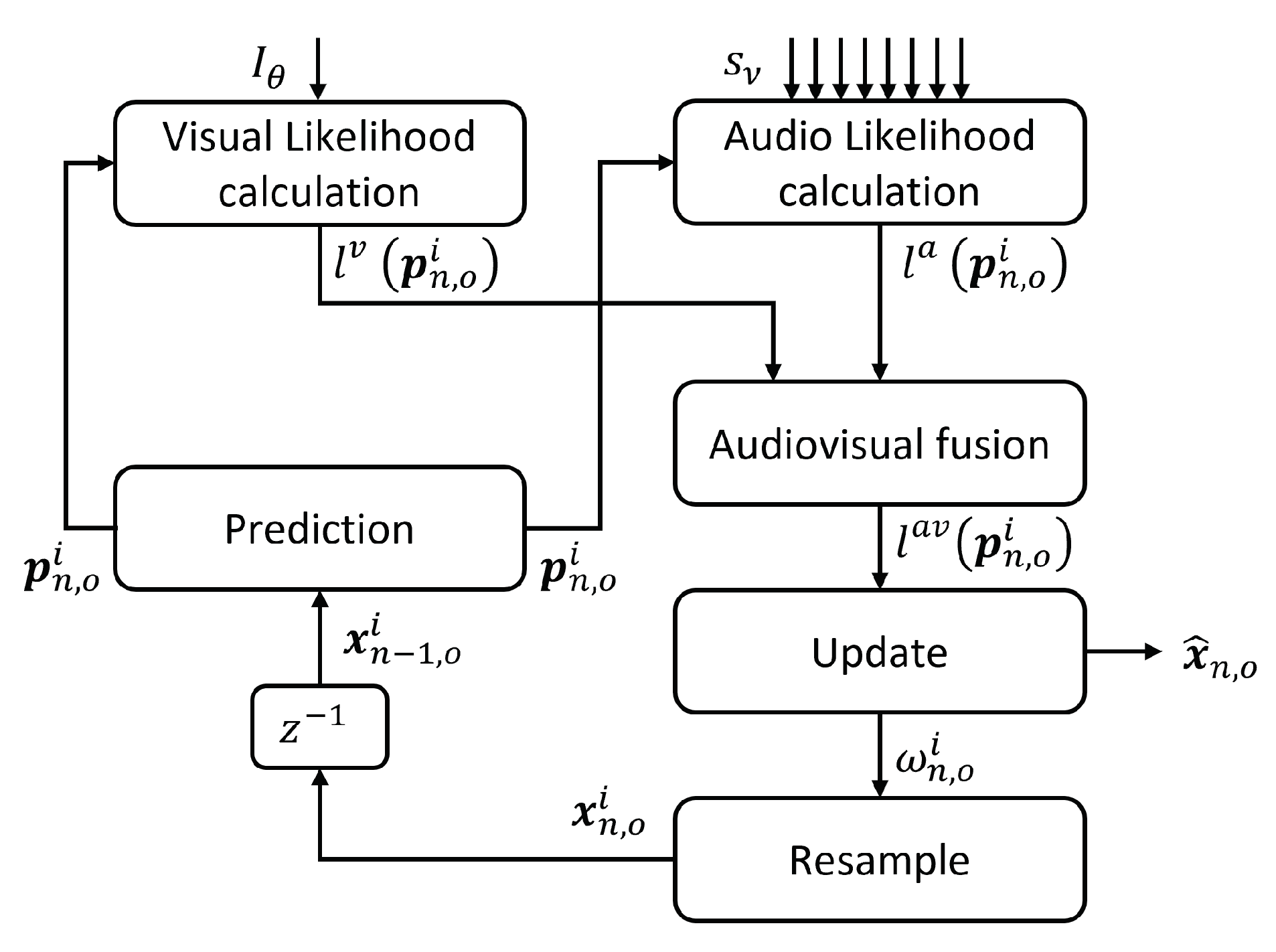
Figure 1.
Particle filter general scheme for multiple speakers audiovisual tracking.
Figure 1.
Particle filter general scheme for multiple speakers audiovisual tracking.
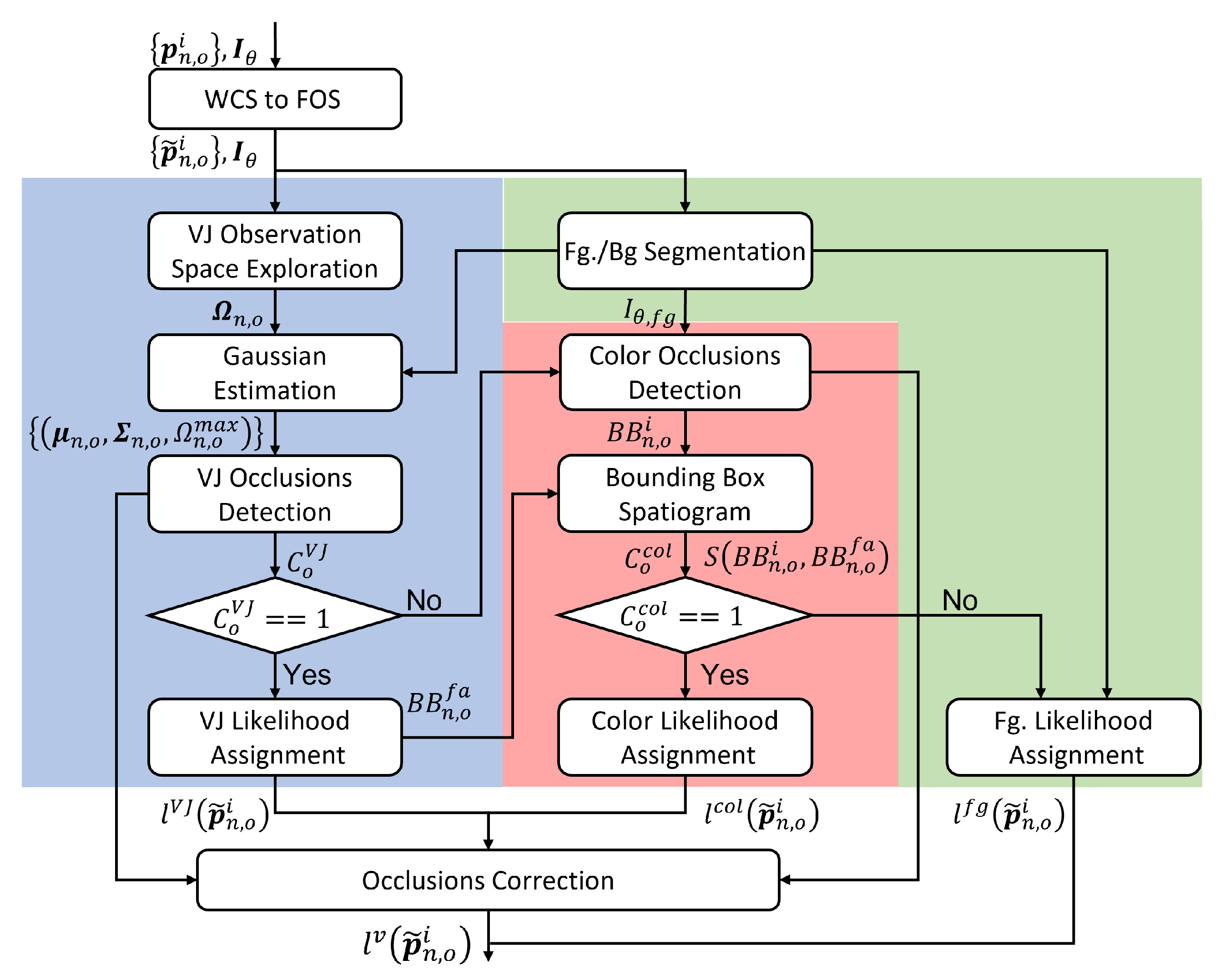
Figure 2.
Video observation model: VJ Likelihood (light blue) Color-based Likelihood (light red) and Fg. Likelihood (light green) blocks.
Figure 2.
Video observation model: VJ Likelihood (light blue) Color-based Likelihood (light red) and Fg. Likelihood (light green) blocks.
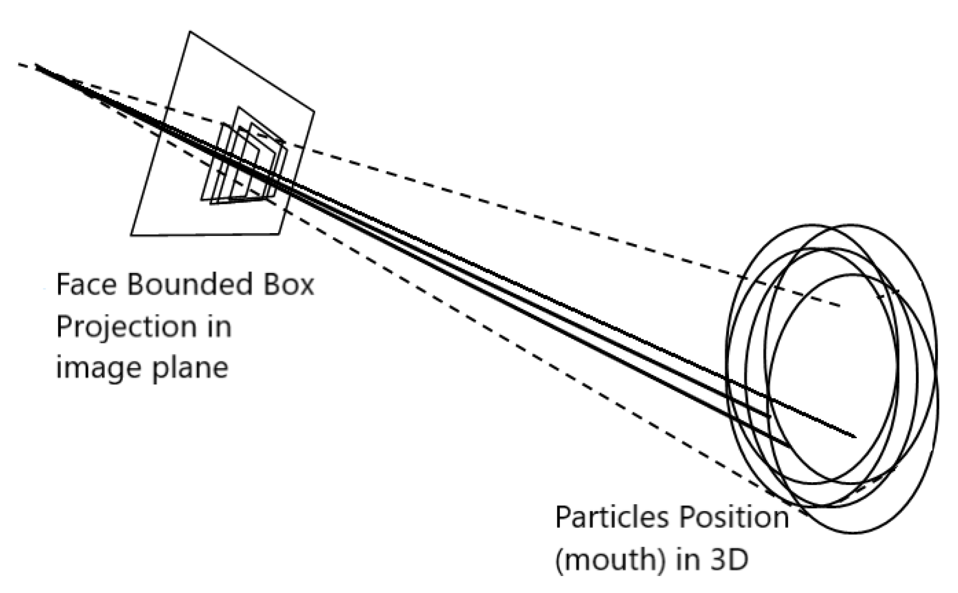
Figure 3.
Projections of each mouth hypothesis in the 3D WCS to its corresponding 2D BB in the FOS .
Figure 3.
Projections of each mouth hypothesis in the 3D WCS to its corresponding 2D BB in the FOS .
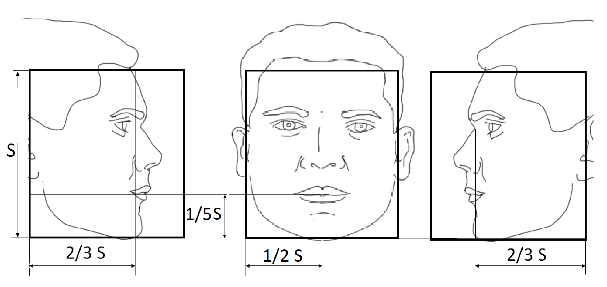
Figure 4.
Face templates for the right profile, frontal, and left profile poses.
Figure 4.
Face templates for the right profile, frontal, and left profile poses.
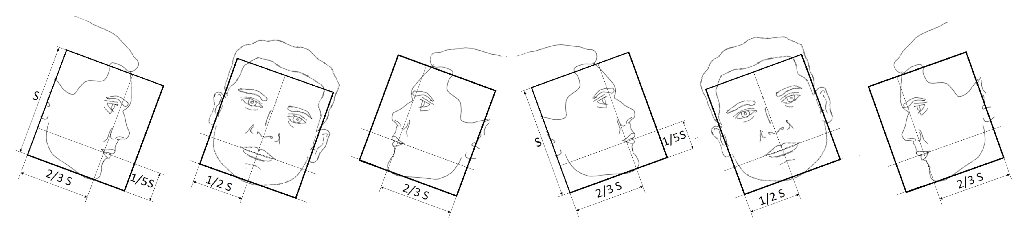
Figure 5.
Face templates with in-plane rotations with (counterclockwise, the three on the left, and clockwise the three on the right).
Figure 5.
Face templates with in-plane rotations with (counterclockwise, the three on the left, and clockwise the three on the right).
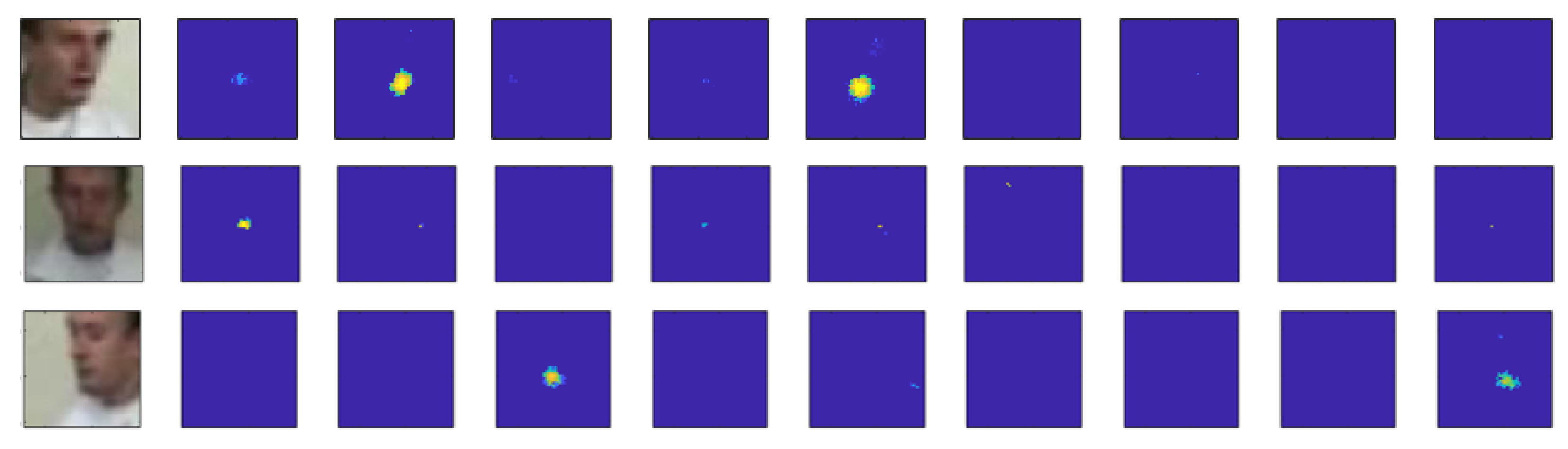
Figure 6.
Face likelihood model response for different poses: right at the top row, frontal at the middle row, and left at the bottom row. From left to right in each row: .
Figure 6.
Face likelihood model response for different poses: right at the top row, frontal at the middle row, and left at the bottom row. From left to right in each row: .
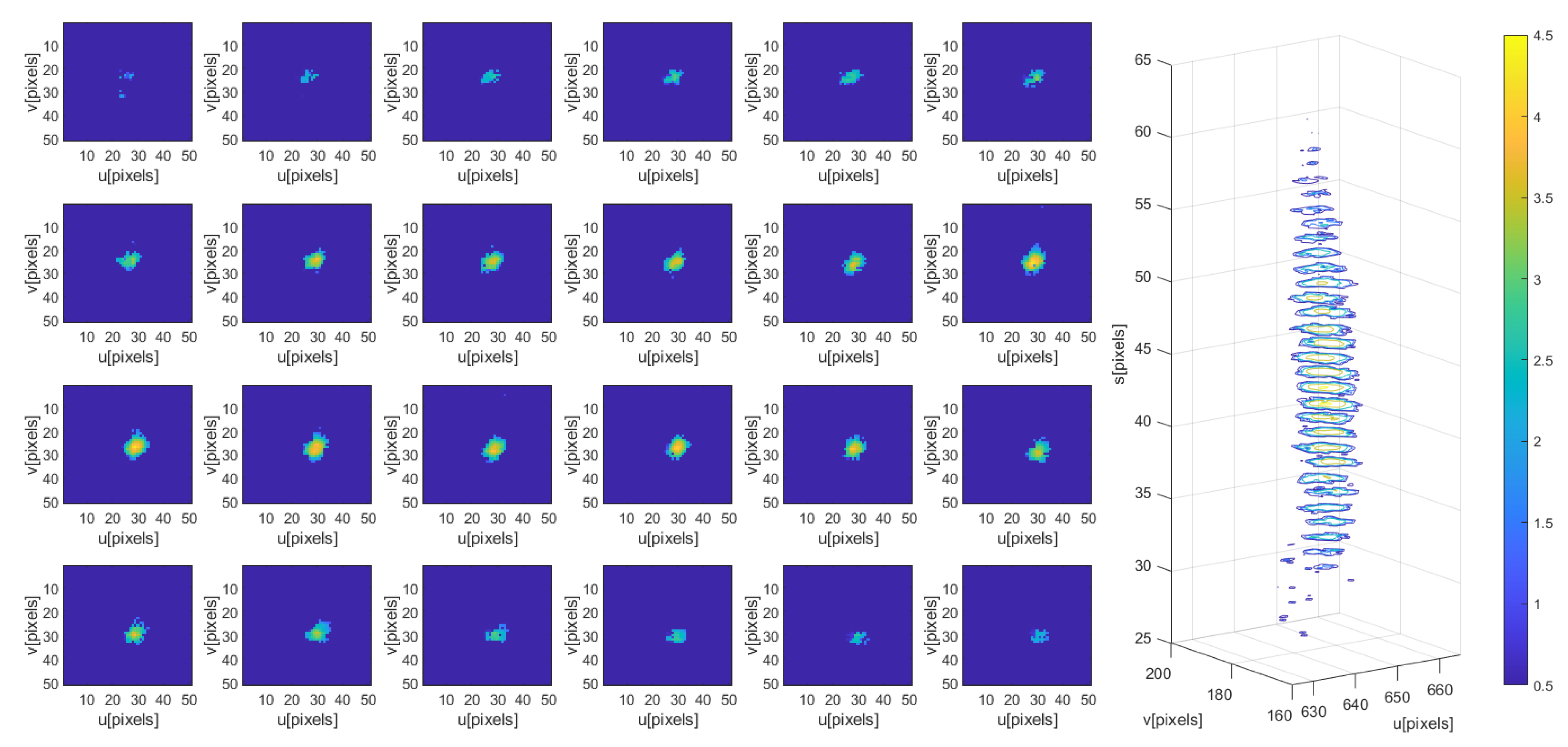
Figure 7.
Face likelihoods response at different 2D BB sizes () in pixels. (Left): likelihood maps. (Right): 3D plot of the likelihoods in the FOS .
Figure 7.
Face likelihoods response at different 2D BB sizes () in pixels. (Left): likelihood maps. (Right): 3D plot of the likelihoods in the FOS .
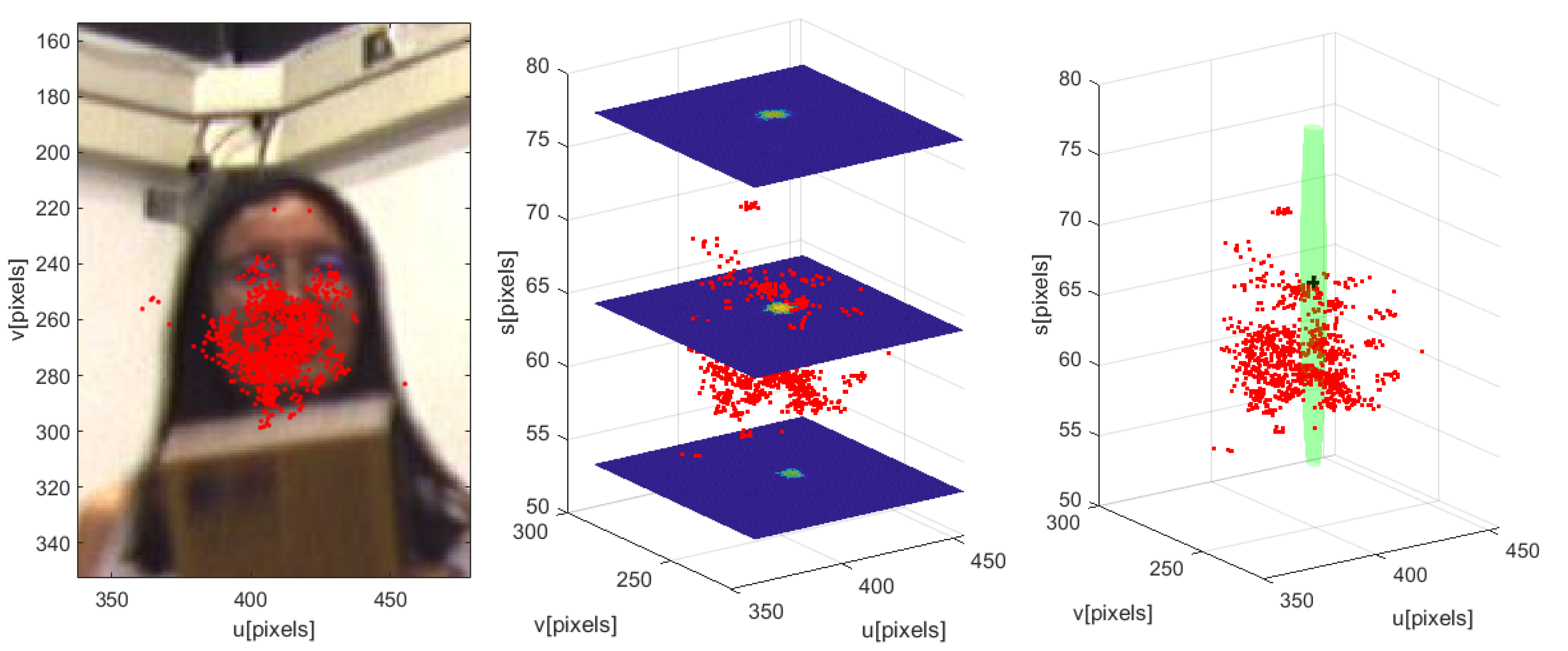
Figure 8.
VJ Likelihood Model: Predicted particles (red dots) projected on the image (left), the three slices in the S dimension (middle) with the particles (red dots), and the estimated Gaussian (green blob) along with particles (red dots) in the FOS (right).
Figure 8.
VJ Likelihood Model: Predicted particles (red dots) projected on the image (left), the three slices in the S dimension (middle) with the particles (red dots), and the estimated Gaussian (green blob) along with particles (red dots) in the FOS (right).
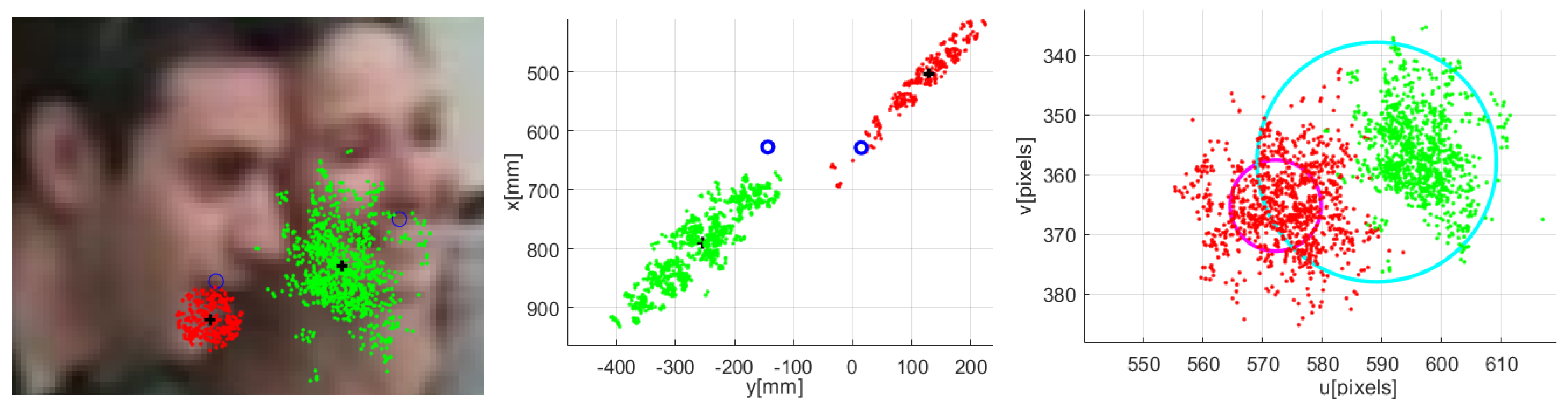
Figure 9.
Occlusion situation. Image with particles’ projection (left). Top view of 3D position-related particles (middle). The same with standard deviation circles (right). For target one the particles are in red color, and the standard deviation circle in magenta. For target two the particles are in green color, and the standard deviation circle in cyan.
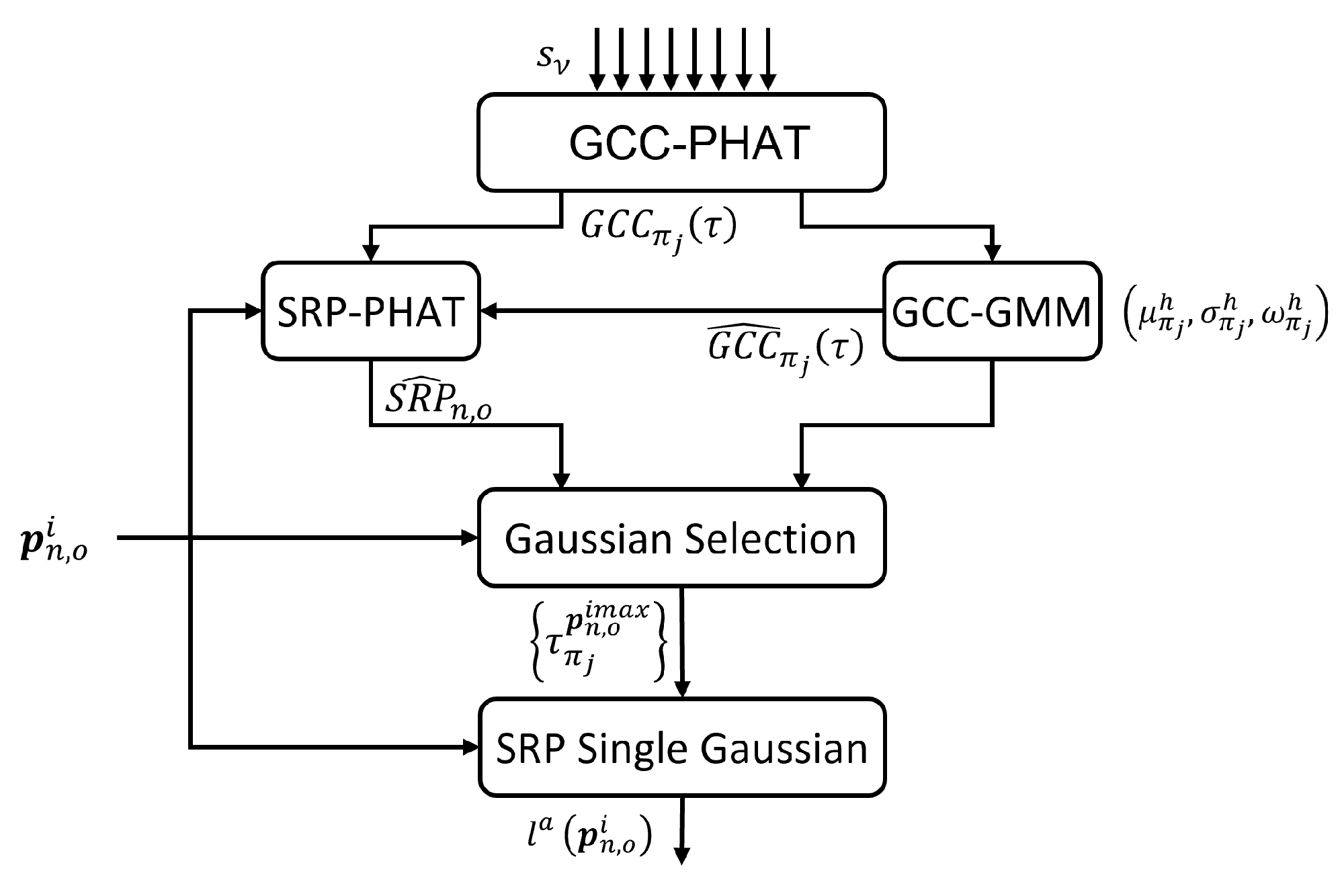
Figure 10.
General scheme of the audio likelihood model.
Figure 10.
General scheme of the audio likelihood model.
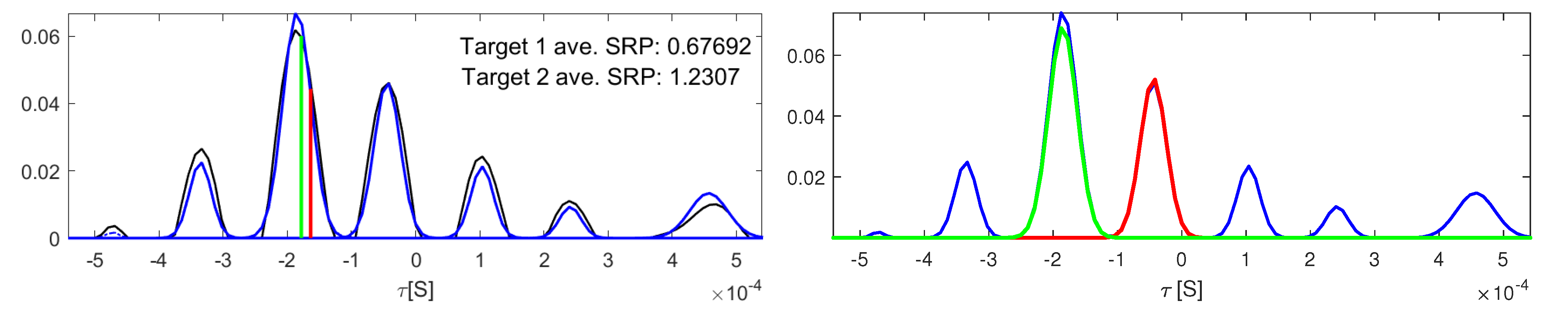
Figure 11.
Gaussian selection. In the left graphic: in black, and in blue. In the right graphic: selected Gaussians for target 1 (red) and target 2 (green). The GMM model was generated with .
Figure 11.
Gaussian selection. In the left graphic: in black, and in blue. In the right graphic: selected Gaussians for target 1 (red) and target 2 (green). The GMM model was generated with .
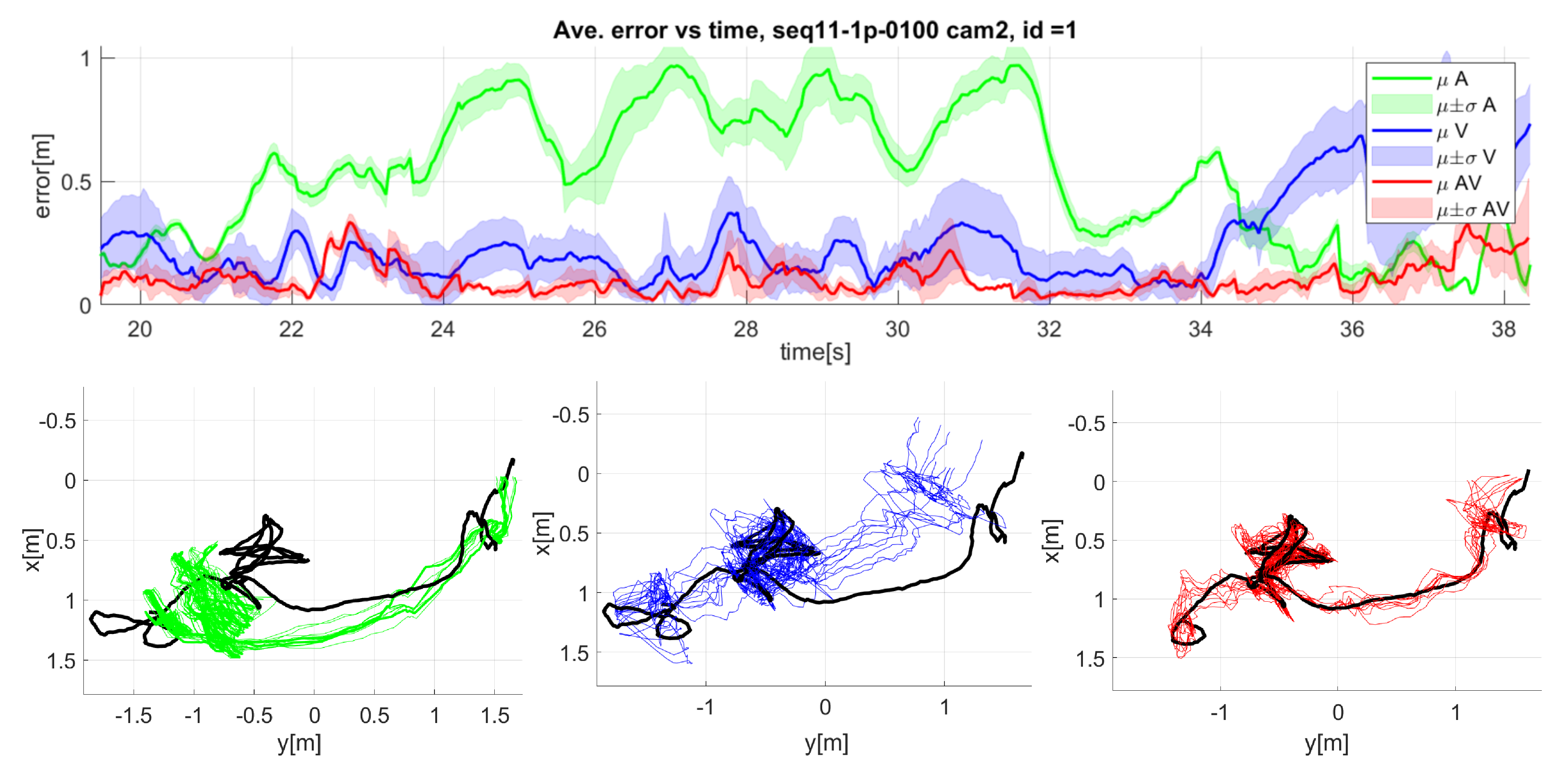
Figure 12.
Detailed results for seq11 camera 2: Mean and standard deviation of error over time (top graphic), and top view of the speaker trajectory (bottom graphics). Green: audio only, blue: video only, red: audiovisual, black: ground truth).
Figure 12.
Detailed results for seq11 camera 2: Mean and standard deviation of error over time (top graphic), and top view of the speaker trajectory (bottom graphics). Green: audio only, blue: video only, red: audiovisual, black: ground truth).
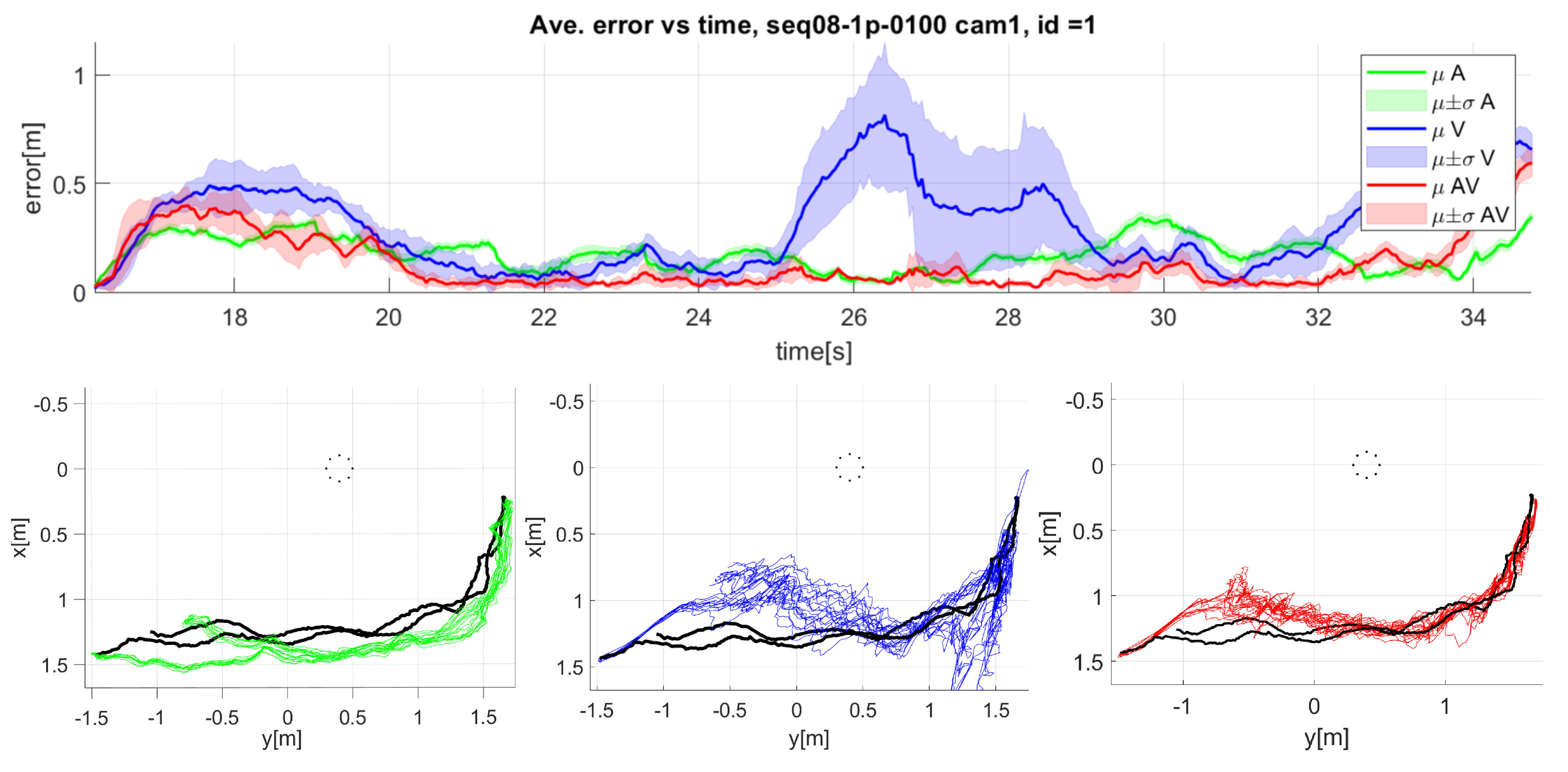
Figure 13.
Detailed results for seq08 camera 1: Mean and standard deviation of error over time (top graphic), and top view of the speaker trajectory (bottom graphics). Green: audio only, blue: video only, red: audiovisual, black: ground truth). The dotted circle represents the microphone array.
Figure 13.
Detailed results for seq08 camera 1: Mean and standard deviation of error over time (top graphic), and top view of the speaker trajectory (bottom graphics). Green: audio only, blue: video only, red: audiovisual, black: ground truth). The dotted circle represents the microphone array.
Figure 14.
Additional detailed results for sequences seq08 camera 3 and seq12 camera 1: Mean and standard deviation of error over time. Green: audio only, blue: video only, red: audiovisual, black: ground truth).
Figure 14.
Additional detailed results for sequences seq08 camera 3 and seq12 camera 1: Mean and standard deviation of error over time. Green: audio only, blue: video only, red: audiovisual, black: ground truth).
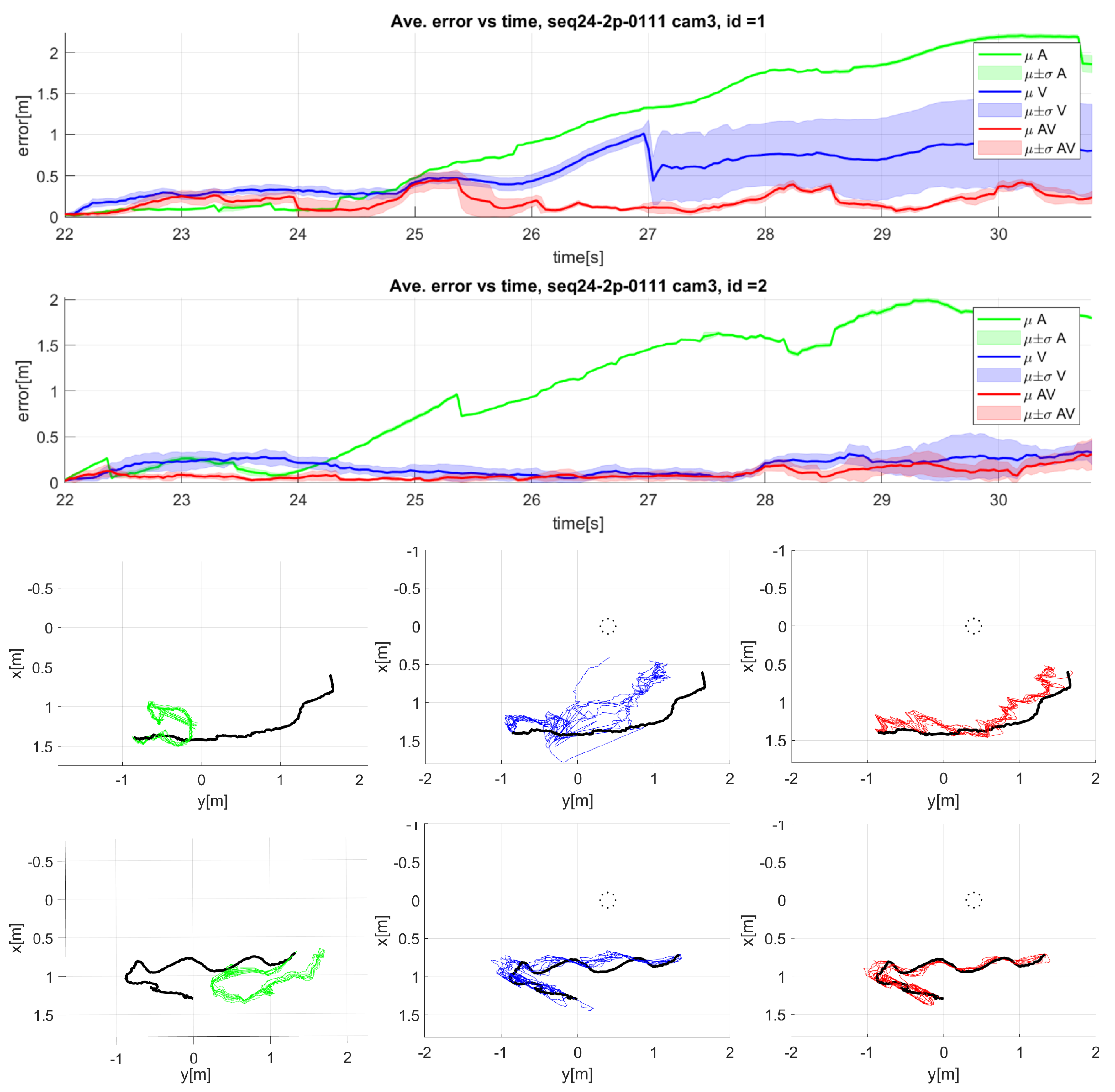
Figure 15.
Detailed results for sequence seq24 camera 3: Mean and standard deviation of error over time for the tracking of two speakers (top graphics), and top view of the 3D trajectories of both speakers (bottom graphics). Green: audio only, blue: video only, red: audiovisual, black: ground truth. Speaker one graphics are above those of speaker two. The dotted circle represents the microphone array.
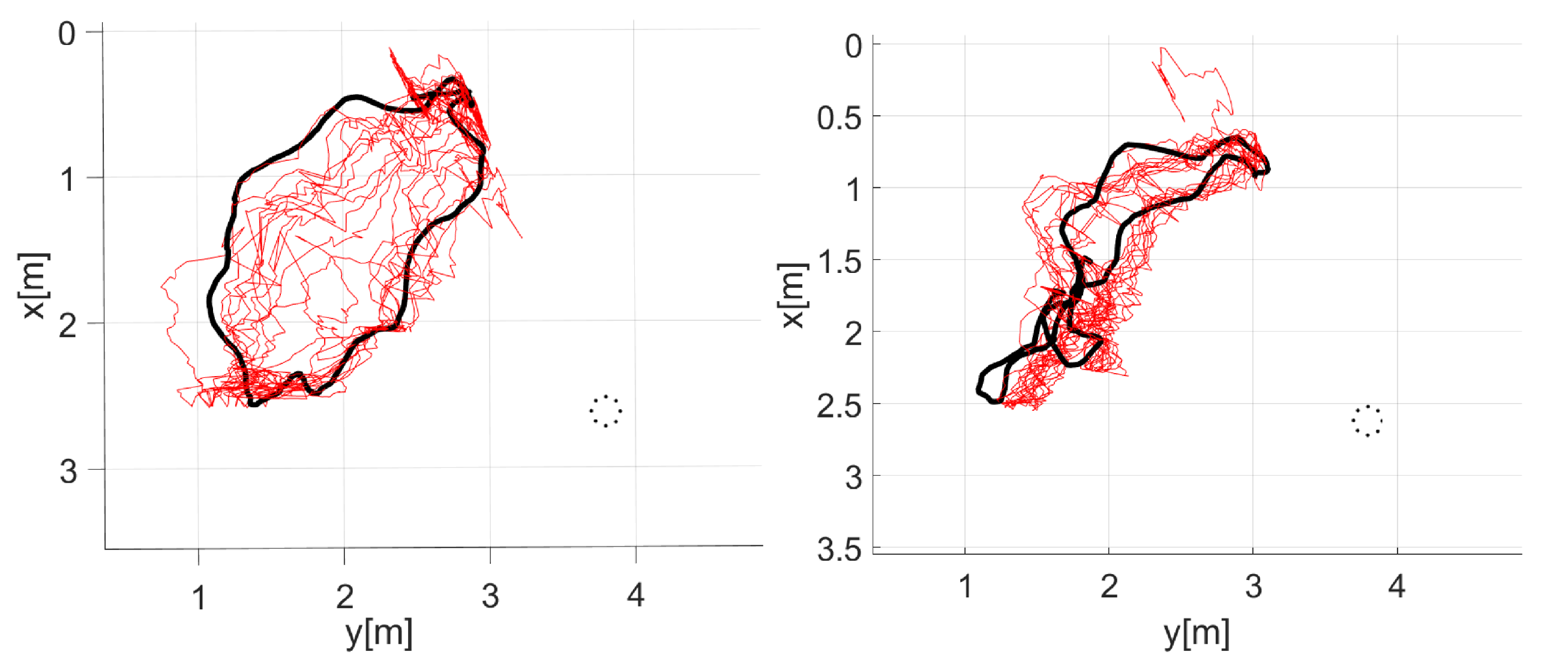
Figure 16.
Top view of the 3D trajectories for the two speakers in the seq22 camera 5 (red: audiovisual, black: ground truth). The dotted circle represents the microphone array.
Figure 16.
Top view of the 3D trajectories for the two speakers in the seq22 camera 5 (red: audiovisual, black: ground truth). The dotted circle represents the microphone array.
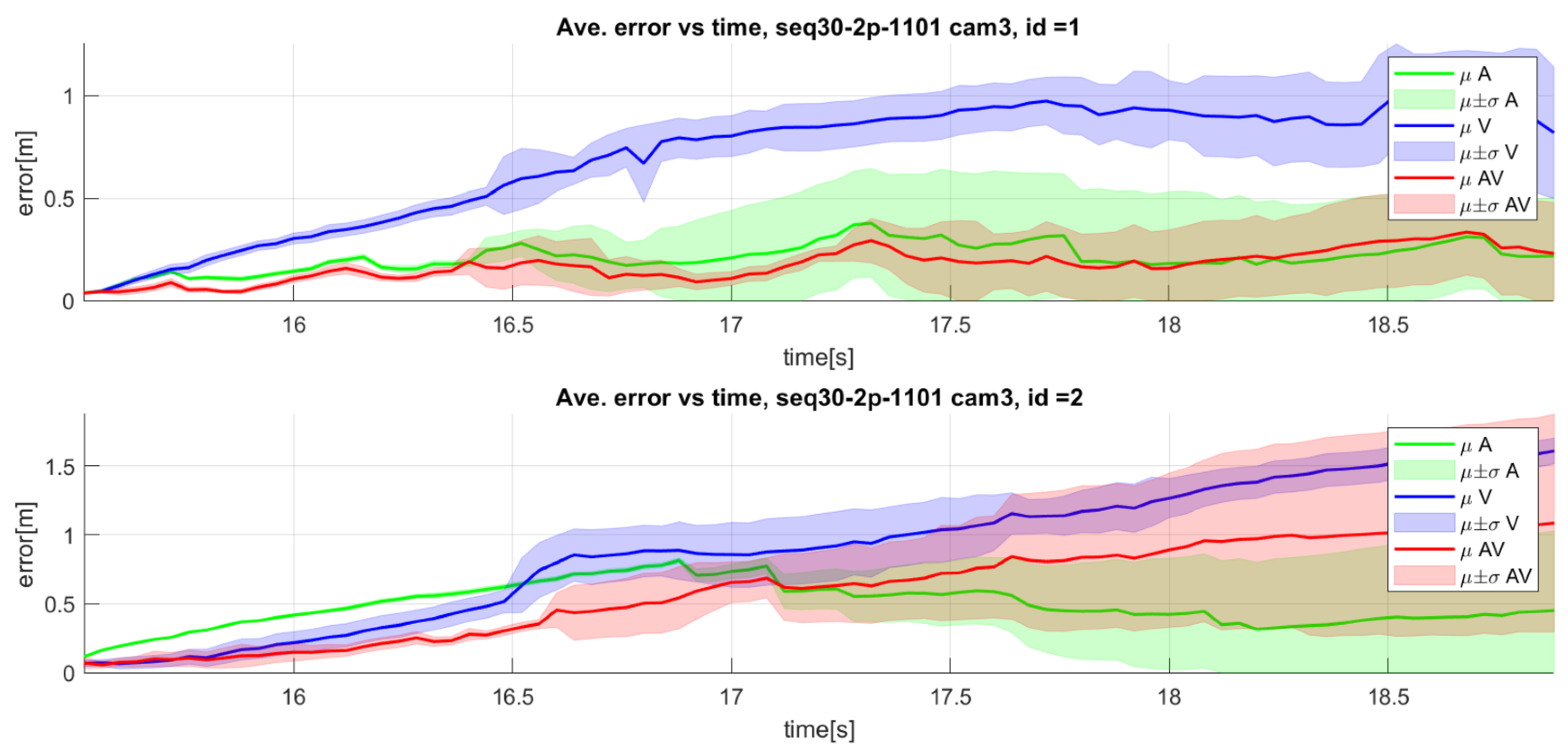
Figure 17.
Detailed results for sequence seq30 camera 3: Mean and standard deviation of error over time. Top: speaker 1; Bottom: speaker 2. Green: audio only, blue: video only, red: audiovisual, black: ground truth).
Figure 17.
Detailed results for sequence seq30 camera 3: Mean and standard deviation of error over time. Top: speaker 1; Bottom: speaker 2. Green: audio only, blue: video only, red: audiovisual, black: ground truth).
Table 1.
Brief descriptions of the sequences in the AV16.3 dataset.
Table 1.
Brief descriptions of the sequences in the AV16.3 dataset.
| Type | Sequence ID | Description | Time Length (MM:SS) |
|---|
| SOT | seq08 | Moving speaker facing the array, walking backward and forward once | 00:22.28 |
| SOT | seq11 | Moving speaker facing the array, doing random motions | 00:30.76 |
| SOT | seq12 | Moving speaker facing the array, doing random motions | 00:48.16 |
| | | Total SOT | 01:41.20 |
| MOT | seq18 | Two moving speakers facing the array, speaking continuously, growing closer to each other, then further apart twice, the first time seated and the second time standing | 00:57.00 |
| MOT | seq19 | Two standing speakers facing the array, speaking continuously, growing closer to each other, then further from each other | 00:22.8 |
| MOT | seq24 | Two moving speakers facing the array, speaking continuously, walking backward and forward, each speaker starting from the opposite side and occluding the other one once | 00:47.96 |
| MOT | seq25 | Two moving speakers greeting each other, discussing, then parting, without occluding each other | 00:55.72 |
| MOT | seq30 | Two moving speakers, both speaking continuously, walking backward and forward once, one behind the other at a constant distance | 00:22.04 |
| | | Total MOT | 03:56.28 |
| | | TOTAL ALL | 05:37.48 |
Table 2.
Brief descriptions of the sequences in the CAV3D dataset.
Table 2.
Brief descriptions of the sequences in the CAV3D dataset.
| Type | Sequence ID | Description | Time Length (MM:SS) |
|---|
| SOT | seq06 | Female moving along a reduced area inside the room. | 00:52.10 |
| SOT | seq07 | Male moving along a reduced area inside the room | 00:58.97 |
| SOT | seq08 | Male moving along a reduced area inside the room | 01:10.02 |
| SOT | seq09 | Male moving along a reduced area inside the room within noisy situations | 00:50.43 |
| SOT | seq10 | Male moving along a reduced area inside the room within noisy situations | 00:50.05 |
| SOT | seq11 | Male moving along a reduced area inside the room within clapping/noising and bending/sitting situations | 01:10.61 |
| SOT | seq12 | Male moving along a reduced area inside the room within clapping/noising and bending/sitting situations | 01:28.87 |
| SOT | seq13 | Male moving along the whole room | 01:24.22 |
| SOT | seq20 | Male moving along a reduced area inside the room | 00:46.46 |
| | | Total SOT | 9:31.73 |
| MOT | seq22 | A female and a male moving along the room simultaneously speaking | 00:39.55 |
| MOT | seq23 | A female and a male moving along the room simultaneously speaking | 01:04.04 |
| MOT | seq24 | A female and a male moving along the room simultaneously speaking | 01:09.46 |
| MOT | seq25 | Two females and a male moving along the room simultaneously speaking | 01:02.46 |
| MOT | seq26 | Two females and a male moving along the room simultaneously speaking | 00:36.48 |
| | | Total MOT | 04:31.99 |
| | | TOTAL ALL | 14:03.72 |
Table 3.
Performance scores of GAVT on AV16.3. Average TLR [%] and MAE in 2D [pixels] per modality (A: audio-only, V: video-only, and AV: audiovisual), and summary comparison (: improvement from A to AV, : improvement from V to AV). The best results across metrics are highlighted with a green background.
| | | GAVT on AV16.3 in 2D (A, V, AV and Comparison) |
|---|
| | | A | V | AV | | |
|---|
| SOT | TLR | 65.35 ± 3.50 | 6.42 ± 3.54 | 5.19 ± 2.55 | 92.1% | 19.2% |
| 37.09 ± 2.53 | 5.78 ± 2.11 | 5.12 ± 1.42 | 86.2% | 11.4% |
| 8.98 ± 0.41 | 3.35 ± 0.12 | 3.35 ± 0.10 | 62.6% | −0.1% |
| MOT | TLR | 74.56 ± 6.87 | 20.19 ± 7.49 | 9.55 ± 7.26 | 87.2% | 52.7% |
| 57.01 ± 12.12 | 14.29 ± 7.08 | 7.40 ± 5.46 | 87.0% | 48.2% |
| 8.39 ± 0.80 | 3.15 ± 0.33 | 3.27 ± 0.32 | 61.0% | −4.0% |
| Avg | TLR | 69.95 ± 5.18 | 13.31 ± 5.51 | 7.37 ± 4.91 | 89.5% | 44.6% |
| 47.05 ± 7.32 | 10.03 ± 4.60 | 6.26 ± 3.44 | 86.7% | 37.6% |
| 8.69 ± 0.60 | 3.25 ± 0.22 | 3.31 ± 0.21 | 61.9% | −2.0% |
Table 4.
Performance scores of GAVT on AV16.3. Average TLR [%] and MAE in 3D [m] per modality (A: audio-only, V: video-only, and AV: audiovisual), and summary comparison (: improvement from A to AV, : improvement from V to AV). The best results across metrics are highlighted with a green background.
| | | GAVT on AV16.3 in 3D (A, V, AV and Comparison) |
|---|
| | | A | V | AV | | |
|---|
| SOT | TLR | 43.80 ± 2.78 | 46.76 ± 6.14 | 12.05 ± 3.84 | 72.5% | 74.2% |
| 0.37 ± 0.02 | 0.33 ± 0.04 | 0.15 ± 0.01 | 59.4% | 54.6% |
| 0.17 ± 0.01 | 0.15 ± 0.01 | 0.10 ± 0.01 | 38.8% | 29.3% |
| MOT | TLR | 59.88 ± 9.07 | 46.15 ± 9.58 | 19.78 ± 11.0 | 67.0% | 57.1% |
| 0.68 ± 0.15 | 0.39 ± 0.09 | 0.21 ± 0.08 | 69.7% | 46.7% |
| 0.16 ± 0.02 | ;0.15 ± 0.02 | 0.11 ± 0.01 | 26.1% | 24.2% |
| Avg | TLR | 51.84 ± 5.93 | 46.46 ± 7.86 | 15.92 ± 7.43 | 69.3% | 65.7% |
| 0.52 ± 0.09 | 0.36 ± 0.06 | 0.18 ± 0.12 | 66.1% | 50.3% |
| 0.16 ± 0.01 | 0.15 ± 0.02 | 0.11 ± 0.01 | 32.7% | 26.7% |
Table 5.
Performance scores of AV3T and GAVT on AV16.3. Average TLR [%] and MAE in 2D [pixels] for the audio-only (A) and video-only (V) modalities, and summary improvements comparison of GAVT to AV3T (). The best results across metrics are highlighted with a green background.
Table 5.
Performance scores of AV3T and GAVT on AV16.3. Average TLR [%] and MAE in 2D [pixels] for the audio-only (A) and video-only (V) modalities, and summary improvements comparison of GAVT to AV3T (). The best results across metrics are highlighted with a green background.
| | | GAVT, AV3T and Comparison, on AV16.3 in 2D (A and V) |
|---|
| | | A | V |
|---|
| | | AV3T | GAVT | | AV3T | GAVT | |
|---|
| SOT | TLR | 48.10 ± 6.00 | 65.35 ± 3.50 | −36% | 9.00 ± 1.90 | 6.42 ± 3.54 | 29% |
| 24.10 ± 5.70 | 37.09 ± 2.53 | −54% | 8.20 ± 1.10 | 5.78 ± 2.11 | 30% |
| 7.60 ± 0.50 | 8.98 ± 0.41 | −18% | 5.30 ± 0.10 | 3.35 ± 0.12 | 37% |
| MOT | TLR | 56.60 ± 9.40 | 74.56 ± 6.87 | −32% | 15.50 ± 9.00 | 20.19 ± 7.49 | −30% |
| 38.40 ± 9.20 | 57.01 ± 12.1 | −48% | 17.90 ± 8.80 | 14.29 ± 7.08 | 20% |
| 7.70 ± 0.90 | 8.39 ± 0.80 | −9% | 5.10 ± 0.40 | 3.15 ± 0.33 | 38% |
| Avg | TLR | 52.35 ± 7.70 | 69.95 ± 5.18 | −34% | 12.25 ± 5.45 | 13.31 ± 5.51 | −9% |
| 31.25 ± 7.45 | 47.05 ± 7.32 | −51% | 13.05 ± 4.95 | 10.03 ± 4.60 | 23% |
| 7.65 ± 0.70 | 8.69 ± 0.60 | −14% | 5.20 ± 0.25 | 3.25 ± 0.22 | 38% |
Table 6.
Performance scores of AV3T and GAVT on AV16.3. Average TLR [%] and MAE in 3D [m] for the audio-only (A) and video-only (V) modalities, and summary improvements comparison of GAVT to AV3T (). The best results across metrics are highlighted with a green background.
Table 6.
Performance scores of AV3T and GAVT on AV16.3. Average TLR [%] and MAE in 3D [m] for the audio-only (A) and video-only (V) modalities, and summary improvements comparison of GAVT to AV3T (). The best results across metrics are highlighted with a green background.
| | | GAVT, AV3T and Comparison, on AV16.3 in 3D (A and V) |
|---|
| | | A | V |
|---|
| | | AV3T | GAVT | | AV3T | GAVT | |
|---|
| SOT | TLR | 34.90 ± 8.90 | 43.80 ± 2.78 | −26% | 52.70 ± 5.50 | 46.76 ± 6.14 | 11% |
| 0.28 ± 0.01 | 0.37 ± 0.02 | −30% | 0.41 ± 0.01 | 0.33 ± 0.04 | 20% |
| 0.15 ± 0.01 | 0.17 ± 0.01 | −14% | 0.16 ± 0.10 | 0.15 ± 0.01 | 8% |
| MOT | TLR | 44.90 ± 1.20 | 59.88 ± 9.07 | −33% | 56.30 ± 9.80 | 46.15 ± 9.58 | 18% |
| 0.48 ± 0.12 | 0.68 ± 0.15 | −42% | 0.52 ± 0.11 | 0.39 ± 0.09 | 26% |
| 0.15 ± 0.02 | 0.16 ± 0.02 | −4% | 0.15 ± 0.02 | 0.15 ± 0.02 | −1% |
| Avg | TLR | 39.90 ± 5.05 | 51.84 ± 5.93 | −30% | 54.50 ± 7.65 | 46.46 ± 7.86 | 15% |
| 0.38 ± 0.06 | 0.52 ± 0.09 | −38% | 0.47 ± 0.06 | 0.36 ± 0.06 | 23% |
| 0.15 ± 0.02 | 0.16 ± 0.01 | 9% | 0.16 ± 0.15 | 0.15 ± 0.02 | 3% |
Table 7.
Performance scores of AV3T and GAVT on AV16.3. Average TLR [%] and MAE in 2D [pixels] for the AV modality, and summary improvements comparison of GAVT to AV3T (). The best results across metrics are highlighted with a green background.
Table 7.
Performance scores of AV3T and GAVT on AV16.3. Average TLR [%] and MAE in 2D [pixels] for the AV modality, and summary improvements comparison of GAVT to AV3T (). The best results across metrics are highlighted with a green background.
| | | GAVT, AV3T and Comparison (AV), on AV16.3 in 2D |
|---|
| | | AV3T | GAVT | |
|---|
| SOT | TLR | 8.50 ± 3.60 | 5.19 ± 2.55 | 38.9% |
| 16.50 ± 8.60 | 5.12 ± 1.42 | 69.0% |
| 12.20 ± 0.30 | 3.35 ± 0.10 | 72.5% |
| MOT | TLR | 11.20 ± 5.90 | 9.55 ± 7.26 | 14.7% |
| 24.80 ± 23.7 | 7.40 ± 5.46 | 70.2% |
| 10.10 ± 0.60 | 3.27 ± 0.32 | 67.6% |
| Avg | TLR | 9.85 ± 4.75 | 7.37 ± 4.91 | 25.2% |
| 20.65 ± 16.1 | 6.26 ± 3.44 | 69.7% |
| 11.15 ± 0.45 | 3.31 ± 0.21 | 70.3% |
Table 8.
Performance scores of AV3T and GAVT on AV16.3. Average TLR [%] and MAE in 3D [m] for the AV modality, and summary improvements comparison of GAVT to AV3T (). The best results across metrics are highlighted with a green background.
Table 8.
Performance scores of AV3T and GAVT on AV16.3. Average TLR [%] and MAE in 3D [m] for the AV modality, and summary improvements comparison of GAVT to AV3T (). The best results across metrics are highlighted with a green background.
| | | GAVT, AV3T and Comparison (AV), on AV16.3 in 3D |
|---|
| | | AV3T | GAVT | |
|---|
| SOT | TLR | 13.30 ± 4.30 | 12.05 ± 3.84 | 9.4% |
| 0.16 ± 0.20 | 0.15 ± 0.15 | 7.4% |
| 0.11 ± 0.10 | 0.10 ± 0.01 | 5.1% |
| MOT | TLR | 15.80 ± 8.90 | 19.78 ± 11.0 | −25.2% |
| 0.21 ± 0.07 | 0.21 ± 0.08 | 1.8% |
| 0.11 ± 0.01 | 0.11 ± 0.01 | −4.4% |
| Avg | TLR | 14.55 ± 6.60 | 15.92 ± 7.43 | −9.4% |
| 0.19 ± 0.14 | 0.18 ± 0.12 | 4.2% |
| 0.11 ± 0.06 | 0.11 ± 0.01 | 0.3% |
Table 9.
Performance scores of AV3T and GAVT on CAV3D. Average TLR [%] and MAE in 2D [pixels] for the AV modality, and summary improvements comparison of GAVT to AV3T (). The best results across metrics are highlighted with a green background.
Table 9.
Performance scores of AV3T and GAVT on CAV3D. Average TLR [%] and MAE in 2D [pixels] for the AV modality, and summary improvements comparison of GAVT to AV3T (). The best results across metrics are highlighted with a green background.
| | | GAVT, AV3T and Comparison (AV), on CAV3D in 2D |
|---|
| | | AV3T | GAVT | |
|---|
| SOT | TLR | 7.00 ± 3.60 | 13.93 ± 5.41 | −99.0% |
| 16.50 ± 8.60 | 26.76 ± 10.8 | −62.2% |
| 12.20 ± 0.30 | 8.69 ± 0.49 | 28.7% |
| MOT | TLR | 11.20 ± 5.90 | 21.01 ± 14.7 | −87.6% |
| 24.80 ± 23.7 | 13.47 ± 10.4 | 45.7% |
| 10.1 ± 0.60 | 9.55 ± 0.18 | 5.4% |
| Avg | TLR | 9.10 ± 4.75 | 17.47 ± 10.1 | −92.0% |
| 20.65 ± 16.1 | 20.11 ± 10.6 | 2.6% |
| 11.15 ± 0.45 | 9.12 ± 0.33 | 18.2% |
Table 10.
Performance scores of AV3T and GAVT on CAV3D. Average TLR [%] and MAE in 3D [m] for the AV modality, and summary improvements comparison of GAVT to AV3T (). The best results across metrics are highlighted with a green background.
Table 10.
Performance scores of AV3T and GAVT on CAV3D. Average TLR [%] and MAE in 3D [m] for the AV modality, and summary improvements comparison of GAVT to AV3T (). The best results across metrics are highlighted with a green background.
| | | GAVT, AV3T and Comparison (AV), on CAV3D in 3D |
|---|
| | | AV3T | GAVT | |
|---|
| SOT | TLR | 31.80 ± 3.50 | 30.07 ± 4.14 | 5.4% |
| 0.30 ± 0.05 | 0.29 ± 0.04 | 2.1% |
| 0.16 ± 0.01 | 0.13 ± 0.01 | 21.8% |
| MOT | TLR | 35.70 ± 6.60 | 32.01 ± 4.13 | 10.3% |
| 0.43 ± 0.21 | 0.35 ± 0.08 | 18.1% |
| 0.15 ± 0.01 | 0.13 ± 0.01 | 13.7% |
| Avg | TLR | 33.75 ± 5.05 | 31.04 ± 4.14 | 8.0% |
| 0.37 ± 0.13 | 0.32 ± 0.06 | 11.5% |
| 0.16 ± 0.01 | 0.13 ± 0.01 | 17.9% |


