Abstract
The Iterative Closest Point (ICP) is a matching technique used to determine the transformation matrix that best minimizes the distance between two point clouds. Although mostly used for 2D and 3D surface reconstruction, this technique is also widely used for mobile robot self-localization by means of matching partial information provided by an onboard LIDAR scanner with a known map of the facility. Once the estimated position of the robot is obtained, the scans gathered by the LIDAR can be analyzed to locate possible obstacles obstructing the planned trajectory of the mobile robot. This work proposes to speed up the obstacle detection process by directly monitoring outliers (discrepant points between the LIDAR scans and the full map) spotted after ICP matching instead of spending time performing an isolated task to re-analyze the LIDAR scans to detect those discrepancies. In this work, a computationally optimized ICP implementation has been adapted to return the list of outliers along with other matching metrics, computed in an optimal way by taking advantage of the parameters already calculated in order to perform the ICP matching. The evaluation of this adapted ICP implementation in a real mobile robot application has shown that the time required to perform self-localization and obstacle detection has been reduced by 36.7% when obstacle detection is performed simultaneously with the ICP matching instead of implementing a redundant procedure for obstacle detection. The adapted ICP implementation is provided in the SLAMICP library.
1. Introduction
The most important capabilities expected of a mobile robot are the ability to locate its position, follow a planned path, and detect and avoid unexpected obstacles appearing in the vicinity of the robot. Odometry is a direct computation method that provides a periodic update of the location of a mobile robot [1] based on the information of the angular velocity of the wheels and a precise estimation of the inverse kinematic matrix of the mobile robot [2]. However, this estimation method is prone to errors due to the structural uncertainties originated during the manufacturing process, which can lead to systematic odometry errors [3,4]. One example of such parameters affecting the inverse kinematics is the effective radius of the wheels [5], which may change depending on the air pressure in the wheel chamber (in the case of using wheels with an air chamber), the hardness of the rubber that is in contact with the ground, and the relative weight distribution of the robot. The effects of such uncertainties and some methods to calibrate the Inverse kinematic matrix have been deeply analyzed by the scientific community [6,7,8,9,10,11,12]. When the kinematics are calibrated, the relative displacement of a mobile robot can be estimated by multiplying the current estimation of the angular velocity of its wheels by its inverse kinematic matrix and the elapsed time since the last estimation. This relative cumulated displacement updates the position and orientation of the mobile robot and defines its trajectory.
Unavoidable external factors such as traction loss (wheel slippage or skidding) or the accuracy of the encoders used to monitor the angular velocity of the wheels [13,14,15,16] can heavily undermine the accuracy of this relative odometry. Alternatively, vision-based [17,18] and light detection and ranging (LIDAR) [19,20] are alternative computational methods that can be used to provide a periodic estimation of the absolute position of a mobile robot when wheel-speed-based odometry becomes too unreliable. In general, LIDAR odometry requires matching the point cloud generated by onboard 2D or 3D LIDARs with a reference point cloud that describes the scenario being explored, a procedure that is also known as geometric registration [21]. LIDAR-based odometry methods can be divided into three categories: based on the Iterative Closest Point (ICP) algorithm [22,23,24,25,26,27,28] introduced by Chen et al. [21] and Besl et al. [29], based on the detection of features [30,31,32,33,34,35], and based on deep learning methods [36].
ICP-based methods are based on the direct matching of the point cloud provided by a LIDAR sensor with a reference point cloud [37]. This approach tries to find the transformation matrix [21,29] that best minimizes the distance between active points of the LIDAR point cloud and the reference point cloud. Usually, the LIDAR point cloud is provided by a 2D or 3D scanner located onboard the mobile robot [38], and the reference point cloud contains a 2D or 3D representation of the area being explored. The ICP algorithm iteratively estimates the transformation matrix that minimizes an error metric, which is usually the sum of squared differences between the coordinates of the point clouds to be matched. For example, Bhandari et al. [39] proposed using the ICP algorithm to track the position of an object with a known geometry in a six degrees of freedom (DOF) registration problem from point cloud measurements.
Feature-based methods are centered on the extraction of recognizable geometric features from point clouds such as line segments, planes, and features in order to efficiently determine the existing correspondences [30,32,34,35,40]. This approach has the advantage of speeding up the iterative matching process [41], as a large point cloud can be simplified into a small number of characteristic geometric features, representing a significant reduction in the amount of information that must be handled during the matching process. Zang et al. [30] proposed the first feature-based matching method for fast, accurate LIDAR odometry and mapping (LOAM) using real-time LIDAR data. Qin et al. [35] further speeded up LOAM by relying only on good features to perform the feature selection.
Deep learning methods use artificial neural networks to operate with large amounts of data [36]. Deep learning methods have been applied to perform feature matching [42,43] and to estimate odometry using the point cloud as input data [44,45,46,47,48]. For example, Jung et al. [49] proposed a deep learning-based LIDAR odometry estimation method using a long-term recurrent convolutional network (LRCN), using point clouds as the input data for the deep learning algorithm. This approach processes spatial and temporal information at once by using a convolutional neural network (CNN) and a long-short-term memory (LSTM) artificial neural network. Their proposal was suitable for accurately estimating the position of a six-DOF robot from the point cloud information.
This work is based on the use of the ICP algorithm to find the best transformation matrix to minimize the distance between the point cloud provided by the 2D LIDAR of an autonomous mobile robot and a reference point cloud that contains a 2D map describing the layout of the floor on which the robot is navigating. As stated previously, in cases where the map of the area is not available, the previous point cloud gathered by the mobile robot can be used as a reference, allowing the determination of the position difference between the coordinates at which the robot took the first scan and its current position. Then, the relative transformation matrix found by the ICP matching algorithm (which includes rotation and translation transformations) can be used to combine both point clouds into a single one in order to create a partial map description of the area in which the robot is navigating. This procedure can be repeated until the entire navigable area has been scanned, allowing the creation of a complete map of the application scenario [50]. The combined capability of providing simultaneous localization and mapping (SLAM [51]) is a feature widely implemented in mobile robots [52,53].
In general, the point cloud gathered from a 2D or 3D LIDAR sensor depicts a small area around the robot, but the reference point cloud describing or mapping a complete scenario tends to be very large. In such conditions, the main known drawback of using the ICP algorithm is the time required to iteratively find the best match between the point cloud gathered from a LIDAR and the map [54]. The optimized implementation of ICP matching has been addressed using different approaches [37]. For example, voxelization is a technique that divides the points contained in point clouds into small groups (or voxels) according to the normal distribution of each sub-point cloud. Voxelization is a simple yet effective approach to speeding up the ICP algorithm [55,56], although the reduction in the number of points also reduces the accuracy of the ICP matching [56]. The use of hardware acceleration is another effective approach to significantly reducing the execution time required by the ICP algorithm to find a suitable matching transformation [57].
Finally, the scan information provided by the LIDARs embedded in mobile robots is usually analyzed to detect and localize obstacles in the trajectory of the robot and, if required, update the map or implement specific obstacle avoidance procedures [58,59,60]. The exhaustive detection of discrepancies between the current LIDAR scan and the reference map is usually performed after ICP matching, as it requires the application of rotation and translation to the LIDAR scan points in order to fit them into the coordinates of the map. However, a closer look into the ICP matching algorithm reveals that this iterative procedure computes several variables that are relevant in the process of detecting discrepancies with the reference map. Therefore, the step of detecting the discrepant points again after the ICP matching could be optimized by taking advantage of the analysis already conducted as part of the ICP algorithm execution. Unfortunately, most ICP implementations available [22,23,24,25,26,27,28] discard all the internal variables after finishing the iterative process. The main goal of this work is to fuse the tasks of obstacle detection and mobile robot self-localization as a way to reduce the computational time required to detect obstacles around the mobile robot. This goal can be achieved by reusing the variables already computed during the detection of outliers as part of the ICP matching process.
New Contribution
This work proposes speeding up the obstacle detection process in mobile robot navigation by directly monitoring outliers spotted after Iterative Closest Point (ICP) matching. In this context, the outliers are the discrepant points found after matching the point clouds provided in a partial LIDAR scan gathered by the mobile robot and a full facility map. Monitoring the outliers spotted after the ICP matching avoids the need to re-analyze the LIDAR scans to detect obstacles (discrepancies) with the facility map in mobile robot navigation. As a result, the time required to perform self-localization and obstacle detection in a real mobile robot application can be significantly improved. This work also presents the ICP implementation developed to return the list of outliers along with other relevant matching parameters and metrics. This optimized ICP-based obstacle detection agent designed to retrieve the list of outliers while simultaneously performing localization and mapping is freely available as SLAMICP [61]. This new ICP implementation is based on the LIBrary for Iterative Closest Point fitting (LIBICP [62]), developed by Geiger et al. [63] to analyze the KITTI Dataset [64,65]. Both ICP libraries are available under the GNU public license [66] and include MATLAB wrappers for fast prototype implementation and evaluation.
The paper Is structured as follows. Section 2 describes the materials and methods. In Section 3, the new adaptations implemented in the SLAMICP [61] library are presented in a detailed manner. Section 4 presents the experimental results obtained in an application with a real autonomous mobile robot. Final remarks are given in Section 5.
2. Materials and Methods
The materials and methods used in this work are: the mobile robot used in the validation experiments, the area in which the validation experiments have been carried out, the vanilla ICP algorithm, the reference computationally optimized LIBICP [62] library implementing the ICP algorithm, the reference trajectory defined to implement the validation experiments, the reference obstacles used, and the performance metric used to assess the improvement in execution time of the procedure used to detect obstacles during mobile robot navigation.
2.1. Mobile Robot
The mobile robot used in this work is the APR-02, the second prototype of the APR robot series, developed by the Robotics Research Laboratory of the University of Lleida (Lleida, Spain) [67], which is shown in Figure 1. This mobile robot has been used to validate practical applications such as early gas leak detection [68] and enhance the sense of attention [69]. The robot has also been used as a platform test bench for alternative designs of omnidirectional wheels [70] and PID wheel control tuning [71]. The mobile robot embeds different sensors and actuators [67]: one 2D Hokuyo UTM-30 LIDAR for self-localization, one panoramic RGB camera on top of its head, three RGB-D Creative Senz3D cameras used for human interaction and ground validation, 8 fixed infrared distance detectors are used to provide interaction when the LIDAR is powered off; 16 passive infrared detectors are used to detect human activity and occupancy; 8 digital servomotors are used in the arms for gesticulation; redundant ambient sensors are used; and one touch screen is used to display an animated face and other interaction information.
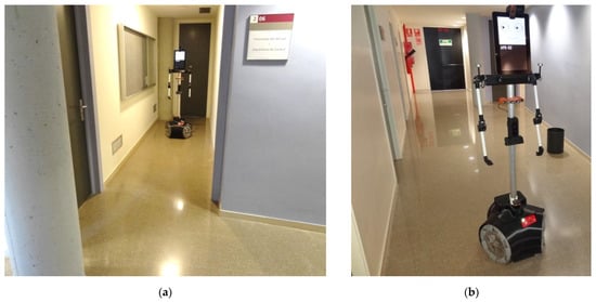
Figure 1.
Two pictures of the mobile robot APR-02 while conducting the validation experiments: (a) starting position of the experiment; and (b) final position of the experiment.
2.2. Experimentation Area
The experimentation area in which the experiments have been carried out is located in the Polytechnic School of the University of Lleida, Spain. The validation experiments have been conducted at the end of the corridor on the second floor (see Figure 1a), which has a small lateral junction contiguous to the central corridor (see Figure 1b). This area was considered ideal for experimenting with obstacle detection because the intersection of the two corridors allows us to recreate a scenario where an obstacle suddenly appears near the path of the robot. Figure 1a shows the mobile robot ARP-02 located in a position that will be the starting point of a reference trajectory implemented in this work, and Figure 1b also shows the mobile robot in the middle of the corridor, near the ending position of the reference trajectory. Figure 1b also shows a wastebasket randomly placed in the corridor as an example of an obstacle appearing in the trajectory of the mobile robot.
2.3. Vanilla ICP Algorithm
The vanilla Iterative Closet Point (ICP) algorithm iteratively minimizes point-to-point distances between point clouds [29]. Given a point cloud with points describing a 2D or 3D map of the floor of a building.
and a partial point cloud with points describing partial spatial information, for example, obtained with a 2D LIDAR or 3D LIDAR:
The ICP matching algorithm iteratively searches for the best match between the partial point cloud and the map of the scenario being explored. In each iteration, the ICP algorithm selects the closest points as correspondences and calculates the transformation that minimizes the following equation:
where are the weights of a point-to-point match, which are assigned as if is the closest point to and if the distance between and is greater than a predetermined outlier threshold distance. Then, the outliers are the points in that cannot be matched to any point in .
Figure 2 shows the schematic representation of point clouds with no measurement errors, so the plot of the individual points that define the location of the walls looks like straight lines. Figure 2a represents an ideal reference or map point cloud obtained by the 2D LIDAR of a mobile robot placed in a starting position. The assumption is that a complete map of the environment is not available. Figure 2b represents an ideal partial point cloud obtained after the robot has moved. These 2D point clouds, and , can be expressed as:
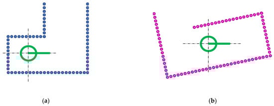
Figure 2.
Schematic representation of the 2D point clouds gathered from a mobile robot (green circle): (a) reference partial point cloud (blue dots) obtained at the starting position and orientation 0°; and (b) partial point cloud (magenta dots) obtained after the robot has moved.
The transformation obtained by minimizing Equation (3) that defines the ICP matching represents the following information:
where and are the estimates of the fitted coordinates of the partial point cloud in the map , and the angle is the rotation that must be applied to the partial point cloud to fit in the map . The values are relative to the position defined in , while the angle is relative to the initial orientation of the map; means that no rotation is required in order to align with . The partial point cloud transformed in order to fit in the coordinates of is computed using:
Figure 3 shows the interpretation of the transformation obtained with ICP matching. Figure 3a shows the transformed point cloud obtained after applying the transformation to the partial point cloud . Figure 3a also shows the interpretation of the parameters of the transformation that define the self-localization of the mobile robot relative to the point cloud . Finally, Figure 3b shows the result obtained when combining (which only provides a partial description of the environment around the robot) and (which provides additional information about the environment around the robot). In this schematic example case, the result of the combination of these point clouds defines the complete map of the scenario that will be used as the reference map ( in the next ICP matching carried out later on. The specific procedure that allows the self-localization of the mobile robot (estimation of ) and the creation of a detailed map of an application scenario (generate based on ) performs simultaneous localization and mapping (SLAM [51]), a procedure that is widely used in robotics requiring navigation from a known starting point to a destination and, for example, return to a charging station [72,73,74].

Figure 3.
Interpretation of the results of the ICP matching: (a) representation of the transformed point cloud (magenta dots), where the position defines the self-localization of the mobile robot relative to the point of ; and (b) representation of the updated map (blue dots) created combining the transformed and point clouds, to be used in the following ICP matchings.
2.4. Reference LIBICP Library: Implementing the ICP Algorithm
The original ICP algorithm [29] implemented in the mobile robot APR-02 is based on the computationally optimized LIBICP [62] library proposed by Geiger et al. [63]. This ICP implementation iteratively minimizes point-to-point or point-to-plane distances between two point clouds; and . In mobile robotics, the point cloud used to be the current 2D LIDAR scan gathered by the robot, and the point cloud used to be the 2D map of the application scenario [68]. The LIBICP [62] library was created to evaluate the performance of stereo and optical flow systems in the definition of the KITTI Dataset [64].
The LIBICP [62] library is a cross-platform C++ library for fitting two 2D or 3D point clouds. This library takes advantage of a k-d tree search [75] implemented using the array and multi-array functions provided in the C++ Boost [76] library. These optimized functions require the minimum computational time to find the nearest neighbors between the points of two sets of point clouds. As a result of the matching, the LIBICP [62] library returns the transformation that defines the best projection of the point cloud over the point cloud (minimizing Equation (3)). The LIBICP library does not return any performance metrics [77] or a list of inliers (points of the point cloud that have matched correspondence in the map ) or outliers (points of that do not have matching correspondence in the map ). As a consequence, other LIDAR scan procedures implemented in the APR-02 mobile robot, such as obstacle detection or map updating, require the development of redundant comparisons between the point clouds and in order to detect, once again, the discrepant points, reducing the overall performance of the software agent implementing all these tasks.
2.5. Reference Trajectory Used in the Experimental Evaluation
Figure 4 shows the path of the reference trajectory used to assess the obstacle detection performance obtained with the SLAMICP [61] library [78]. The trajectory is defined in a region of the 2D map depicting the experimentation area. In this case, the omnidirectional motion system of the APR-02 mobile robot is able to follow any trajectory defined in a 2D map by planning its path using fixed-distance spline interpolation [79].
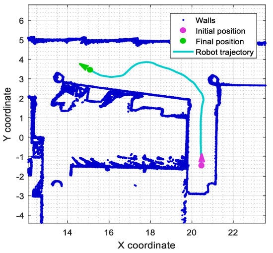
Figure 4.
Reference trajectory of the mobile robot represented on the real 2D map of the experimentation area.
The 2D point cloud map partially depicted in Figure 4 is composed of 10,402 points (blue dots) and was obtained by the mobile robot in a previous exploratory experiment [51]. The starting point (purple dot) defined in the reference trajectory is located near the end of a small, adjacent corridor (Figure 1a). From this position, the robot will perform a short straight displacement until reaching the main corridor. At this point, the robot will proceed to perform a set of soft and hard turns, describing an s-shaped path before reaching the final position (the green point) (see also Figure 1b). The performance of the ICP matching will be evaluated with the APR-02 mobile robot following this challenging reference trajectory in cases with and without stationary obstacles placed along the experimentation area.
2.6. Obstacle Definition
Figure 5 shows the approximate placement of the four stationary obstacles used in this work: A, a rectangular box of 480 × 215 mm; B, a small cylinder with a radius of 42 mm; C, two small cylinders, each with a radius of 50 mm; and D, a medium-sized cylinder with a radius of 135 mm. Each object has been placed in different locations along the corridor and labeled with a number. Each combination of obstacle and position will be used in the validation experiments. The obstacles have been placed in order not to block the reference trajectory of the robot in the different experiments.
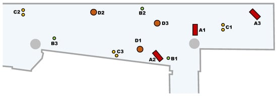
Figure 5.
Depiction of the four different reference stationary obstacles (A, B, C, and D) used in this work. The number in the label identifies each one of the 3 different experiments conducted with an obstacle.
2.7. Performance Metric: Computation Time
The metric used in this work to assess the improvement in execution time is based on monitoring the time taken by the software agent of the mobile robot to complete the following tasks: self-localization in the map (performing ICP matching), path-tracking, obstacle detection, and obstacle evaluation.
The execution time improvement will be computed as:
where is the average computation time required by the software agent implemented in the mobile robot to process 2D LIDAR scans using the original LIBICP [62] library, and is the average computational time required to process the same 2D LIDAR scans using the adapted SLAMICP [61] library developed in this work.
3. ICP Implementation: Returning the Outliers
This section details the new contributions implemented in the SLAMIPC [61] library relative to the reference LIBICP [62] library. The common inputs to both implementations are the 2D point cloud used as a reference or map for the self-localization and the use of the current 2D LIDAR provided by the mobile robot as a partial point cloud . The main differences between these two ICP implementations are the parameters returned. The scope of the new contributions will be highlighted by comparing the MATLAB wrappers provided to call the ICP functions of both libraries.
Figure 6 shows two real scans, M and T, used in this section to illustrate the differences between the LIBICP [62] and SLAMIPC [61] libraries. Figure 6a shows a reference point cloud obtained when the mobile robot is statically located and ready to start an exploration. Figure 6b shows the reference point cloud obtained after the robot has moved. In both cases, these real 2D LIDAR scans are composed of 1081 raw points (blue dots) and represent the contour of the area around the mobile robot in two positions of the application scenario. Note that the scans displayed in Figure 6 are only composed of points, so they may seem noisy in some regions of the contour represented by a few dots. Additionally, the dots representing a plain wall are affected by the measurement error of the real 2D LIDAR, so these dots are not defining perfect flat surfaces.
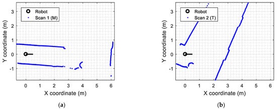
Figure 6.
Real 2D scans gathered from the 2D LIDAR of the mobile robot: (a) the initial scan used as the reference point cloud ; and (b) scan obtained after the mobile robot has moved.
3.1. Reference ICP Matching Library
The MATLAB wrapper that can be used to call the reference LIBICP [62] library is:
where is the transformation matrix () required to match the scan or partial point cloud with the reference point cloud ; is the transformation matrix that describes the last known position of the robot, which is used as an initial guess or approximation, usually this value is the obtained during the previous matching; is a parameter that defines the distance threshold set to determine which points of and will be used as inliers during the matching process, its default value used in this work is 0.3 m; and describes the matching strategy used by the ICP algorithm, which can be either or .
Figure 7 shows the results obtained with the call to this wrapper function implementing ICP matching. Figure 7a shows the representation of the localization of the mobile robot relative to the point cloud , deduced from the values of (see Equation (6)). Additionally, Figure 7b shows the update of the map of the experimentation area obtained by combining all the points of expressed in the coordinates of (adding to with Equation (7)). This updated version of the map describing the experimentation area around the mobile robot used to have thick lines because of the accumulation of successive scans and the inaccuracy of the LIDAR measurements.
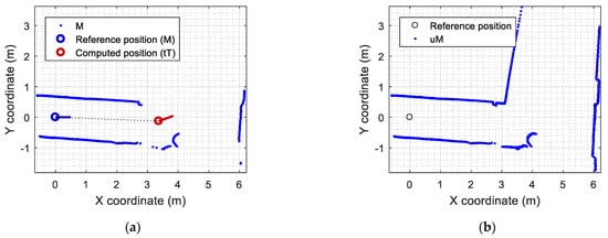
Figure 7.
Results of the ICP matching using the LIBICP library: (a) representation of the self-localization of the mobile robot in the point cloud ; (b) update of the map based on the accumulation of , containing 2162 points.
3.2. ICP Matching Improvement Returning the Outliers
The MATLAB wrapper that can be used to call the ICP matching procedure implemented in the new SLAMICP [61] library is:
This wrapper function has the following new input parameters: is the maximum number of iterations given to the ICP algorithm to find the best solution; is the last known position and orientation of the robot defined as ; and is an optional parameter that enables the definition of a specific distance threshold to detect the outliers after the ICP matching. This parameter is internally initiated to the value specified in the parameter if it is not specified in the call. This parameter provides an additional degree of freedom to differentiate between inliers (points of that have been matched during the ICP procedure) and outliers (points of that have not been matched during the ICP procedure). In this work, the values used for and are 0.3 m.
The new output parameters of the wrapper function are: is the direct estimate of the position and orientation of the robot in the map ; is the number of calls to the iterative fit function performed by the ICP algorithm, is the mean distance of the inlier points after the ICP matching; is a vector containing the indexed position of the points in that have been identified as outliers after the ICP matching, with values in a range from 1 to ; is a 2D matrix containing the coordinates of the outliers detected in already transformed according to so they can be plotted directly over the map and/or added to without requiring additional transformations; is the matrix transformed according the matrix so they can be plotted directly over the map in order to highlight the location of the points of the current scan matched; and is an optional output value that, when requested, contains the concatenation of and in order to automatically generate an updated version of the map . The output parameters are optional and only computed if requested.
The new SLAMICP [61] library also includes MATLAB wrappers with precompiled MEX files and application examples to use this wrapper in the Windows® operating system. The development of the SLAMICP [61] has required the development of specific computer science work with the optimized C++ libraries used, as they were originally designed to return only one parameter as a result of the ICP matching.
Figure 8 shows the application results that can be obtained with the SLAMICP [61] library. Figure 8a shows the representation of the self-localization of the mobile robot relative to the point cloud which is provided directly in as by the library, and the projection of the scan in the map . Figure 8a details the points of the transformed scan that have been identified as shared points or inliers (green points) and the points of the transformed scan that have been identified as outliers (red points), describing new scenario information.
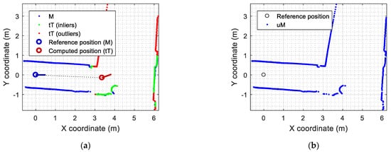
Figure 8.
Results of the ICP matching using the SLAMICP library: (a) representation of the self-localization of the mobile robot in the point cloud detailing the outliers (red points) and inliers (green points) of ; (b) update of the map based on the combination of and the outliers of , in this case containing 1617 points.
The detection of outliers after the ICP matching process can be used to optimize the map-building process. The outliers detected after the ICP matching depict new contour information that is not contained in the map. This means that only the outliers (new information) are merged with the current map. As an illustrative example, Figure 8b shows the result of updating the initial map of the experimentation area (Figure 8a, blue points) with the outliers detected in the current 2D LIDAR scan (Figure 8a, red points). This map-updating process rejects the inliers (Figure 8a, green points) in order to prevent the duplication of information in the map. Consequently, the point cloud map updated with only the outliers (Figure 8b) is composed of thin, clear contour lines. This is not the case when using all the points to compose the map, as any small discrepancy between and will generate a cluster of noisy, redundant points in . Since the ICP algorithm is not capable of filtering noise while building the map, it is important that the map be created without dynamic obstacles.
3.3. Software Agent Implemented in the APR-02 Mobile Robot
This section describes the software agent implemented in the APR-02 mobile robot to perform self-localization, path-tracking, obstacle detection, and obstacle evaluation. This software agent is in charge of calling an ICP matching procedure with the current point cloud gathered by its onboard 2D LIDAR and the 2D map of the application scenario. Additionally, the APR-02 can be configured to create or update a 2D map based on the information from the 2D LIDAR scans, although this procedure requires the definition of special exploratory missions focused on floor coverage [72,73].
Figure 9a presents the original flowchart of the software agent implemented in the APR-02 mobile robot to process the point cloud information provided by the 2D LIDAR scanner. The set of instructions and functions included in the original LIBICP [62] library is outlined with a green, rounded frame. The disadvantage of this original implementation is that the localization of the obstacles in the 2D map requires performing a set of non-optimized subtasks, such as the comparison between the transformed scan and the map to locate discrepancies. This subtask was especially inefficient, as the distance between and was calculated by brute force instead of using an optimized k-d tree such as the one used internally in the LIBICP [62] library. However, the problem detected was that the LIBICP [62] library was not designed to return any other parameter than the transformation matrix of the matching.
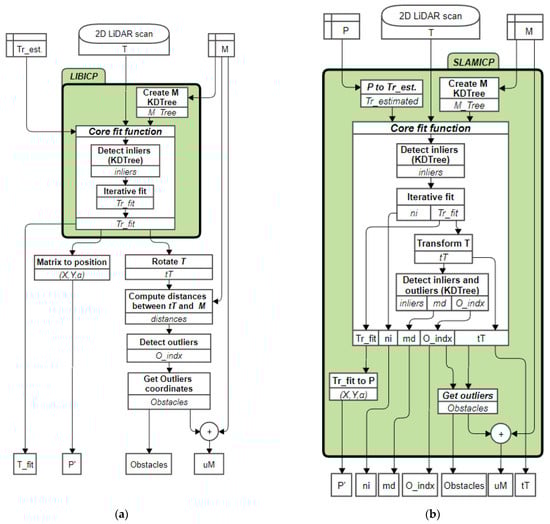
Figure 9.
Flowchart of the software agent processing the 2D LIDAR scans of the APR-02 mobile robot: (a) original implementation based on the LIBICP [62] library; and (b) improved implementation using the adapted SLAMICP [61] library proposed in this work.
A detailed analysis of the software agent presented in Figure 9a suggested the possibility of further improving its efficiency by using the k-d tree classification results. This improvement pointed us in the direction of adapting the LIBICP [62] library to reuse the internal classification of the points of as inliers or outliers. This reuse was identified as an advantage that, for example, will also allow the computation of the distance between and the transformed points of without having to recalculate a new model tree.
Figure 9b shows the flowchart of the software agent based on the use of the new SLAMICP [61] library proposed in this work. The original and improved software agents perform the same subtasks and operations. As stated previously, the main differences are that the SLAMICP [61] library returns the list of outliers provided by the ICP matching algorithm and other matching parameters. This additional information prevents having to repeat time consuming tasks such as computing the distance between and points with the sole purpose of detecting obstacles. Additionally, the SLAMICP [61] library operates in mobile robot coordinates instead of using a transformation matrix and differentiates between outliers and inliers. The performance of the original and adapted software agents will be evaluated in Section 4.
The advantage of the SLAMICP [61] library is that it is fully oriented to mobile robot self-localization and SLAM, allowing the direct estimation of the position and orientation of the robot using the partial point cloud and the map as required inputs. Additionally, the SLAMICP [61] library dynamically determines which output parameters must be generated in order to keep computation time to a minimum. This is achieved by internally defining three different calls to the core ICP matching function.
The first call is designed to implement the basic computations. That is, the calculation of the transformation matrix () that best minimizes the distance between and active points of the template point cloud , from which the new position of the robot can be extracted. This call also retrieves the number of iterations performed by the ICP algorithm before finding the best , a metric that can provide useful information for analyzing the efficiency of the ICP algorithm.
The second call includes the computation of the mean inliers distance (). The inliers are the points of whose distance to the nearest point in is lower than the specified threshold (). This operation requires transforming all the points in according to in order to obtain a transformed point cloud that can be plotted over the map . At this point, the already implemented version of the k-d tree is used to determine the minimum distance between and points. Finally, the mean inlier distance is obtained by dividing the accumulated distance by the number of active points detected in .
The third call is executed in the case of requesting the list detailing the index of the outliers () detected in . In this case, the SLAMICP [61] library allows the definition of a threshold distance for outliers in order to differentiate them from the inliers. Additionally, this call also returns the coordinates of the outliers (). Therefore, there is no need to recalculate the projection of in order to plot and visualize the outliers over the current 2D map .
4. Results
This section presents the results of the different experiments carried out to assess the obstacle detection capabilities and execution time of the new SLAMICP [61] library. During this experimentation phase, the SLAMICP library is used only to identify the position of the robot and does not update or change the map of the area. The obstacles are analyzed based on the outliers (map discrepancies) between the current 2D LIDAR scan and the map retrieved by the SLAMICP library.
4.1. Obstacle Detection Performance at Different Translational Velocities
This section analyzes the number of outliers detected by the ICP matching procedure when the robot moves at a constant translational velocity. This experiment cannot be reproduced with other SLAM implementations, as only the SLAMICP [61] library returns the list of outliers detected. The outliers were detected matching the current 2D LIDAR scan, and a detailed 2D map of the area of experimentation describes the obstacles (or discrepancies) detected. The position of the outliers defines the position of stationary or mobile obstacles around the robot.
As an example, the red dots presented in Figure 10 depict the outliers detected by the mobile robot while following the predefined path defined in Figure 4a. The obstacle used in this experiment is a rectangular box identified with label A2 in Figure 5. Figure 10 shows the evolution of the localization of the outliers detected. In Figure 10a, the mobile robot is about to enter the main corridor, and the obstacle A2 (a rectangular box located near the wall) is barely detected (red points). In Figure 10b, the mobile robot has entered the main corridor, and the outliers detected (red points) fully describe one side of the rectangular box. In Figure 10c, the mobile robot has almost completed the curved trajectory, and the outliers detected (red points) describe the other side of obstacle A2.
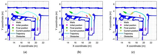
Figure 10.
Representation of the outliers detected (red points) in the corridor (Figure 5, obstacle A2): (a) the robot is about to enter the corridor; (b) the mobile robot has entered in the corridor; (c) the robot has completed most of the planned trajectory.
Figure 11 summarizes the evolution of the number of outliers detected by the ICP algorithm when the mobile robot is configured to repeat the same experiment at different translational velocities. This value is computed from the number of elements provided in , which contains the index of outliers identified by the SLAMIPC [61] library (see Equation (10)). The magenta line in Figure 11 shows the evolution of the outliers when no obstacle is located in the experimentation area. The movement of the robot, along with the inherent measurement errors of the LIDAR sensor, causes the false detection of a reduced number of outliers. The other lines show the evolution of the number of outliers detected when a rectangular box is in the corridor while the robot follows the reference trajectory at different translational velocities, ranging from 0.15 m/s to 0.55 m/s. To simplify the comparison between the different experiments, the y-axis of Figure 11 is set to indicate the distance traveled by the robot, a metric that is independent from the translational velocity of the robot and allows a direct visual comparison of the obtained results. Figure 11 shows that the translational velocity of the mobile robot does not have any remarkable impact on the number of outliers detected during the displacements.
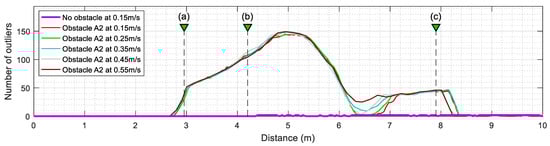
Figure 11.
Evolution of the number of outliers (discrepant points) detected in the LIDAR scans after ICP matching when the mobile robot follows the reference trajectory at different velocities. The labels (a), (b), and (c) identify the positions of the robot depicted in Figure 10. Cases without obstacles (thick magenta line) and with the obstacle A2 (thin lines).
In a complementary way, Figure 12 summarizes the evolution of the mean inlier distance of active points after executing the ICP algorithm. This value is directly the output parameter returned by the SLAMIPC [61] library (see Equation (10)). Figure 12 shows that the evolution of this mean inlier distance is virtually the same regardless of the translational velocity of the robot or the presence of obstacles. This is because the points that could worsen this parameter are classified as outliers and then excluded from the computation of this mean.
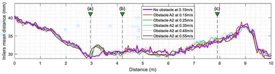
Figure 12.
Evolution of the mean inliers (matched points) distance computed after ICP matching when the mobile robot follows the reference trajectory at different velocities. The labels (a), (b), and (c) identify the position of the robot depicted in Figure 10. Cases without obstacles (thick magenta line) and with the obstacle A2 (thin lines).
Figure 13 shows the evolution of the outliers registered in another example in which the mobile robot follows the reference trajectory (see Figure 4a). In this case, the obstacle used is the small cylinder identified with the label B2 depicted in Figure 5. In Figure 13a, the mobile robot is about to enter the main corridor, and the circular obstacle has already been detected (red points). In Figure 13b, the mobile robot has entered the corridor, and the front side of the circular obstacle is fully detected (red points). In Figure 13c, the mobile robot has completed most of the planned trajectory, and the outliers detected (red points) describe the back-side contour of the obstacle.
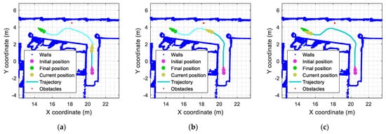
Figure 13.
Detection of a small circular obstacle in the corridor (Figure 5, obstacle B2): (a) the robot is about to enter the corridor; (b) the mobile robot has entered the corridor; (c) the robot has completed most of the planned trajectory.
Similarly, Figure 14 summarizes the evolution of the number of outliers detected by the ICP algorithm, and Figure 15 shows the evolution of the mean inlier distance when the mobile robot is configured to move at different translational velocities. The comparison of the evolution obtained with the obstacles A2 and B2 (Figure 11, Figure 12, Figure 14 and Figure 15) shows that these evolutions do not depend on the translational velocity of the mobile robot.
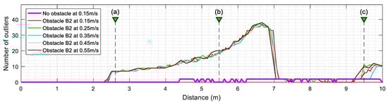
Figure 14.
Evolution of the number of outliers (discrepant points) detected in the LIDAR scans analyzed. Results obtained at different translational velocities of the mobile robot. The labels (a), (b), and (c) identify the positions of the robot depicted in Figure 13. Cases without obstacles (thick magenta line) and with the obstacle B2.

Figure 15.
Evolution of the mean inliers (matched points) distance computed after ICP matching when the mobile robot follows the reference trajectory at different velocities. The labels (a), (b), and (c) identify the positions of the robot is depicted Figure 13. Cases without obstacles (thick magenta line) and with the obstacle B2 (thin lines).
4.2. Obstacle Reconstruction
This section describes the task of reconstructing the obstacles detected around the mobile robot. This reconstruction is based on the accumulation of outliers detected in each scan obtained by the robot during displacements. Figure 16 shows the reconstruction obtained by accumulating the outliers detected in two of the experiments conducted in the previous section. The reconstruction of the obstacles detected can be analyzed offline to determine whether or not the map of the building should be updated. In the case of small obstacles, the list of outliers detected must be filtered in order to provide a sharper reconstruction of the obstacles detected [58,80,81].
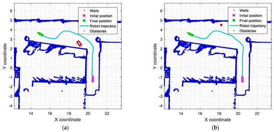
Figure 16a shows the cumulative projection of all the outliers detected during the experiment with the obstacle A2 described in Figure 10, depicting the shape of a rectangular box as an obstacle placed in the corridor. Similarly, Figure 16b shows the cumulative projection of all the outliers detected during the experiment with the obstacle B2 described in Figure 13, depicting the shape of a small circular object placed in the corridor and close to the walls.
At this point, it must be noted that the layout of the floor is prone to change as furniture such as large flowerpots, chair benches, lounge chairs, water fountain machines, advertising stands, and others are often moved around. Then, from time to time, it may be necessary to update the reference map used by the mobile robot in order to accommodate such changes [82].
4.3. Improvement Evaluation
This section assesses the improvement in runtime achieved by the software agent implementing ICP matching in the APR-02 mobile robot. This evaluation compares the computational time taken by the original and proposed software agents to process the same 2D LIDAR scans (see Equation (8)). This evaluation is based on the offline analysis of the scans obtained by the mobile robot following the reference trajectory defined in Figure 4 in the cases including the stationary obstacles defined in Figure 5.
Table 1 shows the obstacles appearing in the trajectory of the mobile robot, the number of experiments performed with each obstacle, the maximum number of outliers detected, and the time taken by the software agent of the mobile robot to complete the following tasks: self-localization in the map (performing ICP matching), path-tracking, obstacle detection, and obstacle evaluation. Two of these experiments have been previously reported in Figure 10, with obstacle A2, and in Figure 13, with obstacle B2. In Table 1, is the average computation time required by the software agent to process one 2D LIDAR scan using the original LIBICP [62] library, and is the average computational time required to process the same 2D LIDAR scans using the adapted SLAMICP [61] library developed in this work. In both cases, the ICP matching strategy is based on a point-to-line metric [21,29].

Table 1.
Mean time spent by the software agent of the APR-02 mobile robot using the LIBICP [62] and the SLAMICP [61] libraries depending on the obstacle appearing in the trajectory of the robot.
The analysis of average values in Table 1 shows that the number of outliers detected in the partial scan does not significantly affect the computational time required by the software agent implemented in the APR-02 mobile robot to process the 2D LIDAR scans. The evaluation of the improvement shows that the use of the adapted SLAMICP [61] library has led to a significant reduction of 36.75% in the average computation time required to process a 2D LIDAR scan by the mobile robot. Basically, this improvement has been achieved by avoiding the need to repeat the calculation of discrepancies between the current scan and the map to detect obstacles around the mobile robot. This procedure is now based on the outliers returned by the SLAMICP [61] library that are processed as discrepancy points defining the localization of obstacles around the mobile robot.
5. Discussion and Conclusions
This work proposes speeding up the detection of obstacles in mobile robot navigation based on monitoring the outliers detected by the ICP matching procedure. The ICP matching algorithm [37] iteratively estimates the transformation matrix that best fits two related point clouds: the 2D LIDAR scan provided by a mobile robot and the 2D map describing the application scenario. The outliers are the points of the 2D LIDAR scan that cannot be matched with any point of the map due to being at a distance greater than a predetermined threshold distance.
In general, obtaining discrepancies between a 2D scan and a 2D map is a time-consuming process that requires the transformation of the 2D scan in order to fit it into the coordinates of the map, the analysis of the matching of the points, and the computation of the distance between points in order to determine which are located at a greater distance than a specified threshold. These time-consuming steps required to compute the variables needed to detect the map discrepancies are the same as the variables already computed during point cloud ICP matching. The SLAMICP [61] library presented in this work has been adapted to return the list of outliers while simultaneously performing localization and mapping. These outliers directly represent map discrepancies and can be monitored to detect obstacles and map changes around the mobile robot. Table 2 provides a comparison between the main features offered by the SLAMICP [61] library and other SLAM library packages such as Hector SLAM [83], Cartographer [84], and the reference LIBICP [62]. The main advantage of the SLAMICP [61] library is its implementation, which is tailored to return the list of outliers detected during ICP matching.
Table 2.
Comparison of the features of the SLAMICP [61] library.
The performance of the software agent using the SLAMICP [61] library for mobile robot self-localization, path tracking, and obstacle detection has been evaluated by defining a reference trajectory composed of a combination of straight and curved displacements and a set of different obstacles.
The results of the experimental evaluation conducted in this work have shown that the number of outliers detected while navigating is not affected by the translational velocity of the mobile robot. Another result obtained is that the mean inlier distance (the distance that defines the overall distance between the matched points) is not affected by the number of outliers because they are discarded and not included in the matching ( discards the point of ). The appreciation of such effects is only possible using an ICP implementation that returns internal information detailing the evolution of the matching procedure. Additionally, the outliers returned after the ICP matching can be cumulated in order to reconstruct the shape of the obstacles detected around the robot, information that can be used to classify the obstacle and decide if the map should be updated.
The final assessment of the APR-02 mobile robot has shown that the computational time required by the software agent processing the 2D LIDAR scans does not change significantly regardless of the number of outliers detected during the ICP matching. This is because the optimized k-d tree search [75] minimizes the computational time required to find the nearest neighbors between two sets of point clouds. Finally, the direct use of the SLAMICP [61] library to detect obstacles has led to a significant reduction of 36.7% in the average computation time required to process the 2D LIDAR scans. This is because monitoring the outliers reported by the ICP algorithm avoids the need to perform redundant analysis in order to detect obstacles (discrepant points between the current scan and the reference map of the application scenario). The implementation of the ICP library developed in this work is freely offered under the GNU General Public License [66] as the SLAMICP [61] library.
Limitations and Future Work
The improvement achieved with the SLAMICP [61] library has been compared with the LIBICP [62] library, which was the ICP matching procedure originally used in the APR-02 mobile robot [85,86]. Future research will address the assessment of the computational performance of the SLAMICP [61] library under other specific layout conditions and hardware usage [87,88,89].
Future developments of the SLAMICP [61] library will address enhancing the performance of the ICP matching in the case of registering a 2D point cloud gathered from a push-broom or articulated 2D LIDAR [38] using a 3D map as a reference and will analyze the correlation between the evolution of the number of outliers detected and the situational awareness achieved in dynamic environments [90]. These developments may allow for improved interpretation of the ICP matching results in crowded and unstructured environments and in multistory navigation.
Author Contributions
Conceptualization, J.P.; formal analysis, E.C.; software, E.C.; supervision, J.P.; writing—original draft, J.P.; writing—review and editing, E.C. All authors have read and agreed to the published version of the manuscript.
Funding
This research received no external funding.
Data Availability Statement
The data used in this work and the SLAMICP library are available at [61]: http://robotica.udl.cat/slamicp/ (accessed on 31 July 2023).
Conflicts of Interest
The authors declare no conflict of interest. The funders had no role in the design of the study; in the collection, analyses, or interpretation of data; in the writing of the manuscript; or in the decision to publish the results.
References
- Borenstein, J.; Everett, H.R.; Feng, L.; Wehe, D. Mobile robot positioning: Sensors and techniques. J. Robot. Syst. 1997, 14, 231–249. [Google Scholar] [CrossRef]
- de Jesús Rubio, J.; Aquino, V.; Figueroa, M. Inverse kinematics of a mobile robot. Neural Comput. Appl. 2013, 23, 187–194. [Google Scholar] [CrossRef]
- Sousa, R.B.; Petry, M.R.; Moreira, A.P. Evolution of Odometry Calibration Methods for Ground Mobile Robots. In Proceedings of the IEEE International Conference on Autonomous Robot Systems and Competitions, Ponta Delgada, Portugal, 15–17 April 2020; pp. 294–299. [Google Scholar] [CrossRef]
- Hijikata, M.; Miyagusuku, R.; Ozaki, K. Wheel Arrangement of Four Omni Wheel Mobile Robot for Compactness. Appl. Sci. 2022, 12, 5798. [Google Scholar] [CrossRef]
- Palacín, J.; Rubies, E.; Clotet, E. Systematic Odometry Error Evaluation and Correction in a Human-Sized Three-Wheeled Omnidirectional Mobile Robot Using Flower-Shaped Calibration Trajectories. Appl. Sci. 2022, 12, 2606. [Google Scholar] [CrossRef]
- Maddahi, Y.; Maddahi, A.; Sepehri, N. Calibration of omnidirectional wheeled mobile robots: Method and experiments. Robotica 2013, 31, 969–980. [Google Scholar] [CrossRef]
- Lin, P.; Liu, D.; Yang, D.; Zou, Q.; Du, Y.; Cong, M. Calibration for Odometry of Omnidirectional Mobile Robots Based on Kinematic Correction. In Proceedings of the 14th International Conference on Computer Science & Education (ICCSE), Toronto, ON, Canada, 19–21 August 2019; pp. 139–144. [Google Scholar] [CrossRef]
- Maulana, E.; Muslim, M.A.; Hendrayawan, V. Inverse kinematic implementation of four-wheels mecanum drive mobile robot using stepper motors. In Proceedings of the 2015 International Seminar on Intelligent Technology and Its Applications, Surabaya, Indonesia, 20–21 May 2015; pp. 51–56. [Google Scholar] [CrossRef]
- Jia, Q.; Wang, M.; Liu, S.; Ge, J.; Gu, C. Research and development of mecanum-wheeled omnidirectional mobile robot implemented by multiple control methods. In Proceedings of the International Conference on Mechatronics and Machine Vision in Practice, Nanjing, China, 28–30 November 2016; pp. 1–4. [Google Scholar] [CrossRef]
- Li, Y.; Ge, S.; Dai, S.; Zhao, L.; Yan, X.; Zheng, Y.; Shi, Y. Kinematic Modeling of a Combined System of Multiple Mecanum-Wheeled Robots with Velocity Compensation. Sensors 2020, 20, 75. [Google Scholar] [CrossRef] [PubMed]
- Savaee, E.; Hanzaki, A.R. A New Algorithm for Calibration of an Omni-Directional Wheeled Mobile Robot Based on Effective Kinematic Parameters Estimation. J. Intell. Robot. Syst. 2021, 101, 28. [Google Scholar] [CrossRef]
- Palacín, J.; Rubies, E.; Bitrià, R.; Clotet, E. Non-Parametric Calibration of the Inverse Kinematic Matrix of a Three-Wheeled Omnidirectional Mobile Robot Based on Genetic Algorithms. Appl. Sci. 2023, 13, 1053. [Google Scholar] [CrossRef]
- Reina, G.; Ojeda, L.; Milella, A.; Borenstein, J. Wheel slippage and sinkage detection for planetary rovers. IEEE/ASME Trans. Mechatron. 2006, 11, 185–195. [Google Scholar] [CrossRef]
- Cho, B.S.; Moon, W.S.; Seo, W.J.; Baek, K.R. A dead reckoning localization system for mobile robots using inertial sensors and wheel revolution encoding. J. Mech. Sci. Technol. 2011, 25, 2907–2917. [Google Scholar] [CrossRef]
- Jin, J.; Chung, W. Obstacle Avoidance of Two-Wheel Differential Robots Considering the Uncertainty of Robot Motion on the Basis of Encoder Odometry Information. Sensors 2019, 19, 289. [Google Scholar] [CrossRef]
- Palacín, J.; Martínez, D. Improving the Angular Velocity Measured with a Low-Cost Magnetic Rotary Encoder Attached to a Brushed DC Motor by Compensating Magnet and Hall-Effect Sensor Misalignments. Sensors 2021, 21, 4763. [Google Scholar] [CrossRef]
- Aqel, M.O.A.; Marhaban, M.H.; Saripan, M.I.; Ismail, N.B. Review of visual odometry: Types, approaches, challenges, and applications. SpringerPlus 2016, 5, 1897. [Google Scholar] [CrossRef]
- Bârsan, I.A.; Liu, P.; Pollefeys, M.; Geiger, A. Robust dense mapping for large-scale dynamic environments. In Proceedings of the IEEE International Conference on Robotics and Automation, Brisbane, QLD, Australia, 21–25 May 2018; pp. 7510–7517. [Google Scholar] [CrossRef]
- Ji, K.; Chen, H.; Di, H.; Gong, J.; Xiong, G.; Qi, J.; Yi, T. CPFG-SLAM: A robust simultaneous localization and mapping based on LIDAR in off-road environment. In Proceedings of the IEEE Intelligent Vehicles Symposium, Changshu, China, 26–30 June 2018; pp. 650–655. [Google Scholar] [CrossRef]
- Du, S.; Li, Y.; Li, X.; Wu, M. LiDAR Odometry and Mapping Based on Semantic Information for Outdoor Environment. Remote Sens. 2021, 13, 2864. [Google Scholar] [CrossRef]
- Chen, Y.; Medioni, G. Object modeling by registration of multiple range images. IEEE Int. Conf. Robot. Autom. 1991, 3, 2724–2729. [Google Scholar] [CrossRef]
- Yokozuka, M.; Koide, K.; Oishi, S.; Banno, A. LiTAMIN: LiDAR-Based Tracking and Mapping by Stabilized ICP for Geometry Approximation with Normal Distributions. In Proceedings of the IEEE/RSJ International Conference on Intelligent Robots and Systems (IROS), Las Vegas, NV, USA, 25–29 October 2020; pp. 5143–5150. [Google Scholar] [CrossRef]
- Koide, K.; Miura, J.; Menegatti, E. A portable three-dimensional LIDAR-based system for long-term and wide-area people behavior measurement. Int. J. Adv. Robot. Syst. 2019, 1–16. [Google Scholar] [CrossRef]
- Behley, J.; Stachniss, C. Efficient Surfel-Based SLAM using 3D Laser Range Data in Urban Environments. In Proceedings of the International Conference on Robotics: Science and Systems (RSS), Pittsburgh, Pennsylvania, USA, 26–30 June 2018. [Google Scholar] [CrossRef]
- Park, C.; Moghadam, P.; Kim, S.; Elfes, A.; Fookes, C.; Sridharan, S. Elastic LiDAR Fusion: Dense Map-Centric Continuous-Time SLAM. In Proceedings of the International Conference on Robotics and Automation (ICRA), Brisbane, Australia, 21–25 May 2017. [Google Scholar] [CrossRef]
- Whelan, T.; Leutenegger, S.; Moreno, R.; Glocker, B.; Davison, A. ElasticFusion: Dense SLAM Without A Pose Graph. In Proceedings of the International Conference of Robotics: Science and Systems (RSS), Rome, Italy, 13–17 July 2015. [Google Scholar] [CrossRef]
- Moosmann, F.; Stiller, C. Velodyne SLAM. In Proceedings of the IEEE Intelligent Vehicles Symposium (IV), Baden-Baden, Germany, 5–9 June 2011. [Google Scholar] [CrossRef]
- Droeschel, D.; Behnke, S. Efficient Continuous-time SLAM for 3D Lidar-based Online Mapping. In Proceedings of the International Conference on Robotics and Automation (ICRA), Brisbane, Australia, 21–25 May 2018. [Google Scholar] [CrossRef]
- Besl, P.J.; McKay, N.D. A Method for Registration of 3-D Shapes. IEEE Trans. Pattern Anal. Mach. Intell. 1992, 14, 239–256. [Google Scholar] [CrossRef]
- Zhang, J.; Singh, S. LOAM: Lidar Odometry and Mapping in Real-time. In Proceedings of the International Conference of Robotics: Science and Systems (RSS), Berkeley, CA, USA, 12–16 July 2014. [Google Scholar] [CrossRef]
- Zhang, J.; Singh, S. Low-drift and Real-time Lidar Odometry and Mapping. Auton. Robot. 2017, 41, 401–416. [Google Scholar] [CrossRef]
- Shan, T.; Englot, B. LeGO-LOAM: Lightweight and Ground-Optimized Lidar Odometry and Mapping on Variable Terrain. In Proceedings of the International Conference on Intelligent Robots and Systems (IROS), Madrid, Spain, 1–5 October 2018. [Google Scholar] [CrossRef]
- Ye, H.; Chen, Y.; Liu, M. Tightly Coupled 3D Lidar Inertial Odometry and Mapping. In Proceedings of the International Conference on Robotics and Automation, Montreal, QC, Canada, 20–24 May 2019; pp. 3144–3150. [Google Scholar] [CrossRef]
- Shan, T.; Englot, B.; Meyers, D.; Wang, W.; Ratti, C.; Rus, D. LIO-SAM: Tightly-coupled Lidar Inertial Odometry via Smoothing and Mapping. In Proceedings of the International Conference on Intelligent Robots and Systems (IROS), Las Vegas, NV, USA, 25–29 October 2020. [Google Scholar] [CrossRef]
- Qin, C.; Ye, H.; Pranata, C.E.; Han, J.; Zhang, S.; Liu, M. LINS: A Lidar-Inertial State Estimator for Robust and Efficient Navigation. In Proceedings of the IEEE International Conference on Robotics and Automation (ICRA), Virtual (Online), 31 May–31 August 2020. [Google Scholar] [CrossRef]
- LeCun, Y.; Bengio, Y.; Hinton, G. Deep Learning. Nature 2015, 521, 436–444. [Google Scholar] [CrossRef] [PubMed]
- Pomerleau, F.; Colas, F.; Siegwart, R. A Review of Point Cloud Registration Algorithms for Mobile Robotics. Found. Trends Robot. 2015, 4, 1–104. [Google Scholar] [CrossRef]
- Palacín, J.; Martínez, D.; Rubies, E.; Clotet, E. Mobile Robot Self-Localization with 2D Push-Broom LIDAR in a 2D Map. Sensors 2020, 20, 2500. [Google Scholar] [CrossRef]
- Bhandari, V.; Phillips, T.G.; McAree, P.R. Real-Time 6-DOF Pose Estimation of Known Geometries in Point Cloud Data. Sensors 2023, 23, 3085. [Google Scholar] [CrossRef]
- He, Y.; Liang, B.; Yang, J.; Li, S.; He, J. An Iterative Closest Points Algorithm for Registration of 3D Laser Scanner Point Clouds with Geometric Features. Sensors 2017, 17, 1862. [Google Scholar] [CrossRef] [PubMed]
- Jung, Y.; Jeon, M.; Kim, C.; Seo, S.-W.; Kim, S.-W. Uncertaintyaware fast curb detection using convolutional networks in point clouds. In Proceedings of the IEEE International Conference on Robotics and Automation (ICRA), Xi’an, China, 30 May–5 June 2021; pp. 12882–12888. [Google Scholar] [CrossRef]
- Zheng, C.; Lyu, Y.; Li, M.; Zhang, Z. Lodonet: A deep neural network with 2d keypoint matching for 3d lidar odometry estimation. In Proceedings of the ACM International Conference on Multimedia, Virtual Conference, 12–16 October 2020; pp. 2391–2399. [Google Scholar] [CrossRef]
- Li, Z.; Wang, N. Dmlo: Deep matching lidar odometry. In Proceedings of the IEEE/RSJ International Conference on Intelligent Robots and Systems, Virtual Conference, 25–29 October 2020; pp. 6010–6017. [Google Scholar] [CrossRef]
- Li, Q.; Chen, S.; Wang, C.; Li, X.; Wen, C.; Cheng, M.; Li, J. Lonet: Deep real-time lidar odometry. In Proceedings of the IEEE/CVF Conference on Computer Vision and Pattern Recognition, Long Beach, CA, USA, 15–20 June 2019; pp. 8473–8482. [Google Scholar] [CrossRef]
- Nubert, J.; Khattak, S.; Hutter, M. Self-supervised learning of lidar odometry for robotic applications. In Proceedings of the IEEE International Conference on Robotics and Automation 2021, Motreal, QC, Canada, 20–24 May 2019; pp. 9601–9607. [Google Scholar] [CrossRef]
- Wang, M.; Saputra, R.U.; Zhao, P.; Gusmao, P.; Yang, B.; Chen, C.; Markham, A.; Trigoni, N. Deeppco: End-to-end point cloud odometry through deep parallel neural network. In Proceedings of the IEEE/RSJ International Conference on Intelligent Robots and Systems 2019, Macau, China, 4–8 November 2019; pp. 3248–3254. [Google Scholar] [CrossRef]
- Cho, Y.; Kim, G.; Kim, A. Unsupervised geometry-aware deep lidar odometry. In Proceedings of the IEEE International Conference on Robotics and Automation 2020, Paris, France, 31 May–31 August 2020; pp. 2145–2152. [Google Scholar] [CrossRef]
- Wang, G.; Wu, X.; Liu, Z.; Wang, H. Pwclo-net: Deep lidar odometry in 3d point clouds using hierarchical embedding mask optimization. In Proceedings of the IEEE/CVF Conference on Computer Vision and Pattern Recognition, Virtual Conference, 19–25 June 2021; pp. 15910–15919. [Google Scholar] [CrossRef]
- Jung, D.; Cho, J.-K.; Jung, Y.; Shin, S.; Kim, S.-W. LoRCoN-LO: Long-term Recurrent Convolutional Network-based LiDAR Odometry. In Proceedings of the International Conference on Electronics, Information, and Communication, Singapore, 5–8 February 2023; pp. 1–4. [Google Scholar] [CrossRef]
- Hess, W.; Kohler, D.; Rapp, H.; Andor, D. Real-time loop closure in 2D LIDAR SLAM. In Proceedings of the IEEE International Conference on Robotics and Automation (ICRA), Stockholm, Sweden, 16–20 May 2016; pp. 1271–1278. [Google Scholar] [CrossRef]
- Lluvia, I.; Lazkano, E.; Ansuategi, A. Active Mapping and Robot Exploration: A Survey. Sensors 2021, 21, 2445. [Google Scholar] [CrossRef] [PubMed]
- Nagla, S. 2D Hector SLAM of Indoor Mobile Robot using 2D LIDAR. In Proceedings of the International Conference on Power, Energy, Control 472 and Transmission Systems (ICPECTS), Chennai, India, 10–11 December 2020. [Google Scholar] [CrossRef]
- Tee, Y.K.; Han, Y.C. Lidar-Based 2D SLAM for Mobile Robot in an Indoor Environment: A Review. In Proceedings of the International Conference on Green Energy, Computing and Sustainable Technology (GECOST), Miri, Malaysia, 7–9 July 2021; p. 475. [Google Scholar] [CrossRef]
- Mendes, E.; Koch, P.; Lacroix, S. ICP-based pose-graph SLAM. In Proceedings of the IEEE International Symposium on Safety, Security, and Rescue Robotics (SSRR), Lausanne, Switzerland, 23–27 October 2016; pp. 195–200. [Google Scholar] [CrossRef]
- Guiotte, F.; Lefèvre, S.; Corpetti, T. Attribute Filtering of Urban Point Clouds Using Max-Tree on Voxel Data. In Mathematical Morphology and Its Applications to Signal and Image Processing; Lecture Notes in Computer Science; Burgeth, B., Kleefeld, A., Naegel, B., Passat, N., Perret, B., Eds.; Springer: Cham, Switzerland, 2019; Volume 11564. [Google Scholar] [CrossRef]
- Yuan, C.; Xu, W.; Liu, X.; Hong, X.; Zhang, F. Efficient and Probabilistic Adaptive Voxel Mapping for Accurate Online LiDAR Odometry. IEEE Robot. Autom. Lett. 2022, 7, 8518–8525. [Google Scholar] [CrossRef]
- Rusinkiewicz, S.; Levoy, M. Efficient variants of the ICP algorithm. In Proceedings of the International Conference on 3D Digital Imaging and Modeling (3DIM), Quebec City, QC, Canada, 28 May–1 June 2001. [Google Scholar] [CrossRef]
- Borenstein, J.; Koren, Y. The vector field histogram-fast obstacle avoidance for mobile robots. IEEE Trans. Robot. Autom. 1991, 7, 278–288. [Google Scholar] [CrossRef]
- Sezer, V.; Gokasan, M. A novel obstacle avoidance algorithm: “Follow the Gap Method”. Robot. Auton. Syst. 2012, 60, 1123–1134. [Google Scholar] [CrossRef]
- Rostami, S.M.H.; Sangaiah, A.K.; Wang, J.; Liu, X. Obstacle avoidance of mobile robots using modified artificial potential field algorithm. J. Wirel. Com. Netw. 2019, 2019, 70. [Google Scholar] [CrossRef]
- SLAMICP: C++ Library for Iterative Closest Point Matching. Available online: http://robotica.udl.cat/slamicp/ (accessed on 30 June 2023).
- LIBICP: C++ Library for Iterative Closest Point Matching. Available online: https://www.cvlibs.net/software/libicp/ (accessed on 17 March 2023).
- Geiger, A.; Lenz, P.; Urtasun, R. Are we ready for Autonomous Driving? In Proceedings of the KITTI Vision Benchmark Suite, Conference on Computer Vision and Pattern Recognition, Providence, RI, USA, 26 July 2012. [Google Scholar] [CrossRef]
- Geiger, A.; Lenz, P.; Stiller, C.; Urtasun, R. Vision meets robotics: The KITTI dataset. Int. J. Robot. Res. 2013, 32, 1231–1237. [Google Scholar] [CrossRef]
- KITTI Vision Benchmark Suite. Available online: https://www.cvlibs.net/datasets/kitti/ (accessed on 17 March 2023).
- GNU General Public License. Available online: https://www.gnu.org/licenses/gpl-3.0.html (accessed on 17 April 2023).
- Palacín, J.; Rubies, E.; Clotet, E. The Assistant Personal Robot Project: From the APR-01 to the APR-02 Mobile Robot Prototypes. Designs 2022, 6, 66. [Google Scholar] [CrossRef]
- Palacín, J.; Martínez, D.; Clotet, E.; Pallejà, T.; Burgués, J.; Fonollosa, J.; Pardo, A.; Marco, S. Application of an Array of Metal-Oxide Semiconductor Gas Sensors in an Assistant Personal Robot for Early Gas Leak Detection. Sensors 2019, 19, 1957. [Google Scholar] [CrossRef] [PubMed]
- Rubies, E.; Palacín, J.; Clotet, E. Enhancing the Sense of Attention from an Assistance Mobile Robot by Improving Eye-Gaze Contact from Its Iconic Face Displayed on a Flat Screen. Sensors 2022, 22, 4282. [Google Scholar] [CrossRef] [PubMed]
- Rubies, E.; Palacín, J. Design and FDM/FFF Implementation of a Compact Omnidirectional Wheel for a Mobile Robot and Assessment of ABS and PLA Printing Materials. Robotics 2020, 9, 43. [Google Scholar] [CrossRef]
- Bitriá, R.; Palacín, J. Optimal PID Control of a Brushed DC Motor with an Embedded Low-Cost Magnetic Quadrature Encoder for Improved Step Overshoot and Undershoot Responses in a Mobile Robot Application. Sensors 2022, 22, 7817. [Google Scholar] [CrossRef]
- Durrant-Whyte, H.; Bailey, T. Simultaneous localization and mapping: Part I. IEEE Robot. Autom. Mag. 2006, 13, 99–110. [Google Scholar] [CrossRef]
- Bailey, T.; Durrant-Whyte, H. Simultaneous localization and mapping: Part II. IEEE Robot. Autom. Mag. 2006, 13, 108–117. [Google Scholar] [CrossRef]
- Eade, E.; Fong, P.; Munich, M.E. Monocular graph SLAM with complexity reduction. In Proceedings of the IEEE/RSJ International Conference on Intelligent Robots and Systems, Taipei, Taiwan, 18–22 October 2010; pp. 3017–3024. [Google Scholar] [CrossRef]
- Louis, J. Multidimensional binary search trees used for associative searching. Commun. ACM 1975, 18, 509–517. [Google Scholar] [CrossRef]
- Boost C++ Libraries. Available online: Boost.org (accessed on 26 January 2023).
- Chetverikov, D.; Svirko, D.; Stepanov, D.; Krsek, P. The Trimmed Iterative Closest Point algorithm. In Proceedings of the International Conference on Pattern Recognition, Quebec City, QC, Canada, 11–15 August 2002; Volume 3, pp. 545–548. [Google Scholar] [CrossRef]
- Sánchez-Ibáñez, J.R.; Pérez-del-Pulgar, C.J.; García-Cerezo, A. Path Planning for Autonomous Mobile Robots: A Review. Sensors 2021, 21, 7898. [Google Scholar] [CrossRef] [PubMed]
- Palacín, J.; Rubies, E.; Clotet, E.; Martínez, D. Evaluation of the Path-Tracking Accuracy of a Three-Wheeled Omnidirectional Mobile Robot Designed as a Personal Assistant. Sensors 2021, 21, 7216. [Google Scholar] [CrossRef]
- Hu, W.; Zhang, K.; Shao, L.; Lin, Q.; Hua, Y.; Qin, J. Clustering Denoising of 2D LiDAR Scanning in Indoor Environment Based on Keyframe Extraction. Sensors 2023, 23, 18. [Google Scholar] [CrossRef]
- Charron, N.; Phillips, S.; Waslander, S.L. De-noising of Lidar Point Clouds Corrupted by Snowfall. In Proceedings of the Conference on Computer and Robot Vision (CRV), Toronto, ON, Canada, 8–10 May 2018; pp. 254–261. [Google Scholar] [CrossRef]
- Banerjee, N.; Lisin, D.; Lenser, S.R.; Briggs, J.; Baravalle, R.; Albanese, V.; Chen, Y.; Karimian, A.; Ramaswamy, T.; Pilotti, P.; et al. Lifelong mapping in the wild: Novel strategies for ensuring map stability and accuracy over time evaluated on thousands of robots. Robot. Auton. Syst. 2023, 164, 104403. [Google Scholar] [CrossRef]
- Hector SLAM. Available online: http://wiki.ros.org/hector_slam (accessed on 30 June 2023).
- Cartographer. Available online: https://github.com/cartographer-project/cartographer (accessed on 30 June 2023).
- Minguez, J.; Lamiraux, F.; Montesano, L. Metric-Based Scan Matching Algorithms for Mobile Robot Displacement Estimation. In Proceedings of the 2005 IEEE International Conference on Robotics and Automation, Barcelona, Spain, 18–22 April 2005; pp. 3557–3563. [Google Scholar] [CrossRef]
- Montesano, L.; Minguez, J.; Montano, L.A. Lessons Learned in Integration for Sensor-Based Robot Navigation Systems. Int. J. Adv. Robot. Syst. 2006, 3, 15. [Google Scholar] [CrossRef]
- Lee, D.; Kim, H.; Myung, H. GPU-based real-time RGB-D 3D SLAM. In Proceedings of the International Conference on Ubiquitous Robots and Ambient Intelligence, Daejeon, Republic of Korea, 26–28 November 2012; pp. 46–48. [Google Scholar] [CrossRef]
- Ratter, A.; Sammut, C.; McGill, M. GPU accelerated graph SLAM and occupancy voxel based ICP for encoder-free mobile robots. In Proceedings of the IEEE/RSJ International Conference on Intelligent Robots and Systems, Tokyo, Japan, 3–7 November 2013; pp. 540–547. [Google Scholar] [CrossRef]
- Aldegheri, S.; Bombieri, N.; Bloisi, D.D.; Farinelli, A. Data Flow ORB-SLAM for Real-time Performance on Embedded GPU Boards. In Proceedings of the IEEE/RSJ International Conference on Intelligent Robots and Systems, Macau, China, 3–8 November 2019; pp. 5370–5375. [Google Scholar] [CrossRef]
- Bavle, H.; Sanchez-Lopez, J.L.; Cimarelli, C.; Tourani, A.; Voos, H. From SLAM to Situational Awareness: Challenges and Survey. Sensors 2023, 23, 4849. [Google Scholar] [CrossRef] [PubMed]
Disclaimer/Publisher’s Note: The statements, opinions and data contained in all publications are solely those of the individual author(s) and contributor(s) and not of MDPI and/or the editor(s). MDPI and/or the editor(s) disclaim responsibility for any injury to people or property resulting from any ideas, methods, instructions or products referred to in the content. |
© 2023 by the authors. Licensee MDPI, Basel, Switzerland. This article is an open access article distributed under the terms and conditions of the Creative Commons Attribution (CC BY) license (https://creativecommons.org/licenses/by/4.0/).