Predicting the Early-Age Time-Dependent Behaviors of a Prestressed Concrete Beam by Using Physics-Informed Neural Network

Abstract

This paper proposes a physics-informed neural network (PINN) for predicting the early-age time-dependent behaviors of prestressed concrete beams. The PINN utilizes deep neural networks to learn the time-dependent coupling among the effective prestress force and the several factors that affect the time-dependent behavior of the beam, such as concrete creep and shrinkage, tendon relaxation, and changes in concrete elastic modulus. Unlike traditional numerical algorithms such as the finite difference method, the PINN directly solves the integro-differential equation without the need for discretization, offering an efficient and accurate solution. Considering the trade-off between solution accuracy and the computing cost, optimal hyperparameter combinations are determined for the PINN. The proposed PINN is verified through the comparison to the numerical results from the finite difference method for two representative cross sections of PSC beams.

1. Introduction

Most machine learning-based approaches for predicting the mechanical behaviors of structural systems require a huge amount of high-quality data for supervised learning. In many real-world engineering problems, such vast amounts of data are often unattainable on site, and limitations in data accessibility pose challenges for machine learning based on field data. To overcome these limitations, the physics-informed neural network (PINN) has gained attention for its capability of incorporating fundamental physical (or mechanical) knowledge, presented in the form of differential or integral equations, into machine learning [1,2,3,4,5,6,7,8].

The PINN addresses data limitation challenges by excelling in solving problems with uncertain or missing information [9] and holds the potential to significantly reduce computational costs [10]. Additionally, the PINN can be applied to problems in arbitrary domains and can scale to high-dimensional systems. In numerous scientific and engineering fields, the PINN is gaining increasing popularity today including material [11,12,13], nonlinear diffusivity [14], fluid mechanics [15,16,17,18], bioengineering [19], solid mechanics [20,21], geophysics [22], thermophysics [23], machine fault diagnosis [24], and scientific computations [25,26]. Furthermore, the PINN has been expanded to tackle integro-differential equations (IDEs) [27], fractional differential equations (FDEs) [28], stochastic differential equations (SDEs) [29,30,31,32], and shown to estimate the generalization error [33,34,35].

The PINN utilizes a feed-forward architecture combined with automated differentiation in artificial neural networks to train models that satisfy the governing equations, enabling the construction of physical prediction models with far fewer field data than traditional data-driven neural network techniques [36]. The PINN estimates the parameters that make up the neural network by optimizing an objective function composed of errors related to the governing equations and boundary (or initial) conditions. In this process, it is necessary to calculate the derivative values for the unknowns included in the governing equations or boundary conditions, and the PINN adopts automatic differentiation techniques instead of numerical differentiation [37]. This advantage allows for the direct handling of any form of differential operators for unknowns included in the governing equations. By using PINNs, it is possible to address the missing data and measurement errors in actual physics that could not be resolved with conventional approaches.

PINNs demonstrate constraints when handling issues that evolve sharp gradients or involve interconnected PDEs [38]. As a consequence, traditional PINNs have been improved by employing domain decomposition methods [39,40,41,42]. A generalized space-time domain decomposition framework for PINNs (XPINN) was proposed to solve any differential equations on arbitrary complex geometry domains [39,40]. The XPINN easily lends itself to space-time parallelization, thereby reducing training costs more effectively. Augmented PINN (APINN) was proposed to further improve the XPINN as well as vanilla PINNs by adopting soft and trainable domain decomposition and flexible parameter sharing [41]. The domain decomposition methods can reduce the complexity of PINNs by dividing the problem into smaller, more manageable subproblems. They also can improve the stability of PINNs by reducing the risk of overfitting since the subproblems are more independent, which can help to prevent the model from learning spurious correlations.

The incorporation of adaptive activation functions into traditional PINNs has emerged as a compelling alternative [43,44,45,46]. Adaptive activation functions can help PINNs to converge more quickly and reliably because they can adapt to the specific problem at hand, which can help to avoid getting stuck in local minima. They also can help PINNs to generalize better to unseen data since they can learn to represent the underlying physical laws more accurately improving the robustness of the model. Lastly, they can be less sensitive to hyperparameters than conventional activation functions. This is because they can adapt to the specific problem at hand, which can help to improve the stability of the training process.

In the civil engineering industry, prestressed concrete (PSC) beams are increasingly used in construction due to their advantages over reinforced concrete (RC) beams in controlling cracking and minimizing long-term deflections [47]. To design safe and reliable PSC beams, however, it is crucial to properly predict prestress losses, particularly in high-strength concrete, at an early age [48,49,50]. There have been numerous attempts to investigate the time-dependent behavior of PSC structures, including the effects of concrete creep and shrinkage, tendon relaxation, and changes in the concrete elastic modulus [51,52,53,54,55,56]. Most of these studies employ numerical models such as finite element and finite difference methods to predict the long-term behavior of prestressed concrete structures [57,58,59,60]. They are computationally intensive and require significant computational resources.

This paper presents a PINN-based approach for predicting the early-age time-dependent behaviors of a PSC beam considering interaction among concrete creep and shrinkage, tendon relaxation, and the changes of concrete elastic modulus. We introduce a novel closed-form integro-differential governing equation, formulated in terms of effective prestress force, to predict the early-age time-dependent behaviors of PSC beams. Contrary to the traditional finite element method, the PINN directly solves the integro-differential equation without requiring discretization. There exists a trade-off between solution accuracy and the computing time when solving the integro-differential governing equation through PINN. Balancing the importance of the solution accuracy and the computing cost, optimal hyperparameter combinations are determined for the PINN.

The paper is organized as follows. Section 2.1 presents eight dimensionless governing equations for the time-dependent behaviors of a PSC beam. Section 2.2 describes the derivation of the closed-form integro-differential equation in terms of dimensionless effective prestress force. Section 2.3 presents determining optimal hyperparameter combinations for the PINN to solve the integro-differential equation. Section 3.1 presents the results of optimal hyperparameter combinations for the PINN and a comparison with the finite difference method for PSC beams with rectangular and I-shaped cross sections. Finally, Section 4 summarizes the findings and their implications for the proposed PINN approach.

2. Materials and Methods

2.1. Governing Equations

2.1.1. Problem Definition and Assumptions

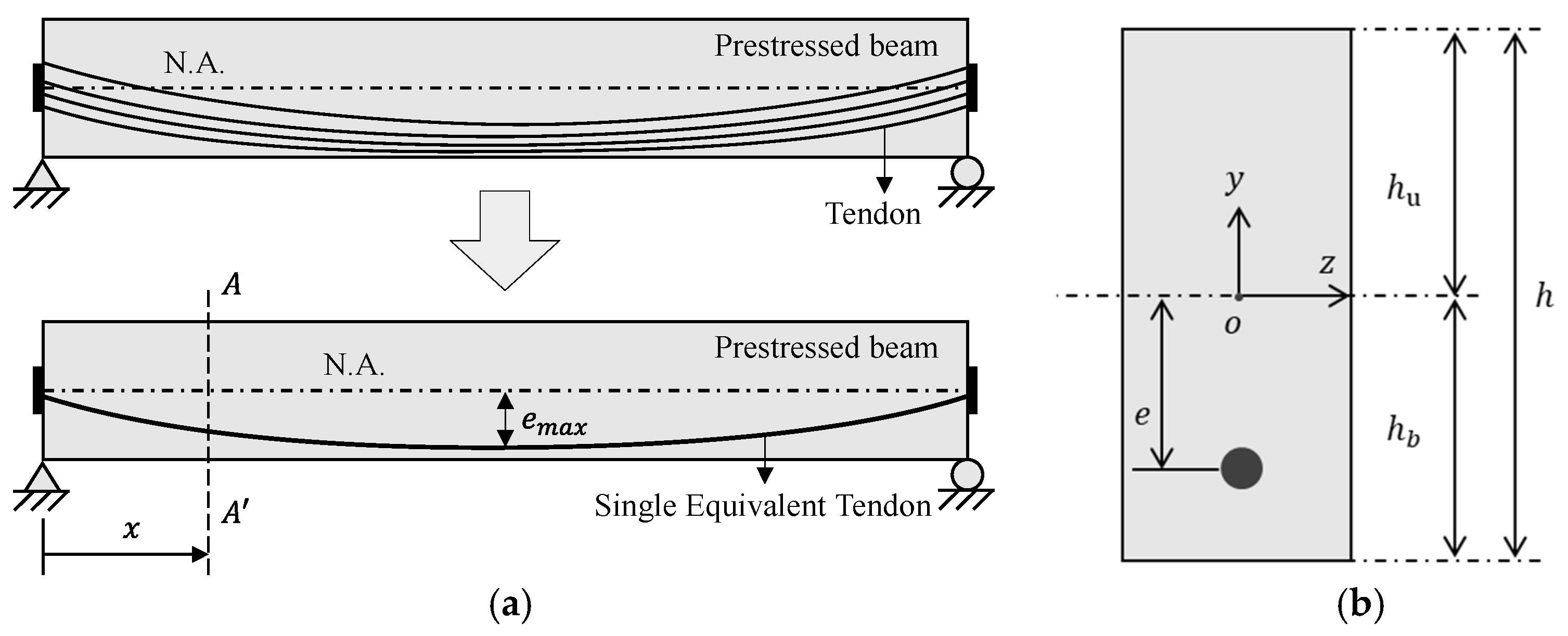
Figure 1 presents a simplified PSC beam model to analyze the early-age time-dependent behaviors of a precast prestressed concrete beam. The period of interest for the analysis spans approximately one year beginning from the initial prestress transfer to the installation of the beam at the intended target construction site. The assumptions for the time-dependent analysis of this study can be described as follows:

(i) Multiple tendons of the PSC beam can be substituted with a single equivalent tendon as shown in Figure 1a;

(ii) The tendon is perfectly bonded with concrete; thus, section analysis for equilibrium between the tendon and the concrete is possible;

(iii) The beam model follows the Euler–Bernoulli beam theory;

(vi) The time-dependent behaviors of concrete include the change of elastic modulus, creep, and shrinkage;

(v) The creep of concrete follows the standard linear model of viscoelasticity;

(vi) The relaxation of the tendon is assumed to be intrinsic;

(vii) The shrinkage of concrete occurs uniformly throughout the gross section of concrete;

(viii) The net strain of concrete consists of elastic strain, creep strain, and shrinkage strain;

(ix) The self-weight of the PSC beam is introduced at the moment of initial prestress transfer.

Figure 1. Simplified beam model for a PSC beam: (a) PSC beam model with a single equivalent tendon; (b) cross section at $A{A}^{\prime }$.

Figure 1. Simplified beam model for a PSC beam: (a) PSC beam model with a single equivalent tendon; (b) cross section at $A{A}^{\prime }$.

2.1.2. Governing Equations for Time-Dependent Behaviors of a PSC Beam

In the simplified model for a PSC beam in Figure 1, a time-dependent analysis should be conducted at each section of interest to satisfy the equilibrium between the concrete and the tendon. For the simplicity of description, the spatial variable $x$ corresponding to section $A{A}^{\prime }$ in Figure 1 is omitted in all field variables hereafter.

The governing equations for time-dependent behaviors can be expressed as follows:

(i) Axial-bending stress equation of concrete

$$\sigma \left(y,t\right)=-P\left(t\right)\left(\frac{1}{A_{\mathrm{c}}}-\frac{e}{I_{\mathrm{c}}}y\right)-\frac{M_{\mathrm{d}}}{I_{\mathrm{c}}}y$$

(1)

where $t$ and $M_{\mathrm{d}}$ denote the time beginning from the initial prestress transfer and the bending moment induced by the self-weight of the beam, respectively.

(ii) Constitutive equation of elastic strain of concrete [61]

$$\begin{array}{cc}\hfill {\epsilon }_{\mathrm{el}}\left(y,t\right)=\frac{\sigma \left(y,t\right)}{E_{\mathrm{c}}\left(t\right)}& ={\mathsf{\Phi }}_{\mathrm{el}}\left(t\right)\frac{\sigma \left(y,t\right)}{E_{\mathrm{c}0}}\hfill \\ \hfill & =-{\mathsf{\Phi }}_{\mathrm{el}}\left(t\right)P\left(t\right)\left(\frac{1}{E_{\mathrm{c}0}{A}_{\mathrm{c}}}-\frac{e}{E_{\mathrm{c}0}{I}_{\mathrm{c}}}y\right)-{\mathsf{\Phi }}_{\mathrm{el}}\left(t\right)\frac{M_{\mathrm{d}}}{E_{\mathrm{c}0}{I}_{\mathrm{c}}}y\hfill \end{array}$$

(2)

where $E_{\mathrm{c}0}$ is the elastic modulus of concrete at $t=0$ and ${\mathsf{\Phi }}_{\mathrm{el}}\left(t\right)=\frac{E_{\mathrm{c}0}}{E_{\mathrm{c}}\left(t\right)}$.

(iii) Constitutive equation of creep strain of concrete [62]

$${\epsilon }_{\mathrm{cr}}\left(y,t\right)={{\displaystyle \int }}_0^t\frac{{\tilde{\mathsf{\Phi }}}_{\mathrm{cr}}\left(t,\tau \right)}{E_{\mathrm{ci}}}\frac{\partial \sigma \left(y,\tau \right)}{\partial \tau }d\tau +\frac{{\tilde{\mathsf{\Phi }}}_{\mathrm{cr}}\left(t,0\right)}{E_{\mathrm{ci}}}\sigma \left(y,0\right)$$

(3)

where $E_{\mathrm{ci}}$ is the elastic modulus of concrete at the age of 28 days while ${\tilde{\mathsf{\Phi }}}_{\mathrm{cr}}\left(t,\tau \right)$ is the creep coefficient at time $t$ for the unit strain of which the corresponding stress is $E_{\mathrm{ci}}$ applied at time $\tau$.

(iv) Net strain of concrete

$${\epsilon }_{\mathrm{net}}\left(y,t\right)={\epsilon }_{\mathrm{el}}\left(y,t\right)+{\epsilon }_{\mathrm{cr}}\left(y,t\right)+{\epsilon }_{\mathrm{sh}}\left(t\right).$$

(4)

(v) Constitutive equation of elastic strain of the tendon

$${\epsilon }_{\mathrm{p}\_\mathrm{el}}\left(t\right)=\frac{P\left(t\right)}{E_{\mathrm{p}}{A}_{\mathrm{p}}}+{\epsilon }_{\mathrm{p}\_\mathrm{d}}\left(t\right)$$

(5)

where ${\epsilon }_{\mathrm{p}\_\mathrm{d}}\left(t\right)={\mathsf{\Phi }}_{\mathrm{el}}\left(t\right)\frac{M_{\mathrm{d}}}{E_{\mathrm{c}0}{I}_{\mathrm{c}}}e$ representing the elastic strain of concrete at the location of the tendon due to the self-weight of the beam at time $t$.

(vi) Constitutive equation of relaxed strain of the tendon

$${\epsilon }_{\mathrm{p}\_\mathrm{re}}\left(t\right)={\mathsf{\Phi }}_{\mathrm{re}}\left(t,0\right){\epsilon }_{\mathrm{p}\_\mathrm{el}}\left(0\right).$$

(6)

(vii) Net strain of the tendon

$${\epsilon }_{\mathrm{p}}\left(t\right)={\epsilon }_{\mathrm{p}\_\mathrm{el}}\left(t\right)+{\epsilon }_{\mathrm{p}\_\mathrm{re}}\left(t\right).$$

(7)

(viii) Compatibility between the concrete and tendon at $y=-e$

$$\frac{\partial {\epsilon }_{\mathrm{p}}\left(t\right)}{\partial t}=\frac{\partial {\epsilon }_{\mathrm{net}}\left(-e,t\right)}{\partial t}.$$

(8)

2.1.3. Dimensionless Governing Equations

For the simplicity of formulation in Section 2.2, governing equations from Equation (1) to Equation (8) in Section 2.1.2 are rewritten by introducing dimensionless variables normalized by respective mechanical quantities. Force, strain, and stress variables are normalized by $P_{\mathrm{i}}$, $\frac{P_{\mathrm{i}}}{E_{\mathrm{p}}{A}_{\mathrm{p}}}$ and $E_{\mathrm{c}0}\left(\frac{P_{\mathrm{i}}}{E_{\mathrm{p}}{A}_{\mathrm{p}}}\right)$, respectively. The normalized variables will be denoted by using otherwise mentioned hereafter. For example, substituting $\sigma \left(y,t\right)=E_{\mathrm{c}0}\left(\frac{P_{\mathrm{i}}}{E_{\mathrm{p}}{A}_{\mathrm{p}}}\right)\widehat{\sigma }\left(y,t\right)$ and $P\left(t\right)=P_{\mathrm{i}}\widehat{P}\left(t\right)$ into Equation (1) results in:

(i) Dimensionless axial-bending stress equation of concrete

$$\widehat{\sigma }\left(y,t\right)=-\gamma \left(y\right)\widehat{P}\left(t\right)-{\widehat{\sigma }}_{\mathrm{p}\_\mathrm{d}}\frac{y}{e}$$

(9)

where $\gamma \left(y\right)=n\left(0\right)A_{\mathrm{p}}\left(\frac{1}{A_{\mathrm{c}}}-\frac{e}{I_{\mathrm{c}}}y\right)$ and ${\widehat{\sigma }}_{\mathrm{p}\_\mathrm{d}}=\left(\frac{M_{\mathrm{d}}}{I_{\mathrm{c}}}e\right)/\left(\frac{E_{\mathrm{c}0}{P}_{\mathrm{i}}}{E_{\mathrm{p}}{A}_{\mathrm{p}}}\right)$ implying the normalized stress at the location of the tendon due to the self-weight of the beam.

In a similar fashion, Equations (2)–(8) can be rewritten as follows:

(ii) Dimensionless constitutive equation of elastic strain of concrete

$${\widehat{\epsilon }}_{\mathrm{el}}\left(y,t\right)=-{\mathsf{\Phi }}_{\mathrm{el}}\left(t\right)\gamma \left(y\right)\widehat{P}\left(t\right)-{\widehat{\epsilon }}_{\mathrm{p}\_\mathrm{d}}\left(t\right)\frac{y}{e}$$

(10)

where ${\widehat{\epsilon }}_{\mathrm{p}\_\mathrm{d}}\left(t\right)={\epsilon }_{\mathrm{p}\_\mathrm{d}}\left(t\right)/\left(\frac{P_{\mathrm{i}}}{E_{\mathrm{p}}{A}_{\mathrm{p}}}\right)$.

(iii) Dimensionless constitutive equation of creep strain of concrete

$${\widehat{\epsilon }}_{\mathrm{cr}}\left(y,t\right)={{\displaystyle \int }}_0^t{\mathsf{\Phi }}_{\mathrm{cr}}\left(t,\tau \right)\frac{\partial \widehat{\sigma }\left(y,\tau \right)}{\partial \tau }d\tau +{\mathsf{\Phi }}_{\mathrm{cr}}\left(t,0\right)\widehat{\sigma }\left(y,0\right)$$

(11)

where ${\mathsf{\Phi }}_{\mathrm{cr}}\left(t,\tau \right)=\frac{E_{\mathrm{c}0}}{E_{\mathrm{ci}}}{\tilde{\mathsf{\Phi }}}_{\mathrm{cr}}\left(t,\tau \right)$ implying the creep coefficient at time $t$ for the unit strain of which the corresponding stress is $E_{\mathrm{c}0}$ applied at time $\tau$.

(iv) Dimensionless net strain of concrete

$${\widehat{\epsilon }}_{\mathrm{net}}\left(y,t\right)={\widehat{\epsilon }}_{\mathrm{el}}\left(y,t\right)+{\widehat{\epsilon }}_{\mathrm{cr}}\left(y,t\right)+{\widehat{\epsilon }}_{\mathrm{sh}}\left(t\right).$$

(12)

(v) Dimensionless constitutive equation of elastic strain of the tendon

$${\widehat{\epsilon }}_{\mathrm{p}\_\mathrm{el}}\left(t\right)=\widehat{P}\left(t\right)+{\widehat{\epsilon }}_{\mathrm{p}\_\mathrm{d}}\left(t\right).$$

(13)

(vi) Dimensionless constitutive equation of relaxed strain of the tendon

$${\widehat{\epsilon }}_{{\mathrm{p}}_{\mathrm{re}}}\left(t\right)={\mathsf{\Phi }}_{\mathrm{re}}\left(t,0\right){\widehat{\epsilon }}_{{\mathrm{p}}_{\mathrm{el}}}\left(0\right).$$

(14)

(vii) Dimensionless net strain of the tendon

$${\widehat{\epsilon }}_{\mathrm{p}}\left(t\right)={\widehat{\epsilon }}_{\mathrm{p}\_\mathrm{el}}\left(t\right)+{\widehat{\epsilon }}_{\mathrm{p}\_\mathrm{re}}\left(t\right).$$

(15)

(viii) Dimensionless compatibility between the concrete and tendon at $y=-e$

$$\frac{\partial {\widehat{\epsilon }}_{\mathrm{p}}\left(t\right)}{\partial t}=\frac{\partial {\widehat{\epsilon }}_{\mathrm{net}}\left(-e,t\right)}{\partial t}.$$

(16)

Because there are eight unknown dimensionless variables $\widehat{\sigma }\left(y,t\right)$, $\widehat{P}\left(t\right)$, ${\widehat{\epsilon }}_{\mathrm{el}}\left(y,t\right)$, ${\widehat{\epsilon }}_{\mathrm{cr}}\left(y,t\right)$, ${\widehat{\epsilon }}_{\mathrm{net}}\left(y,t\right)$, ${\widehat{\epsilon }}_{\mathrm{p}\_\mathrm{el}}\left(t\right)$, ${\widehat{\epsilon }}_{\mathrm{p}\_\mathrm{re}}\left(t\right)$ and ${\widehat{\epsilon }}_{\mathrm{p}}\left(t\right)$ in eight governing equations from Equation (9) to Equation (16), a single-closed form governing equation with respect to $\widehat{P}\left(t\right)$ is derived in Section 2.2.

2.2. Formulation

2.2.1. Deriving Integro-Differential Equation for $\widehat{P}\left(t\right)$

Integrating Equation (16) with respect to $t$ results in

$${\widehat{\epsilon }}_{\mathrm{p}}\left(t\right)={\widehat{\epsilon }}_{\mathrm{net}}\left(-e,t\right)+C_1$$

(17)

where $C_1$ can be determined by using two initial conditions, ${\widehat{\epsilon }}_{\mathrm{p}}\left(0\right)={\widehat{\epsilon }}_{\mathrm{p}\_\mathrm{el}}\left(0\right)$ and ${\widehat{\epsilon }}_{\mathrm{net}}\left(-e,0\right)={\widehat{\epsilon }}_{\mathrm{el}}\left(-e,0\right)$, as follows:

$$C_1={\widehat{\epsilon }}_{\mathrm{p}}\left(0\right)-{\widehat{\epsilon }}_{\mathrm{net}}\left(-e,0\right)={\widehat{\epsilon }}_{\mathrm{p}\_\mathrm{el}}\left(0\right)-{\widehat{\epsilon }}_{\mathrm{el}}\left(-e,0\right)$$

(18)

Substituting Equations (10) and (13) at $y=-e$ and $t=0$ into Equation (18) yields

$$C_1=\widehat{P}\left(0\right)+{\widehat{\epsilon }}_{\mathrm{p}\_\mathrm{d}}\left(0\right)-\left\{-{\mathsf{\Phi }}_{\mathrm{el}}\left(0\right)\gamma \left(-e\right)\widehat{P}\left(0\right)-{\widehat{\epsilon }}_{\mathrm{p}\_\mathrm{d}}\left(0\right)\frac{-e}{e}\right\}=1+\mathsf{\Gamma }$$

(19)

where $\widehat{P}\left(0\right)=1$, ${\mathsf{\Phi }}_{\mathrm{el}}\left(0\right)=1$ and $\mathsf{\Gamma }=\gamma \left(-e\right)$.

Substituting Equation (13) into Equation (15) produces

$$\widehat{P}\left(t\right)={\widehat{\epsilon }}_{\mathrm{p}}\left(t\right)-{\widehat{\epsilon }}_{\mathrm{p}\_\mathrm{re}}\left(t\right)-{\widehat{\epsilon }}_{\mathrm{p}\_\mathrm{d}}\left(t\right)$$

(20)

Substituting Equation (17) with Equation (18) into Equation (20) results in

$$\widehat{P}\left(t\right)={\widehat{\epsilon }}_{\mathrm{net}}\left(-e,t\right)+1+\mathsf{\Gamma }-{\widehat{\epsilon }}_{\mathrm{p}\_\mathrm{re}}\left(t\right)-{\widehat{\epsilon }}_{\mathrm{p}\_\mathrm{d}}\left(t\right).$$

(21)

Substituting Equation (12) into Equation (21) produces

$$\widehat{P}\left(t\right)={\widehat{\epsilon }}_{\mathrm{el}}\left(-e,t\right)+{\widehat{\epsilon }}_{\mathrm{cr}}\left(-e,t\right)+{\widehat{\epsilon }}_{\mathrm{sh}}\left(t\right)+1+\mathsf{\Gamma }-{\widehat{\epsilon }}_{\mathrm{p}\_\mathrm{re}}\left(t\right)-{\widehat{\epsilon }}_{\mathrm{p}\_\mathrm{d}}\left(t\right)$$

(22)

${\widehat{\epsilon }}_{\mathrm{el}}\left(-e,t\right)$ in Equation (22) can be expressed as follows by using Equation (10) at $y=-e$:

$${\widehat{\epsilon }}_{\mathrm{el}}\left(-e,t\right)=-{\mathsf{\Phi }}_{\mathrm{el}}\left(t\right)\gamma \left(-e\right)\widehat{P}\left(t\right)+{\widehat{\epsilon }}_{\mathrm{p}\_\mathrm{d}}\left(t\right)=-{\mathsf{\Gamma }\mathsf{\Phi }}_{\mathrm{el}}\left(t\right)\widehat{P}\left(t\right)+{\widehat{\epsilon }}_{\mathrm{p}\_\mathrm{d}}\left(t\right).$$

(23)

Introducing a prestress transfer coefficient $\phi \left(t\right)=\frac{1}{1+{\mathsf{\Gamma }\mathsf{\Phi }}_{\mathrm{el}}\left(t\right)}$ at time $t$, Equation (23) is rewritten as

$${\widehat{\epsilon }}_{\mathrm{el}}\left(-e,t\right)=-\left\{\frac{1}{\phi \left(t\right)}-1\right\}\widehat{P}\left(t\right)+{\widehat{\epsilon }}_{\mathrm{p}\_\mathrm{d}}\left(t\right)$$

(24)

Substituting Equation (24) into Equation (22) results in the following equation:

$$\widehat{P}\left(t\right)=\frac{\phi \left(t\right)}{\phi \left(0\right)}+\phi \left(t\right)\left\{{\widehat{\epsilon }}_{\mathrm{cr}}\left(-e,t\right)-{\widehat{\epsilon }}_{\mathrm{p}\_\mathrm{re}}\left(t\right)+{\widehat{\epsilon }}_{\mathrm{sh}}\left(t\right)\right\}$$

(25)

where $\phi \left(0\right)=\frac{1}{1+\mathsf{\Gamma }}$.

${\widehat{\epsilon }}_{\mathrm{cr}}\left(-e,t\right)$ in Equation (25) can be expressed as follows by substituting Equation (9) into Equation (11) at $y=-e$

$${\widehat{\epsilon }}_{\mathrm{cr}}\left(-e,t\right)=-\mathsf{\Gamma }\left\{{{\displaystyle \int }}_0^t{\mathsf{\Phi }}_{\mathrm{cr}}\left(t,\tau \right)\frac{\partial \widehat{P}\left(\tau \right)}{\partial \tau }d\tau +{\mathsf{\Phi }}_{\mathrm{cr}}\left(t,0\right)\right\}+{\mathsf{\Phi }}_{\mathrm{cr}}\left(t,0\right){\widehat{\sigma }}_{\mathrm{p}\_\mathrm{d}}.$$

(26)

Substituting Equation (13) into Equation (14), ${\widehat{\epsilon }}_{\mathrm{p}\_\mathrm{re}}\left(t\right)$ in Equation (25) can be expressed as follows:

$${\widehat{\epsilon }}_{\mathrm{p}\_\mathrm{re}}\left(t\right)={\mathsf{\Phi }}_{\mathrm{re}}\left(t,0\right)+{\mathsf{\Phi }}_{\mathrm{re}}\left(t,0\right){\widehat{\epsilon }}_{\mathrm{p}\_\mathrm{d}}\left(0\right).$$

(27)

Substituting Equations (26) and (27) into Equation (25) produces an integro-differential equation for $\widehat{P}\left(t\right)$ as follows:

$$\begin{array}{cc}\hfill \widehat{P}\left(t\right)=\frac{\phi \left(t\right)}{\phi \left(0\right)}& +\phi \left(t\right)[-\mathsf{\Gamma }\left\{{{\displaystyle \int }}_0^t{\mathsf{\Phi }}_{\mathrm{cr}}\left(t,\tau \right)\frac{\partial \widehat{P}\left(\tau \right)}{\partial \tau }d\tau +{\mathsf{\Phi }}_{\mathrm{cr}}\left(t,0\right)\right\}\hfill \\ \hfill & +{\mathsf{\Phi }}_{\mathrm{cr}}\left(t,0\right){\widehat{\sigma }}_{\mathrm{p}\_\mathrm{d}}-{\mathsf{\Phi }}_{\mathrm{re}}\left(t,0\right)-{\mathsf{\Phi }}_{\mathrm{re}}\left(t,0\right){\widehat{\epsilon }}_{\mathrm{p}\_\mathrm{d}}\left(0\right)+{\widehat{\epsilon }}_{\mathrm{sh}}\left(t\right)].\hfill \end{array}$$

(28)

2.2.2. Forward Finite Difference Equation

The numerical solution of Equation (28) for the dimensionless effective prestress force $\widehat{P}\left(t\right)$ can be calculated by the finite difference method. First, the integral part in Equation (28) is rewritten in terms of $\frac{\partial \widehat{P}\left(t\right)}{\partial t}$ as

$${{\displaystyle \int }}_0^t{\mathsf{\Gamma }\mathsf{\Phi }}_{\mathrm{cr}}\left(t,\tau \right)\frac{\partial \widehat{P}\left(\widehat{\tau }\right)}{\partial \tau }d\tau ={\displaystyle \sum }_{i=1}^{n-1}{{\displaystyle \int }}_{t_i}^{t_{i+1}}{\mathsf{\Gamma }\mathsf{\Phi }}_{\mathrm{cr}}\left(t,\tau \right)\frac{\partial \widehat{P}\left(\tau \right)}{\partial \tau }d\tau$$

(29)

where $t_1=0$ and $t_n=t$.

Letting constant time increment $\Delta t=t_{i+1}-t_i=\frac{t}{n-1}$ for all $i$, the finite integrals from $t_i$ to $t_{i+1}$ in Equation (29) can be approximated through the trapezoidal rule as follows:

$${{\displaystyle \int }}_{t_i}^{t_{i+1}}{\mathsf{\Gamma }\mathsf{\Phi }}_{\mathrm{cr}}\left(t_n,\tau \right)\frac{\partial \widehat{P}\left(\tau \right)}{\partial \tau }d\tau \approx \frac{1}{2}\left\{{\mathsf{\chi }}_{n,i}{\left.\frac{\partial \widehat{P}\left(\tau \right)}{\partial \tau }\right|}_{\tau =t_i}+{\mathsf{\chi }}_{n,i+1}{\left.\frac{\partial \widehat{P}\left(\tau \right)}{\partial \tau }\right|}_{\tau =t_{i+1}}\right\}\Delta t$$

(30)

where ${\mathsf{\chi }}_{n,i}={\mathsf{\Gamma }\mathsf{\Phi }}_{\mathrm{cr}}\left(t_n,t_i\right)$.

The derivative $\frac{\partial \widehat{P}\left(\tau \right)}{\partial \tau }$ in Equation (30) can be approximated through forward finite differences as

$${\left.\frac{\partial \widehat{P}\left(\tau \right)}{\partial \tau }\right|}_{\tau =t_i}\approx \frac{\widehat{P}\left(t_{i+1}\right)-\widehat{P}\left(t_i\right)}{\Delta t}.$$

(31)

Substituting Equation (31) into Equation (30) produces

$$\begin{array}{c}{{\displaystyle \int }}_{t_i}^{t_{i+1}}{\mathsf{\Gamma }\mathsf{\Phi }}_{\mathrm{cr}}\left(t_n,\tau \right)\frac{\partial \widehat{P}\left(\tau \right)}{\partial \tau }d\tau \hfill \\ \hspace{1em}\hspace{1em}\hspace{1em}\hspace{1em}\approx \frac{1}{2}\left[{\chi }_{n,i+1}\widehat{P}\left(t_{i+2}\right)+\left\{{\chi }_{n,i}-{\chi }_{n,i+1}\right\}\widehat{P}\left(t_{i+1}\right)-{\chi }_{n,i}\widehat{P}\left(t_i\right)\right].\hfill \end{array}$$

(32)

Substituting Equation (29) incorporated with Equation (32) into Equation (28) yields the finite difference equation of Equation (28)

$$\begin{array}{cc}\hfill \widehat{P}\left(t_n\right)=\frac{\phi \left(t_n\right)}{\phi \left(t_1\right)}& +\phi \left(t_n\right)[{\mathsf{\Phi }}_{\mathrm{cr}}\left(t_n,t_1\right)\left\{{\widehat{\sigma }}_{\mathrm{p}\_\mathrm{d}}-\mathsf{\Gamma }\right\}-{\mathsf{\Phi }}_{\mathrm{re}}\left(t_n,t_1\right)\left\{1+{\widehat{\epsilon }}_{\mathrm{p}\_\mathrm{d}}\left(t_1\right)\right\}\hfill \\ \hfill & +{\widehat{\epsilon }}_{\mathrm{sh}}\left(t_n\right)]-\phi \left(t_n\right){\displaystyle \sum _{i=1}^{n-1}}{\psi }_{n,i}\hfill \end{array}$$

(33)

where ${\psi }_{n,i}=\frac{1}{2}\left[{\mathsf{\chi }}_{n,i+1}\widehat{P}\left(t_{i+2}\right)+\left\{{\mathsf{\chi }}_{n,i}-{\mathsf{\chi }}_{n,i+1}\right\}\widehat{P}\left(t_{i+1}\right)-{\mathsf{\chi }}_{n,i}\widehat{P}\left(t_i\right)\right]$.

The numerical procedures to solve Equation (33) for $\widehat{P}\left(t_n\right)$ is provided in Appendix A.

2.3. PINN for Solving the Integro-Differential Governing Equation

2.3.1. Approximate Integro-Differential Equation of Equation (28) for Using the PINN

The advantage of the PINN over conventional numerical methods lies in solving partial differential equations in strong forms without discretization through automatic differentiation. When the governing equation is expressed as an integro-differential equation like Equation (28), the PINN can be employed to solve it through automatic differentiation for integer-order derivatives and approximate integral operators based on Gaussian quadrature [37].

Substituting $\widehat{Z}\left(t\right)=\frac{\widehat{P}\left(t\right)}{\phi \left(t\right)}$ into Equation (28) results in the integro-differential equation in terms of $\widehat{Z}\left(t\right)$ as follows:

$$\begin{array}{cc}\hfill \widehat{Z}\left(t\right)=\frac{1}{\phi \left(0\right)}& +{\displaystyle [}-\mathsf{\Gamma }{\displaystyle \{}{{\displaystyle \int }}_0^t{\mathsf{\Phi }}_{\mathrm{cr}}\left(t,\tau \right)\left\{\phi \left(\tau \right)\frac{\partial \widehat{Z}\left(\tau \right)}{\partial \tau }+\widehat{Z}\left(\tau \right)\frac{\partial \phi \left(\tau \right)}{\partial \tau }\right\}d\tau \hfill \\ \hfill & +{\mathsf{\Phi }}_{\mathrm{cr}}\left(t,0\right){\displaystyle \}}+{\mathsf{\Phi }}_{\mathrm{cr}}\left(t,0\right){\widehat{\sigma }}_{\mathrm{p}\_\mathrm{d}}-{\mathsf{\Phi }}_{\mathrm{re}}\left(t,0\right)\hfill \\ \hfill & -{\mathsf{\Phi }}_{\mathrm{re}}\left(t,0\right){\widehat{\epsilon }}_{\mathrm{p}\_\mathrm{d}}\left(0\right)+{\widehat{\epsilon }}_{\mathrm{sh}}\left(t\right)].\hfill \end{array}$$

(34)

The right-hand side of Equation (34) can be rearranged by separating the integral term from the non-integral terms as follows:

$$\begin{array}{l}\widehat{Z}\left(t\right)\\ =\underset{\mathrm{RHS}1}{\underbrace{-\mathsf{\Gamma }{{\displaystyle \int }}_0^t{\mathsf{\Phi }}_{\mathrm{cr}}\left(t,\tau \right)\left\{\phi \left(\tau \right)\frac{\partial \widehat{Z}\left(\tau \right)}{\partial \tau }+\widehat{Z}\left(\tau \right)\frac{\partial \phi \left(\tau \right)}{\partial \tau }\right\}d\tau }}\\ +\underset{\mathrm{RHS}2}{\underbrace{\left[\frac{1}{\phi \left(0\right)}-{\mathsf{\Gamma }\mathsf{\Phi }}_{\mathrm{cr}}\left(t,0\right)+{\mathsf{\Phi }}_{\mathrm{cr}}\left(t,0\right){\widehat{\sigma }}_{\mathrm{p}\_\mathrm{d}}-{\mathsf{\Phi }}_{\mathrm{re}}\left(t,0\right)-{\mathsf{\Phi }}_{\mathrm{re}}\left(t,0\right){\widehat{\epsilon }}_{\mathrm{p}\_\mathrm{d}}\left(0\right)+{\widehat{\epsilon }}_{\mathrm{sh}}\left(t\right)\right]}}\end{array}$$

(35)

where the integral term and non-integral terms are denoted as RHS1 and RHS2, respectively. Then, RHS1 is approximated through the Gauss quadrature:

$$\begin{array}{c}\mathrm{RHS}1=-\mathsf{\Gamma }{{\displaystyle \int }}_0^t{\mathsf{\Phi }}_{\mathrm{cr}}\left(t,\tau \right)\left\{\phi \left(\tau \right)\frac{\partial \widehat{Z}\left(\tau \right)}{\partial \tau }+\widehat{Z}\left(\tau \right)\frac{\partial \phi \left(\tau \right)}{\partial \tau }\right\}d\tau \\ \hspace{1em}\hspace{1em}\hspace{1em}\hspace{1em}\hspace{1em}\hspace{1em}\approx -\mathsf{\Gamma }{\displaystyle \sum _{i=1}^{n_{\mathrm{gq}}}}{w}_i{\mathsf{\Phi }}_{\mathrm{cr}}\left(t,{\tau }_i\left(t\right)\right)\{\phi \left(\tau \right)\frac{\partial \widehat{Z}\left(\tau \right)}{\partial \tau }\hfill \\ \hspace{1em}\hspace{1em}\hspace{1em}\hspace{1em}\hspace{1em}\hspace{1em}+\widehat{Z}\left(\tau \right)\frac{\partial \phi \left(\tau \right)}{\partial \tau }\}{|}_{\tau ={\tau }_i\left(t\right)}\hfill \end{array}$$

(36)

where $n_{\mathrm{gq}}$, $w_i$, and ${\tau }_i\left(t\right)$ represent the number of Gauss quadrature points, weight factors, and Gauss points associated with the integral interval from 0 to $t$, respectively. Note that automatic differentiation is used to analytically derive ${\left.\frac{\partial \widehat{P}\left(\tau \right)}{\partial \tau }\right|}_{\tau ={\tau }_i\left(t\right)}$ at each Gauss point. Substituting Equation (36) into Equation (35) yields the approximate integro-differential equation that is solved through the PINN. Once $\widehat{Z}\left(t\right)$ is obtained by the PINN, $\widehat{P}\left(t\right)$ can be calculated by multiplying $\phi \left(t\right)$ to $\widehat{Z}\left(t\right)$.

2.3.2. Optimal Hyperparameter Combinations for the PINN to Solve Equation (34)

The basic architecture of the PINN is illustrated in Figure 2. By incorporating prior knowledge directly into the domain of structured artificial neural networks with network structures, layer activation functions, and optimization functions, the PINN can be trained.

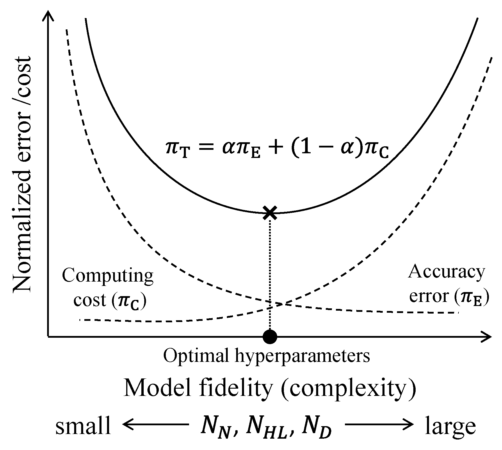
The PINN architecture shown in Figure 2 has three primary hyperparameters: the number of nodes ($N_{\mathrm{N}}$), the number of hidden layers ($N_{\mathrm{HL}}$) and the number of domains ($N_{\mathrm{D}}$). Here, $N_{\mathrm{N}}$ and $N_{\mathrm{HL}}$ account for the model complexity which enables capturing complicated physical behaviors embedded in the governing equation while $N_{\mathrm{D}}$ accounts for the amount of prior information provided by the governing equation. Therefore, these three primary hyperparameters determine the model fidelity of the PINN. As these hyperparameters increase, the model fidelity of the PINN improves meaning that the PINN predicts the solution of the governing equation more accurately and consistently. In contrast, the computing cost is likely to decrease as the hyperparameters decrease. In this regard, considering the trade-off between the accuracy error and computing cost, optimal hyperparameter combinations for the PINN should be determined. Figure 3 illustrates a schematic of determining optimal hyperparameter combinations considering this trade-off. The accuracy error monotonically decreases with the primary hyperparameters while the computing cost monotonically increases. By introducing a weight factor $\alpha$ that balances the importance of the solution accuracy and the computing cost, optimal hyperparameters can be determined so that the trade-off curve ${\pi }_{\mathrm{T}}$ is minimized.

3. Results and Discussion

3.1. Numerical Verification

3.1.1. Rectangular Cross Section

Figure 4 presents a 40 m long simply-supported PSC beam with a rectangular cross-section (width 0.6 m × height 1.2 m). The specification of the PSC beam is provided in

Table 1. Specification of the PSC beam in Figure 4.

Material Properties	Specification
$E_{\mathrm{ci}}$	33,600 MPa
$E_{\mathrm{p}}$	200 GPa
$A_{\mathrm{c}}$	0.72 m2
$I_{\mathrm{c}}$	0.0864 m4
$A_{\mathrm{p}}/A_{\mathrm{c}}$	1%
$e/h$	0.3
$f_{\mathrm{ck}}$	32 MPa
$f_{\mathrm{cu}}$	36 MPa
$f_{\mathrm{py}}$	1580 MPa
$f_{\mathrm{pi}}/f_{\mathrm{py}}$	0.7
$w_{\mathrm{c}}$	25 kN/m3

. Wet curing is conducted until $t_s=3\mathrm{days}$, after which shrinkage begins. The relative humidity of ambient environment RH = 70%. The PSC beam is post-tensioned to the initial prestressing force such that the initial prestressing ratio $f_{\mathrm{pi}}/f_{\mathrm{py}}=0.7$. It is assumed that the losses of prestressing force due to friction and anchorage draw-in have been taken into account in the initial prestressing ratio. The profile of the tendon is straight with a constant eccentricity ratio $e/h=0.3$. The time-dependent properties of concrete are calculated by using CEB-FIP Model Code 1990 [63]. The relaxation of the tendon is calculated by modifying the intrinsic stress relaxation function proposed by [64] for low-relaxation steel.

The forward finite difference method elaborated in Section 2.2.2 and Appendix A is adopted to obtain reference solutions of Equation (34). The analysis period is from $d_0=28\mathrm{days}$ on which the initial prestress transfer is carried out to 365 days, i.e., $0\le t\le 337$. Time increment $\mathsf{\Delta }t$ is 0.01685 day in the finite difference equation. The middle of the PSC beam is a section of interest for time-dependent analysis.

Table 2. Hyperparameter combinations of the PINN for solving Equation (34).

Hyperparameter	Combinations
$N_{\mathrm{N}}$	16, 32, 64, 128
$N_{\mathrm{NL}}$	5, 6, 7, 8
$N_D$	2, 4, 8, 16, 32, 64, 128, 256, 512
Activation function	elu
Optimizer	Adam + L-BFGS
Learning rate	0.001
Maximum iteration	10,000 for Adam optimizer
Number of Gauss quadrature points	40

presents hyperparameter combinations for varying $N_{\mathrm{N}}$, $N_{\mathrm{HL}}$ and $N_{\mathrm{D}}$ which are three primary hyperparameters described in Section 2.3.2. $N_{\mathrm{D}}$ is also known as the number of residual points. The residual points are randomly selected at the beginning of training and remain static during the training process. Once the residual points are selected, the deep neural networks are optimized to satisfy the physics imposed by the integro-differential governing equation at the selected residual points. A total of 144 combinations of primary hyperparameters are considered. The ‘elu’ activation function is adopted for the activation function and the Adam optimizer followed by L-BFGS is employed for optimization. Equation (36) is accurately approximated using 40 Gauss quadrature points. All computing simulations were conducted on a workstation equipped with an Intel Core i9-10900X CPU and an NVIDIA Quadro RTX 6000 GPU, running a Windows 10 Pro operating system. The DeepXDE [37] was adopted to implement the PINNs with hyperparameter combinations for solving Equation (34) in Table 2.

For each hyperparameter combination outlined in Table 2, accuracy errors are calculated through 30 times Monte-Carlo simulations to confirm the consistency of the predicted solutions. Here, the accuracy error is defined as the relative root mean square error between the predicted solution and the reference solution calculated from Equation (33). Figure 5 presents a box plot that exhibits the 16 mean values of the 30 accuracy errors, each corresponding to 1 of the 16 hyperparameter combinations per number of domains. The symbols ‘×’ and ‘o’ represent the mean values and the outliers of 16 mean values of the 30 accuracy errors, respectively. The median values in the box plot align closely with the mean values despite some outliers.

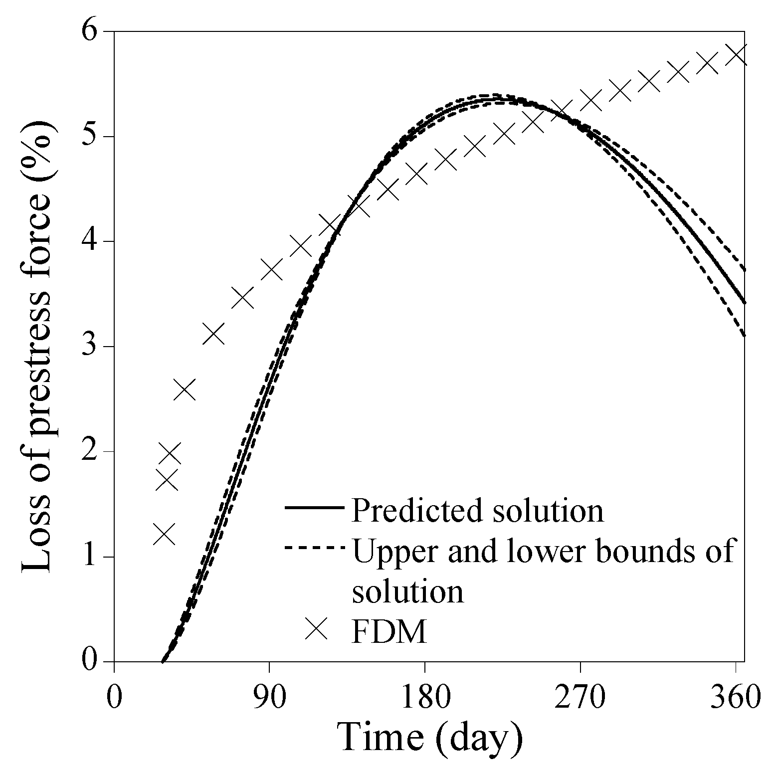
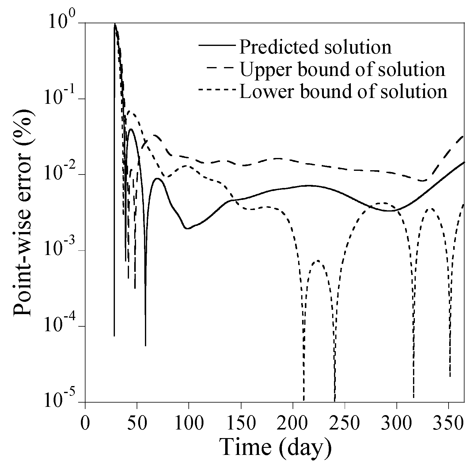
Three implications can be drawn from Figure 5. Firstly, the most critical hyperparameter is $N_{\mathrm{D}}$; the accuracy error decreases rapidly with $N_{\mathrm{D}}<32$ and then slows down with $N_{\mathrm{D}}\ge 32$. Secondly, when $N_{\mathrm{D}}$ is small, the accuracy error deviates to some extent with varying $N_{\mathrm{N}}$ and $N_{\mathrm{HL}}$. As $N_{\mathrm{D}}$ increases, however, the impact of $N_{\mathrm{N}}$ and $N_{\mathrm{HL}}$ on the accuracy error decreases quickly. Thirdly, when $N_{\mathrm{D}}$ is very small, the predicted solution from PINN is likely to poorly fit the reference solution as shown in Figure 6. In contrast, when $N_{\mathrm{D}}\ge 32$, the predicted solutions agree with the reference solution very well, as shown in Figure 7. The upper and lower bounds depicted in Figure 6 and Figure 7, which are set at a standard deviation away from the predicted solution, represent the solution precision for 30 times trials during the Monte-Carlo simulation. As observed in Figure 6, the solution precision is low when $N_{\mathrm{D}}$ is small, regardless of large $N_{\mathrm{N}}$ and $N_{\mathrm{HL}}$. Conversely, when $N_{\mathrm{D}}\ge 32$, the solution accuracy improves significantly for the identical $N_{\mathrm{N}}$ and $N_{\mathrm{HL}}$, as shown in Figure 7. The point-wise errors of the well-fitted results from PINN in Figure 7 are presented in Figure 8.

Similar to Figure 5, Figure 9 illustrates a box plot that provides the mean values of the 30 computing times, each corresponding to 1 of the 16 hyperparameter combinations per number of domains. Similar to Figure 5, the median values in the box plot are almost identical to the mean values, though some outliers are observed. The computing time increases monotonically as $N_{\mathrm{D}}$ increases. Up to $N_{\mathrm{D}}=64$, the computation time remains constant regardless of $N_{\mathrm{N}}$ and $N_{\mathrm{HL}}$, while for $N_{\mathrm{D}}\ge 128$, the computation time increases with $N_{\mathrm{N}}$ and $N_{\mathrm{HL}}$.

The optimal $N_{\mathrm{D}}$ is determined by using the trade-off curve between accuracy error and computing cost in Figure 3. The accuracy error ${\pi }_{\mathrm{E}}$ and the computing cost ${\pi }_{\mathrm{C}}$ in Figure 3 are calculated with respect to $N_{\mathrm{D}}$ by using the associated mean values in Figure 5 and Figure 9, respectively. Note that the mean values in Figure 5 and Figure 9 are normalized, respectively, so that the maximum values of ${\pi }_{\mathrm{E}}$ and ${\pi }_{\mathrm{C}}$ become unit values. Figure 10 illustrates trade-off curves to determine an optimal hyperparameter $N_{\mathrm{D}}$ for three different weight factors $\alpha =0.5,0.7$ and $0.8$. When $\alpha =0.5$, the solution accuracy and the computing cost are equally important, while the solution accuracy is four times more important than the computing cost when $\alpha =0.8$. Observing Figure 10, the optimal $N_{\mathrm{D}}$ corresponds to 16, 32, and 64 for $\alpha =0.5,0.7,$ and $0.8$, respectively.

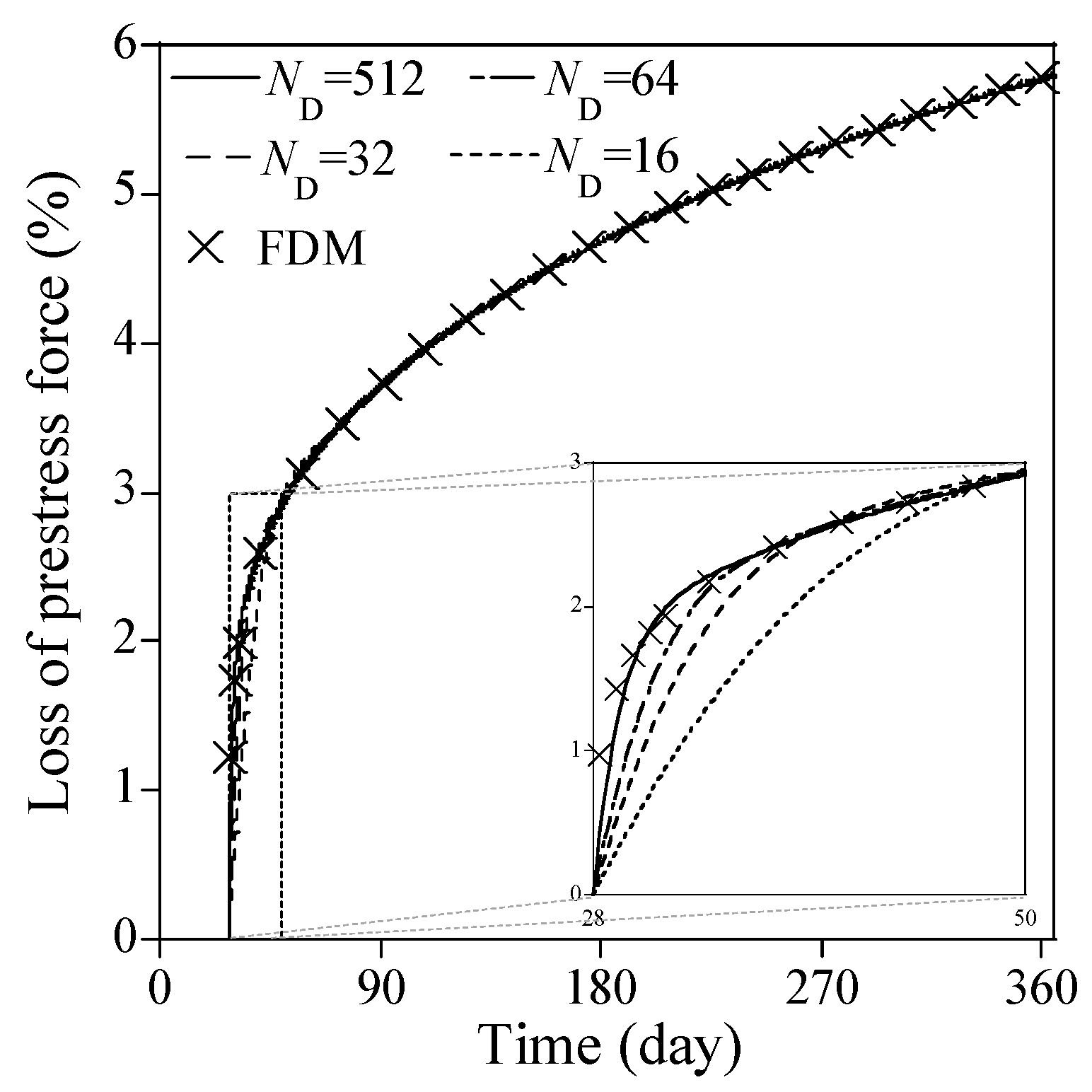
Figure 11 presents the predicted solutions from Equation (34) for $N_{\mathrm{D}}=16$, 32, and 64, respectively, with $N_{\mathrm{N}}=64$ and $N_{\mathrm{HL}}=8$. Note that each predicted solution is the mean of 30 solutions from the Monte-Carlo simulation for each combination of $N_{\mathrm{D}}$, $N_{\mathrm{N}}$ and $N_{\mathrm{HL}}$. For comparison purposes, the predicted solution corresponding to $N_{\mathrm{D}}=512$, $N_{\mathrm{N}}=128$ and $N_{\mathrm{HL}}=8$ is presented as standing for the most accurate solution available from the PINN, while the numerical solution from the finite difference method is provided as the reference solution. Overall, the three predicted solutions for $N_{\mathrm{D}}=16$, 32, and 64 agree very well with that for $N_{\mathrm{D}}=512$, and the reference solution after 60 days, though there exist slight differences from 28 days to 50 days. As $N_{\mathrm{D}}$ increases, these differences vanish, as shown at the right bottom in Figure 11. The corresponding point-wise errors from 28 days to 50 days are presented in Figure 12.

Based on the observation of Figure 10 and Figure 11, the optimal combinations of the primary hyperparameters in the PINNs are determined as $N_{\mathrm{D}}=32$, $N_{\mathrm{N}}=64$ and $N_{\mathrm{HL}}=8$. Note that the number of nodes ($N_{\mathrm{N}}$) and the number of hidden layers ($N_{\mathrm{HL}}$) affect neither the accuracy error nor the computation time when $N_{\mathrm{D}}=$ 32. Therefore, this hyperparameter combination is adopted in PINNs to solve Equation (34) throughout the numerical verification otherwise mentioned hereafter.

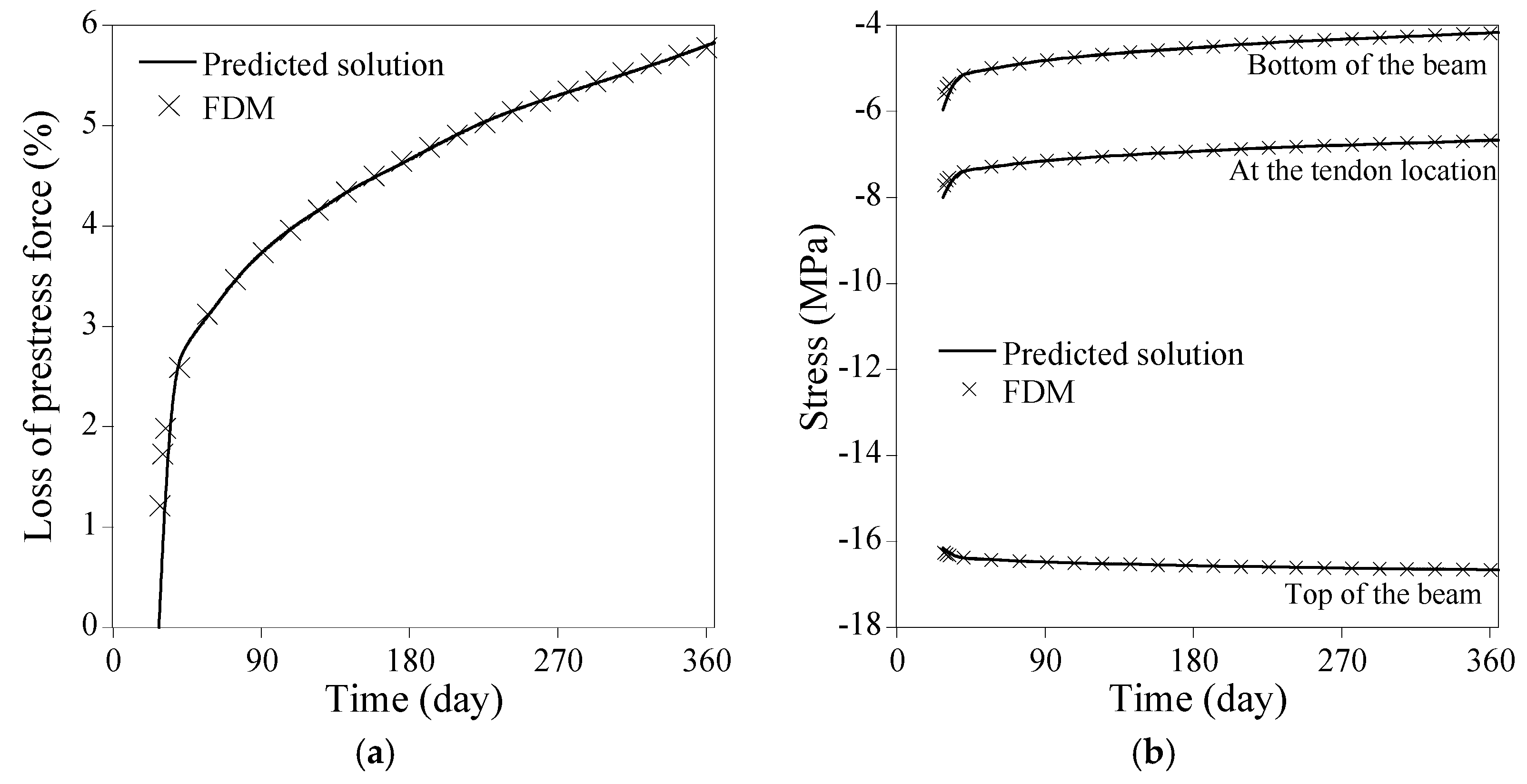
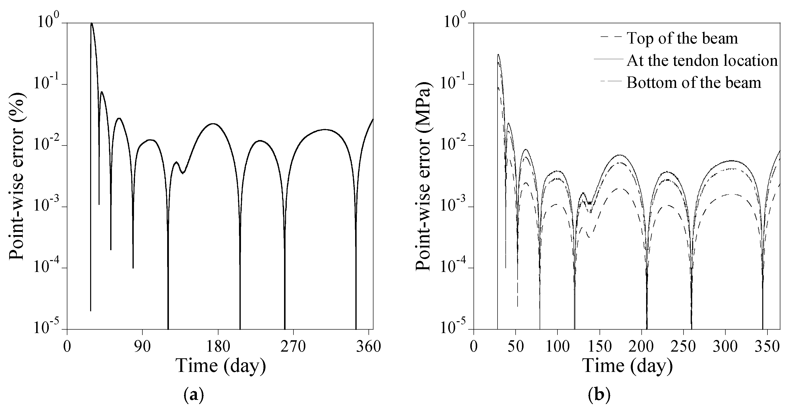
Figure 13a shows the comparison of the numerical results from the proposed PINN to the forward finite difference method regarding the loss of prestress force in case all time-dependent factors of the PSC beam are accounted for. The full coupling among the elastic modulus, creep and shrinkage of concrete, and the relaxation of tendon affects loss of prestress force with time. The loss of prestress force surges to 3.7% at 90 days and approaches 5.8% at 365 days. Figure 13b compares the stresses at the top and the bottom of the beam and at the tendon location. The final fractional magnitudes of the stresses at the top and the bottom of the beam, and at the tendon location become 103%, 83.3%, and 69.8%, respectively, compared to those on 28 days. The point-wise errors of the numerical results from the PINNs in Figure 13 are presented in Figure 14. The proposed method yields satisfactory results compared to the forward finite difference method. The absolute difference at 365 days in loss of prestress force is 0.027%, while that in all stresses at the top and the bottom of the beam and the tendon location is less than 0.20%.

3.1.2. Conventional PSC I-Beam Section

Figure 15 presents a 45 m long simply-supported PSC beam with an I-shaped cross section. The specification of the PSC beam is provided in

Table 3. Specification of the PSC I-beam in Figure 15.

Material Properties	Specification
$E_{\mathrm{ci}}$	35,385 MPa
$E_{\mathrm{p}}$	200 GPa
$A_{\mathrm{c}}$	1.084 m2
$I_{\mathrm{c}}$	0.6454 m4
$A_{\mathrm{p}}/A_{\mathrm{c}}$	0.972%
$e/h$	0.445
$f_{\mathrm{ck}}$	40 MPa
$f_{\mathrm{cu}}$	44 MPa
$f_{\mathrm{py}}$	1580 MPa
$f_{\mathrm{pi}}/f_{\mathrm{py}}$	0.7
$w_{\mathrm{c}}$	25 kN/m3

. All design parameters not present in Table 3 are identical to those in Section 3.1.1 except for the tendon profile, which is parabolic with a maximum eccentricity ratio $e/h=0.445$ at the middle of the beam.

The analysis of time-dependent behaviors of the PSC beam is conducted by using the forward finite difference method in the same way described in Section 3.1.1 to obtain the reference solution. The analysis period is from the $d_0=7\mathrm{days}$ on which the initial prestress transfer is conducted to 365 days, i.e., $0\le t\le 358$. The time increment $\mathsf{\Delta }t$ is 0.01685 days in the finite difference equation. The middle of the PSC beam is a section of interest for time-dependent analysis. The optimal combination of the primary hyperparameters in the PINNs is identical to that used in Section 3.1.1: $N_{\mathrm{N}}=64$, $N_{\mathrm{HL}}=8$, $N_{\mathrm{D}}=32$.

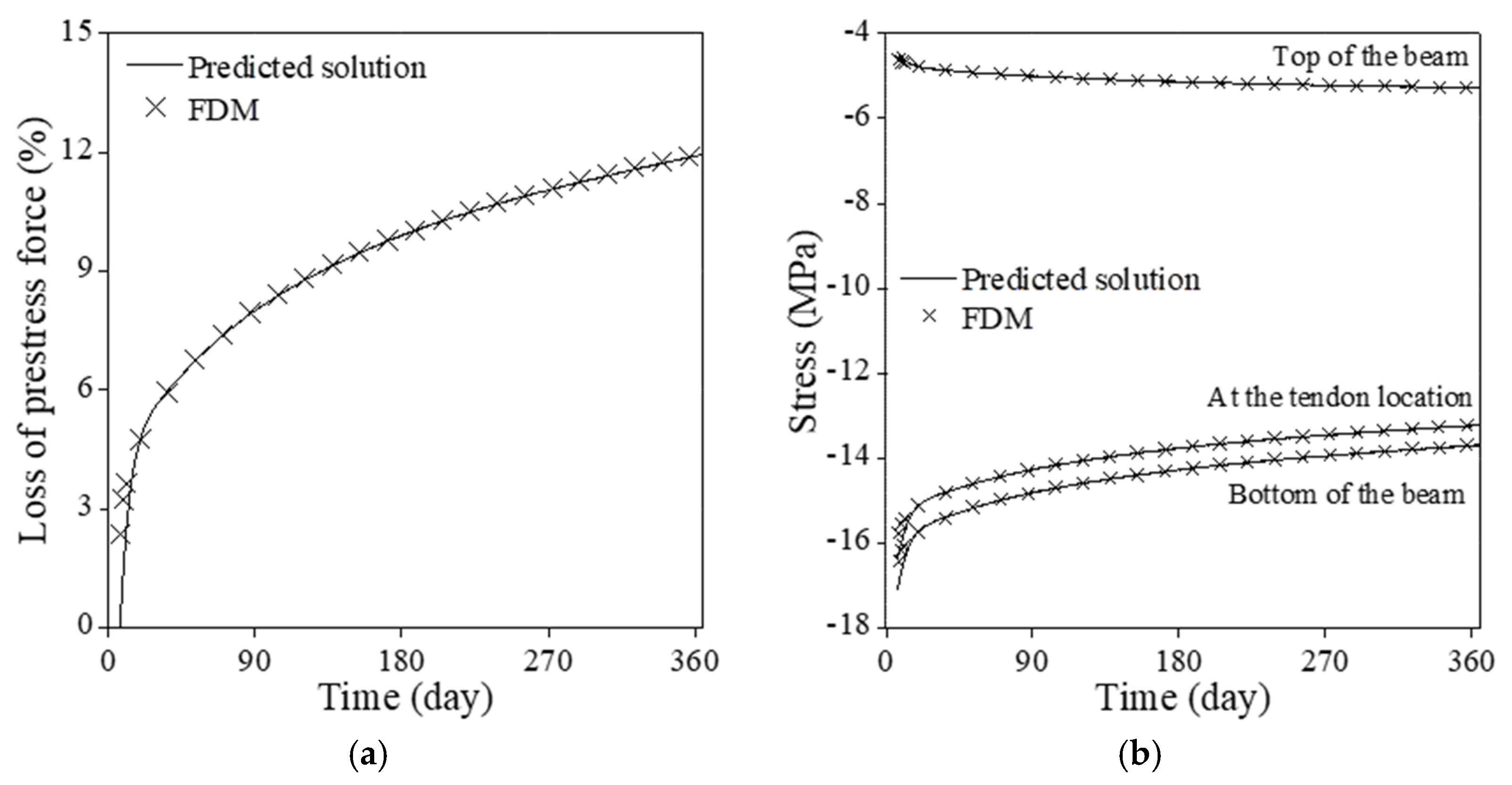
Figure 16a illustrates the comparison between the proposed PINNs and the forward finite difference method for loss of prestress force considering all time-dependent factors of the PSC beam. The complete interaction among the elastic modulus, concrete creep and shrinkage, and tendon relaxation influences the prestress loss over time. The loss of prestress force surges to 8.0% at 90 days and reaches 12% at 365 days. Figure 16b contrasts the stress levels at the beam’s top, bottom, and tendon locations. The final fractional stress magnitudes at these locations are 119%, 80.6%, and 80.0%, respectively, compared to those on 28 days. The point-wise errors of the numerical results from the PINNs in Figure 16 are presented in Figure 17. The proposed method yields satisfactory outcomes when compared to the forward finite difference method. The absolute difference at 365 days in prestress force loss is 0.042% while that in all stresses at the top and the bottom of the beam and the tendon location remains below 0.0075%.

4. Conclusions

In this study, a PINN approach was proposed to predict the early-age time-dependent behaviors of the PSC beam. The original contributions of this study are presented below:

• The dimensionless integro-differential governing equation is derived for the PINN. The governing equation accounts for time-dependent coupling among the effective prestress force and several factors including concrete creep and shrinkage, tendon relaxation, and changes in concrete elastic modulus.
• The fidelity of the PINN is determined by three primary hyperparameters: the number of nodes, the number of hidden layers, and the number of domains. Among these primary hyperparameters, the number of domains is the most critical factor for the accuracy and consistency of predicted solutions from the PINN. Optimal hyperparameter combinations for the PINN were determined by considering the trade-off between solution accuracy and computation time.
• The numerical results from the PINN with an optimal hyperparameter combination yielded satisfactory results, with absolute differences at 365 days in loss of prestress force being 0.027% and in all stresses at the top and bottom of the beam and the tendon location being less than 0.2% for PSC beams with a rectangular and an I-shaped section.
• The proposed PINN approach can effectively predict time-dependent behaviors of PSC beams, offering a promising alternative to conventional numerical methods. The proposed PINN can address the limitations of conventional machine learning by training deep neural networks that satisfy the governing equation associated with the complicated time-dependent behaviors of the PSC beam.

Future work will pursue a PINN to solve inverse problems such as estimating time-dependent material properties related to the concrete creep and shrinkage, and the relaxation of the tendon by using a limited amount of actual measurement data from the PSC beam. It is necessary to implement a more advanced PINN to solve the proposed integro-differential equation to improve the performance of the conventional PINN used in the present study. Future work will explore the incorporation of optimal adaptive activation functions [43,44,45,46], which could further improve its accuracy and convergence.

References

1. Raissi, M.; Perdikaris, P.; Karniadakis, G.E. Physics informed deep learning (Part I): Data-driven solutions of nonlinear partial differential equations. arXiv 2017, arXiv:1711.10561. [Google Scholar]
2. Raissi, M.; Perdikaris, P.; Karniadakis, G.E. Physics informed deep learning (Part II): Data-driven discovery of nonlinear partial differential equations. arXiv 2017, arXiv:1711.10566. [Google Scholar]
3. Fujita, K. Physics-informed neural network method for modelling beam-wall interactions. Electron. Lett. 2022, 58, 390–392. [Google Scholar] [CrossRef]
4. Tartakovsky, A.M.; Marrero, C.O.; Perdikaris, P.; Tartakovsky, G.D.; Barajas-Solano, D. Learning parameters and constitutive relationships with physics informed deep neural networks. arXiv 2018, arXiv:1808.03398. [Google Scholar]
5. Raissi, M.; Perdikaris, P.; Karniadakis, G.E. Physics-informed neural networks: A deep learning framework for solving forward and inverse problems involving nonlinear partial differential equations. J. Comput. Phys. 2019, 378, 686–707. [Google Scholar] [CrossRef]
6. Raissi, M.; Yazdani, A.; Karniadakis, G.E. Hidden fluid mechanics: Learning velocity and pressure fields from flow visualizations. Science 2020, 367, 1026–1030. [Google Scholar] [CrossRef]
7. He, Q.; Barajas-Solano, D.; Tartakovsky, G.; Tartakovsky, A.M. Physics-informed neural networks for multi-physics data assimilation with application to subsurface transport. Adv. Water Resour. 2020, 141, 103610. [Google Scholar] [CrossRef]
8. Karimpouli, S.; Tahmasebi, P. Physics informed machine learning: Seismic wave equation. Geosci. Front. 2020, 11, 1993–2001. [Google Scholar] [CrossRef]
9. Yang, L.; Meng, X.; Karniadakis, G.E. B-PINNs: Bayesian physics-informed neural networks for forward and inverse PDE problems with noisy data. J. Comput. Phys. 2021, 425, 109913. [Google Scholar] [CrossRef]
10. Jagtap, A.D.; Kharazmi, E.; Karniadakis, G.E. Conservative physics-informed neural networks on discrete domains for conservation laws: Applications to forward and inverse problems. Comput. Methods Appl. Mech. Eng. 2020, 365, 113028. [Google Scholar] [CrossRef]
11. Yucesan, Y.A.; Viana, F.A. Wind turbine main bearing fatigue life estimation with physics-informed neural networks. In Proceedings of the Annual Conference of the PHM Society, Scottsdale, AZ, USA, 21–26 September 2019; Volume 11, pp. 1–14. [Google Scholar]
12. Chen, Y.; Lu, L.; Karniadakis, G.E.; Dal Negro, L. Physics-informed neural networks for inverse problems in nano-optics and metamaterials. Opt. Express 2020, 28, 11618–11633. [Google Scholar] [CrossRef] [PubMed] [Green Version]
13. Goswami, S.; Anitescu, C.; Chakraborty, S.; Rabczuk, T. Transfer learning enhanced physics informed neural network for phase-field modeling of fracture. Theor. Appl. Fract. Mech. 2020, 106, 102447. [Google Scholar] [CrossRef] [Green Version]
14. Kadeethum, T.; Jørgensen, T.M.; Nick, H.M. Physics-informed neural networks for solving nonlinear diffusivity and Biot’s equations. PLoS ONE 2020, 15, e0232683. [Google Scholar] [CrossRef] [PubMed]
15. Tartakovsky, A.M.; Marrero, C.O.; Perdikaris, P.; Tartakovsky, G.D.; Barajas-Solano, D. Physics-informed deep neural networks for learning parameters and constitutive relationships in subsurface flow problems. Water Resour. Res. 2020, 56, e2019WR026731. [Google Scholar] [CrossRef]
16. Mao, Z.; Jagtap, A.D.; Karniadakis, G.E. Physics-informed neural networks for high-speed flows. Comput. Methods Appl. Mech. Eng. 2020, 360, 112789. [Google Scholar] [CrossRef]
17. Jin, X.; Cai, S.; Li, H.; Karniadakis, G.E. NSFnets (Navier-Stokes flow nets): Physics-informed neural networks for the incompressible Navier-Stokes equations. J. Comput. Phys. 2021, 426, 109951. [Google Scholar] [CrossRef]
18. Jagtap, A.D.; Mao, Z.; Adams, N.; Karniadakis, G.E. Physics-informed neural networks for inverse problems in supersonic flows. J. Comput. Phys. 2022, 466, 111402. [Google Scholar] [CrossRef]
19. Kissas, G.; Yang, Y.; Hwuang, E.; Witschey, W.R.; Detre, J.A.; Perdikaris, P. Machine learning in cardio-vascular flows modeling: Predicting arterial blood pressure from non-invasive 4D flow MRI data using physics-informed neural networks. Comput. Methods Appl. Mech. Eng. 2020, 358, 112623. [Google Scholar] [CrossRef]
20. Haghighat, E.; Raissi, M.; Moure, A.; Gomez, H.; Juanes, R. A deep learning framework for solution and discovery in solid mechanics. arXiv 2020, arXiv:2003.02751. [Google Scholar]
21. Rao, C.; Sun, H.; Liu, Y. Physics-informed deep learning for computational elastodynamics without labeled data. J. Eng. Mech. 2021, 147, 04021043. [Google Scholar] [CrossRef]
22. Alkhadhr, S.; Almekkawy, M. Wave equation modeling via physics-informed neural networks: Models of soft and hard constraints for initial and boundary conditions. Sensors 2023, 23, 2792. [Google Scholar] [CrossRef]
23. Tarkhov, D.; Lazovskaya, T.; Malykhina, G. Constructing physics-informed neural networks with architecture based on analytical modification of numerical methods by solving the problem of modelling processes in a chemical reactor. Sensors 2023, 23, 663. [Google Scholar] [CrossRef] [PubMed]
24. Boushaba, A.; Cauet, S.; Chamroo, A.; Etien, E.; Rambault, L. Comparative study between physics-informed CNN and PCA in induction motor broken bars MCSA detection. Sensors 2022, 22, 9494. [Google Scholar] [CrossRef] [PubMed]
25. Shukla, K.; Jagtap, A.D.; Blackshire, J.L.; Sparkman, D.; Karniadakis, G.E. A physics-informed neural network for quantifying the microstructural properties of polycrystalline nickel using ultrasound data: A promising approach for solving inverse problems. IEEE Signal Process. Mag. 2021, 39, 68–77. [Google Scholar] [CrossRef]
26. Jagtap, A.D.; Mitsotakis, D.; Karniadakis, G.E. Deep learning of inverse water waves problems using multi-fidelity data: Application to Serre–Green–Naghdi equations. Ocean Eng. 2022, 248, 110775. [Google Scholar] [CrossRef]
27. Yuan, L.; Ni, Y.Q.; Deng, X.Y.; Hao, S. A-PINN: Auxiliary physics informed neural networks for forward and inverse problems of nonlinear integro-differential equations. J. Comput. Phys. 2022, 462, 111260. [Google Scholar] [CrossRef]
28. Pang, G.; Lu, L.; Karniadakis, G.E. fPINNs: Fractional physics-informed neural networks. SIAM J. Sci. Comput. 2019, 41, A2603–A2626. [Google Scholar] [CrossRef] [Green Version]
29. Nabian, M.A.; Meidani, H. A deep neural network surrogate for high-dimensional random partial differential equations. arXiv 2018, arXiv:1806.02957. [Google Scholar]
30. Zhang, D.; Lu, L.; Guo, L.; Karniadakis, G.E. Quantifying total uncertainty in physics-informed neural networks for solving forward and inverse stochastic problems. J. Comput. Phys. 2019, 397, 108850. [Google Scholar] [CrossRef] [Green Version]
31. Yang, L.; Zhang, D.; Karniadakis, G.E. Physics-informed generative adversarial networks for stochastic differential equations. SIAM J. Sci. Comput. 2020, 42, A292–A317. [Google Scholar] [CrossRef] [Green Version]
32. Zhang, D.; Guo, L.; Karniadakis, G.E. Learning in modal space: Solving time-dependent stochastic PDEs using physics-informed neural networks. SIAM J. Sci. Comput. 2020, 42, A639–A665. [Google Scholar] [CrossRef]
33. Mishra, S.; Molinaro, R. Estimates on the generalization error of physics-informed neural networks for approximating a class of inverse problems for PDEs. IMA J. Numer. Anal. 2022, 42, 981–1022. [Google Scholar] [CrossRef]
34. Hu, Z.; Jagtap, A.D.; Karniadakis, G.E.; Kawaguchi, K. When do extended physics-informed neural networks (XPINNs) improve generalization? SIAM J. Sci. Comput. 2022, 44, A3158–A3182. [Google Scholar] [CrossRef]
35. De Ryck, T.; Jagtap, A.D.; Mishra, S. Error estimates for physics-informed neural networks approximating the Navier–Stokes equations. IMA J. Numer. Anal. 2023, drac085. [Google Scholar] [CrossRef]
36. Karniadakis, G.E.; Kevrekidis, I.G.; Lu, L.; Perdikaris, P.; Wang, S.; Yang, L. Physics-informed machine learning. Nat. Rev. Phys. 2021, 3, 422–440. [Google Scholar] [CrossRef]
37. Lu, L.; Meng, X.; Mao, Z.; Karniadakis, G.E. DeepXDE: A deep learning library for solving differential equations. SIAM Rev. 2021, 63, 208–228. [Google Scholar] [CrossRef]
38. Amini, D.; Haghighat, E.; Juanes, R. Physics-informed neural network solution of thermo–hydro–mechanical processes in porous media. J. Eng. Mech. 2022, 148, 04022070. [Google Scholar] [CrossRef]
39. Jagtap, A.D.; Karniadakis, G.E. Extended Physics-Informed Neural Networks (XPINNs): A generalized space-time domain decomposition based deep learning framework for nonlinear partial differential equations. Commun. Comput. Phys. 2020, 28, 2002–2041. [Google Scholar]
40. Shukla, K.; Jagtap, A.D.; Karniadakis, G.E. Parallel physics-informed neural networks via domain decomposition. J. Comput. Phys. 2021, 447, 110683. [Google Scholar] [CrossRef]
41. Hu, Z.; Jagtap, A.D.; Karniadakis, G.E.; Kawaguchi, K. Augmented physics-informed neural networks (APINNs): A gating network-based soft domain decomposition methodology. arXiv 2022, arXiv:2211.08939. [Google Scholar]
42. Penwarden, M.; Jagtap, A.D.; Zhe, S.; Karniadakis, G.E.; Kirby, R.M. A unified scalable framework for causal sweeping strategies for Physics-Informed Neural Networks (PINNs) and their temporal decompositions. arXiv 2023, arXiv:2302.14227. [Google Scholar]
43. Jagtap, A.D.; Kawaguchi, K.; Karniadakis, G.E. Adaptive activation functions accelerate convergence in deep and physics-informed neural networks. J. Comput. Phys. 2020, 404, 109136. [Google Scholar] [CrossRef] [Green Version]
44. Jagtap, A.D.; Kawaguchi, K.; Em Karniadakis, G. Locally adaptive activation functions with slope recovery for deep and physics-informed neural networks. Proc. R. Soc. A 2020, 476, 20200334. [Google Scholar] [CrossRef]
45. Jagtap, A.D.; Shin, Y.; Kawaguchi, K.; Karniadakis, G.E. Deep Kronecker neural networks: A general framework for neural networks with adaptive activation functions. Neurocomputing 2022, 468, 165–180. [Google Scholar] [CrossRef]
46. Jagtap, A.D.; Karniadakis, G.E. How important are activation functions in regression and classification? A survey, performance comparison, and future directions. arXiv 2022, arXiv:2209.02681. [Google Scholar] [CrossRef]
47. Maroliya, M.K. Comparative study of flexural behavior of reinforced concrete beam and prestressed concrete beam. Int. J. Eng. Res. Appl. (IJERA) 2012, 2, 230–233. [Google Scholar]
48. Porco, F.; Fiore, A.; Porco, G.; Uva, G. Monitoring and safety for prestressed bridge girders by SOFO sensors. J. Civ. Struct. Health Monit. 2013, 3, 3–18. [Google Scholar] [CrossRef]
49. Garber, D.B.; Gallardo, J.M.; Deschenes, D.J.; Bayrak, O. Experimental investigation of prestress losses in full-scale bridge girders. ACI Struct. J. 2015, 112, 553–564. [Google Scholar] [CrossRef] [Green Version]
50. Butler, L.J.; Gibbons, N.; He, P.; Middleton, C.; Elshafie, M.Z. Evaluating the early-age behaviour of full-scale prestressed concrete beams using distributed and discrete fibre optic sensors. Constr. Build. Mater. 2016, 126, 894–912. [Google Scholar] [CrossRef]
51. Yang, I.H. Uncertainty and sensitivity analysis of time-dependent effects in concrete structures. Eng. Struct. 2007, 29, 1366–1374. [Google Scholar] [CrossRef]
52. Caro, L.A.; Martí-Vargas, J.R.; Serna, P. Time-dependent evolution of strand transfer length in pretensioned prestressed concrete members. Mech. Time-Depend. Mater. 2013, 17, 501–527. [Google Scholar] [CrossRef]
53. Ranzi, G.; Al-Deen, S.; Ambrogi, L.; Uy, B. Long-term behaviour of simply-supported post-tensioned composite slabs. J. Constr. Steel Res. 2013, 88, 172–180. [Google Scholar] [CrossRef]
54. Li, D.; Kaewunruen, S. Effect of extreme climate on topology of railway prestressed concrete sleepers. Climate 2019, 7, 17. [Google Scholar] [CrossRef] [Green Version]
55. Zawam, M.; Soudki, K.; West, J.S. Factors affecting the time-dependent behaviour of GFRP prestressed concrete beams. J. Build. Eng. 2019, 24, 100715. [Google Scholar] [CrossRef]
56. Joyklad, P.; Ali, N.; Chaiyasarn, K.; Suparp, S.; Hussain, Q. Time-dependent behavior of full-scale precast post-tensioned (PCPT) girders: Experimental and finite element analysis. Case Stud. Constr. Mater. 2022, 17, e01310. [Google Scholar] [CrossRef]
57. Robertson, I.N. Prediction of vertical deflections for a long-span prestressed concrete bridge structure. Eng. Struct. 2005, 27, 1820–1827. [Google Scholar] [CrossRef]
58. Au, F.T.; Si, X.T. Accurate time-dependent analysis of concrete bridges considering concrete creep, concrete shrinkage and cable relaxation. Eng. Struct. 2011, 33, 118–126. [Google Scholar] [CrossRef]
59. Lou, T.; Karavasilis, T.L. Time-dependent assessment and deflection prediction of prestressed concrete beams with unbonded CFRP tendons. Compos. Struct. 2018, 194, 365–376. [Google Scholar] [CrossRef] [Green Version]
60. Páez, P.M.; Sensale, B. Improved prediction of long-term prestress loss in unbonded prestressed concrete members. Eng. Struct. 2018, 174, 111–125. [Google Scholar] [CrossRef]
61. Gilbert, R.I.; Mickleborough, N.C. Design of Prestressed Concrete; CRC Press: Boca Raton, FL, USA, 1990. [Google Scholar]
62. Liu, R.; Ye, H.; Liu, Y.; Zhao, H.; Correia, J.A.; Xin, H. Numerical simulation of concrete creep behaviour using integral creep algorithm with alternating stresses. Structures 2021, 29, 1979–1987. [Google Scholar] [CrossRef]
63. Comité Euro-International du Béton. CEB-FIP Model Code 1990: Design Code; Thomas Telford: London, UK, 1993. [Google Scholar]
64. Magura, D.D.; Sozen, M.A.; Siess, C.P. A study of stress relaxation in prestressing reinforcement. Civ. Eng. Stud. SRS-237 1962. [Google Scholar] [CrossRef]
Figure 2. The basic architecture of the PINN.
Sensors 23 06649 g002
Figure 3. Schematic of determining optimal hyperparameters for the PINN using a trade-off curve ( π T ) between accuracy error and computing cost where π T = α π E + 1 α π C and 0 α 1 .
Sensors 23 06649 g003
Figure 4. A 40 m long simply-supported PSC beam with a rectangular cross section.
Sensors 23 06649 g004
Figure 5. Accuracy error of PINN for solving Equation (34). ‘×’ and ‘o’ represent mean values and outliers, respectively.
Sensors 23 06649 g005
Figure 6. Poorly fitted results from PINN for solving Equation (34) [ N N = 128 , N HL = 7 , N D = 2 ].
Sensors 23 06649 g006
Figure 7. Well-fitted results from PINN for solving Equation (34) [ N N = 128 , N HL = 7 , N D = 32 ].
Sensors 23 06649 g007
Figure 8. Point-wise errors of the well-fitted results from PINN in Figure 7.
Sensors 23 06649 g008
Figure 9. Computing time of PINN for solving Equation (34). ‘×’ and ‘o’ represent mean values and outliers, respectively.
Sensors 23 06649 g009
Figure 10. Determining optimal N D through trade-off curves for different α as described in Figure 3.
Sensors 23 06649 g010
Figure 11. The predicted solutions using optimal N D for different α from Figure 10 with N N = 64 and N HL = 8 .
Sensors 23 06649 g011
Figure 12. Point-wise errors of the predicted solutions from 28 days to 50 days as in Figure 11.
Sensors 23 06649 g012
Figure 13. Comparison of numerical results from the PINNs ( N N = 64 , N HL = 8 , N D = 32 ) to the forward finite difference method: (a) loss of prestress force; (b) stress at the top and the bottom of the beam and at the tendon location.
Sensors 23 06649 g013
Figure 14. Point-wise error of the numerical results from the PINNs in Figure 13: (a) loss of prestress force; (b) stress at the top and the bottom of the beam and at the tendon location.
Sensors 23 06649 g014
Figure 15. A 45 m long simply-supported PSC beam with an I-shaped cross section.
Sensors 23 06649 g015
Figure 16. Comparison of numerical results from PINNs ( N N = 64 , N HL = 8 , N D = 32 ) to the forward finite difference method: (a) loss of prestress force; (b) stress at the top and the bottom of the beam and at the tendon location.
Sensors 23 06649 g016
Figure 17. Point-wise error of the numerical results from the PINNs in Figure 16: (a) loss of prestress force; (b) stress at the top and the bottom of the beam and at the tendon location.
Sensors 23 06649 g017