

Predicting Rice Lodging Risk from the Distribution of Available Nitrogen in Soil Using UAS Images in a Paddy Field

 ,
,  and
and 
Abstract
1. Introduction
2. Methods
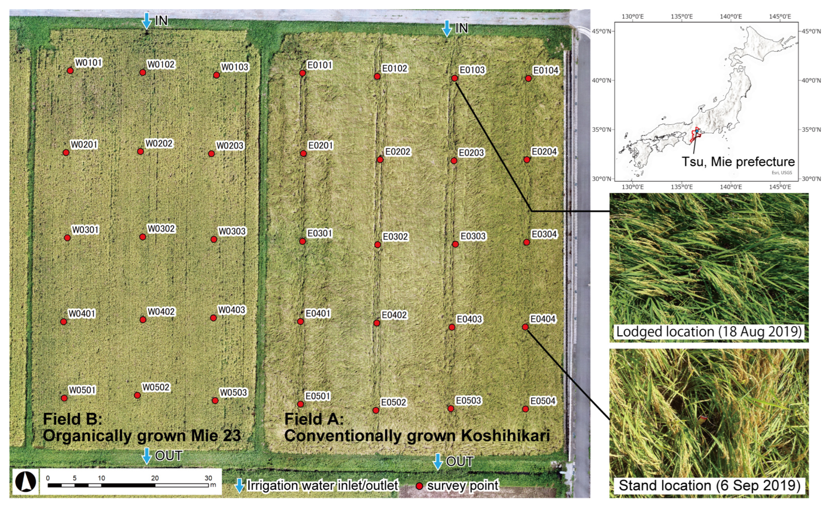
2.1. Field Survey
2.1.1. Study Field
2.1.2. Rice Growth Survey
2.1.3. Soil Sampling and Chemical Properties
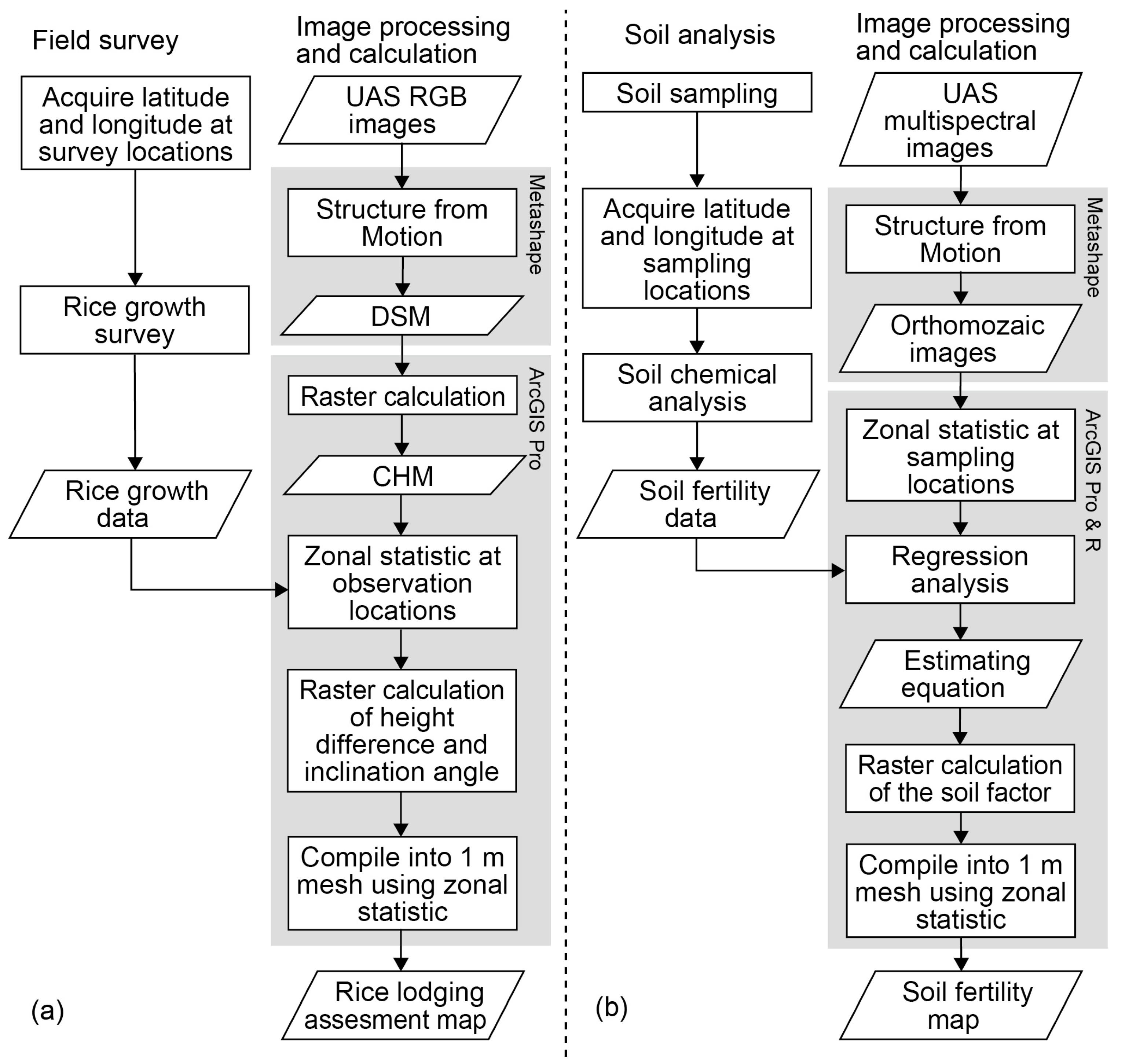
2.2. Image Processing and Analysis
2.2.1. UAS Platform
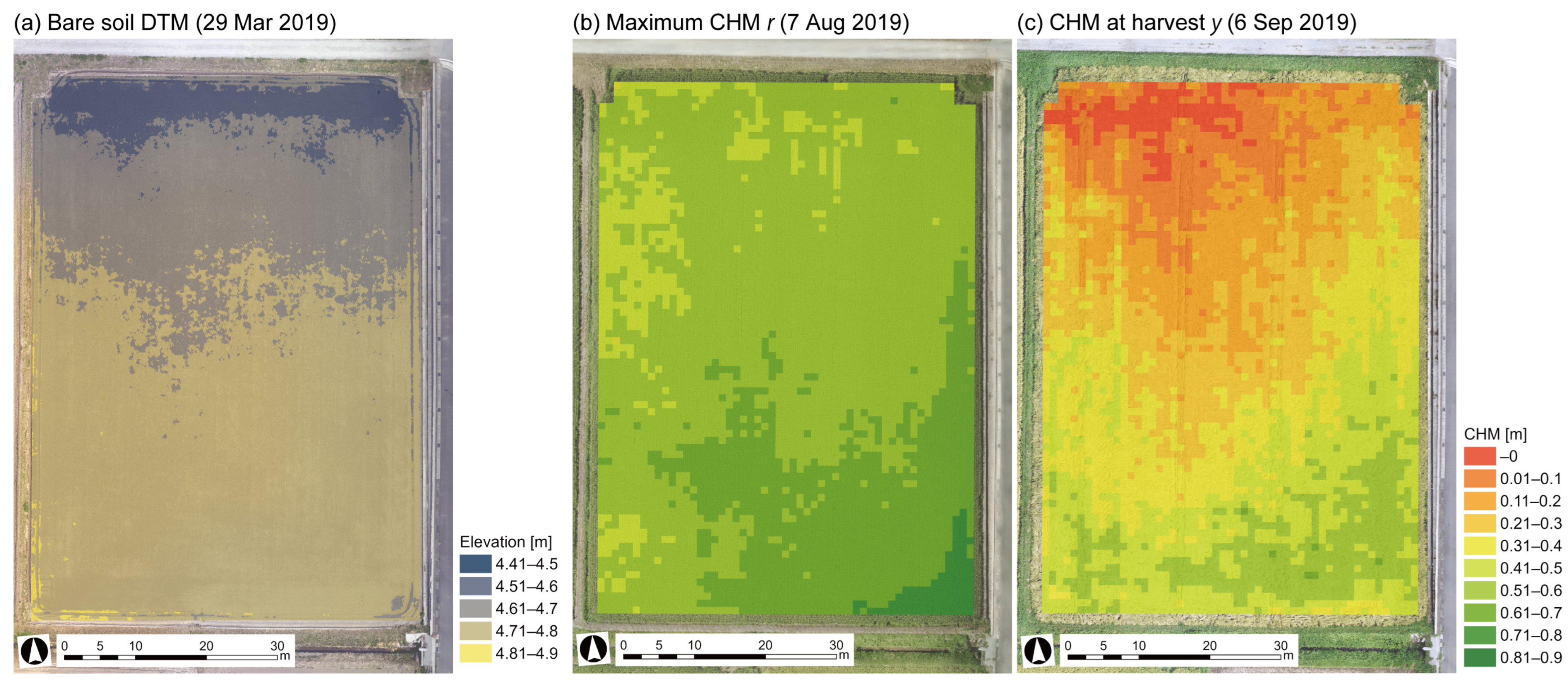
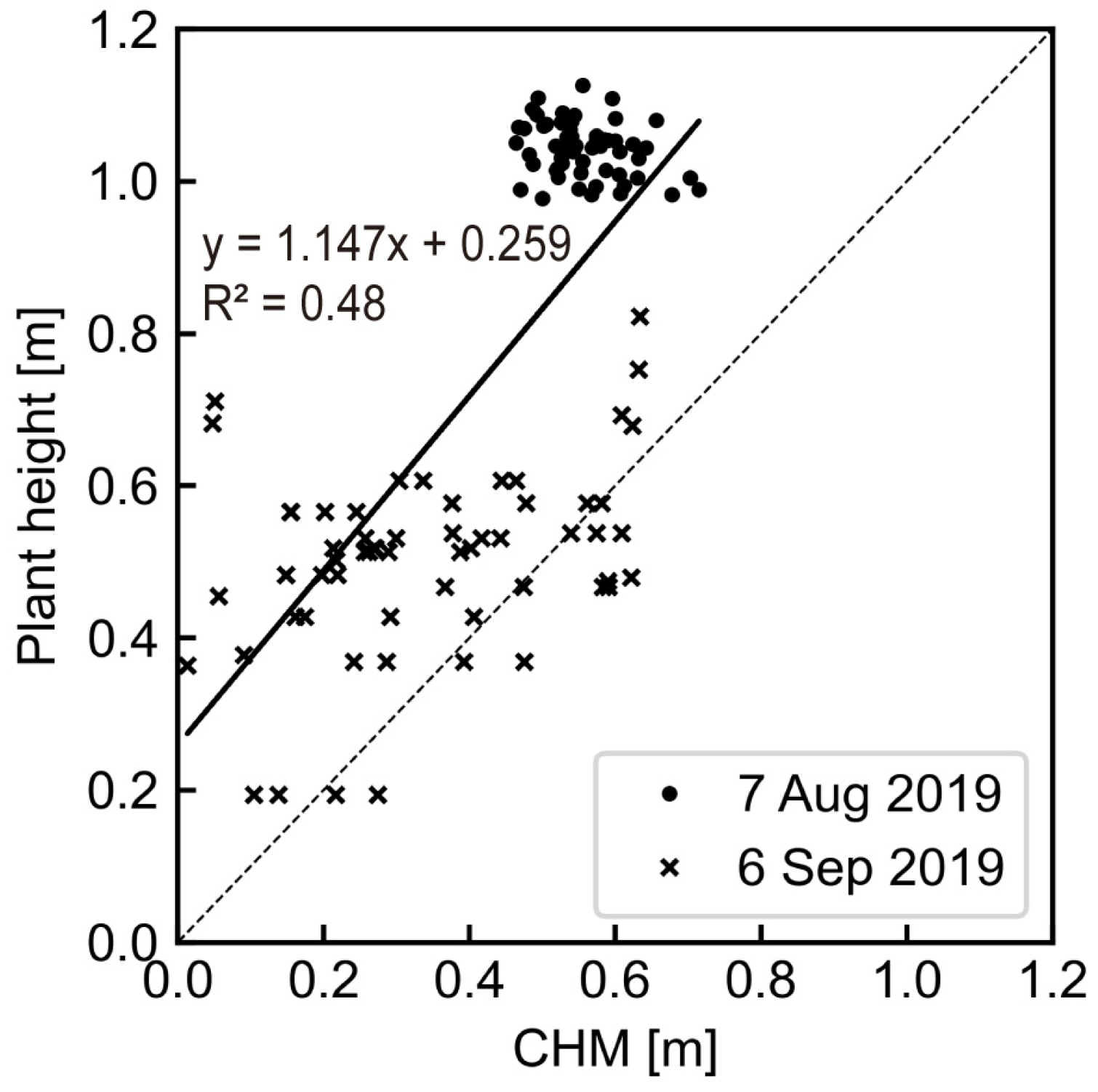
2.2.2. Assessment of Rice Growth and Lodging
2.2.3. Estimate of Soil Fertility
3. Results
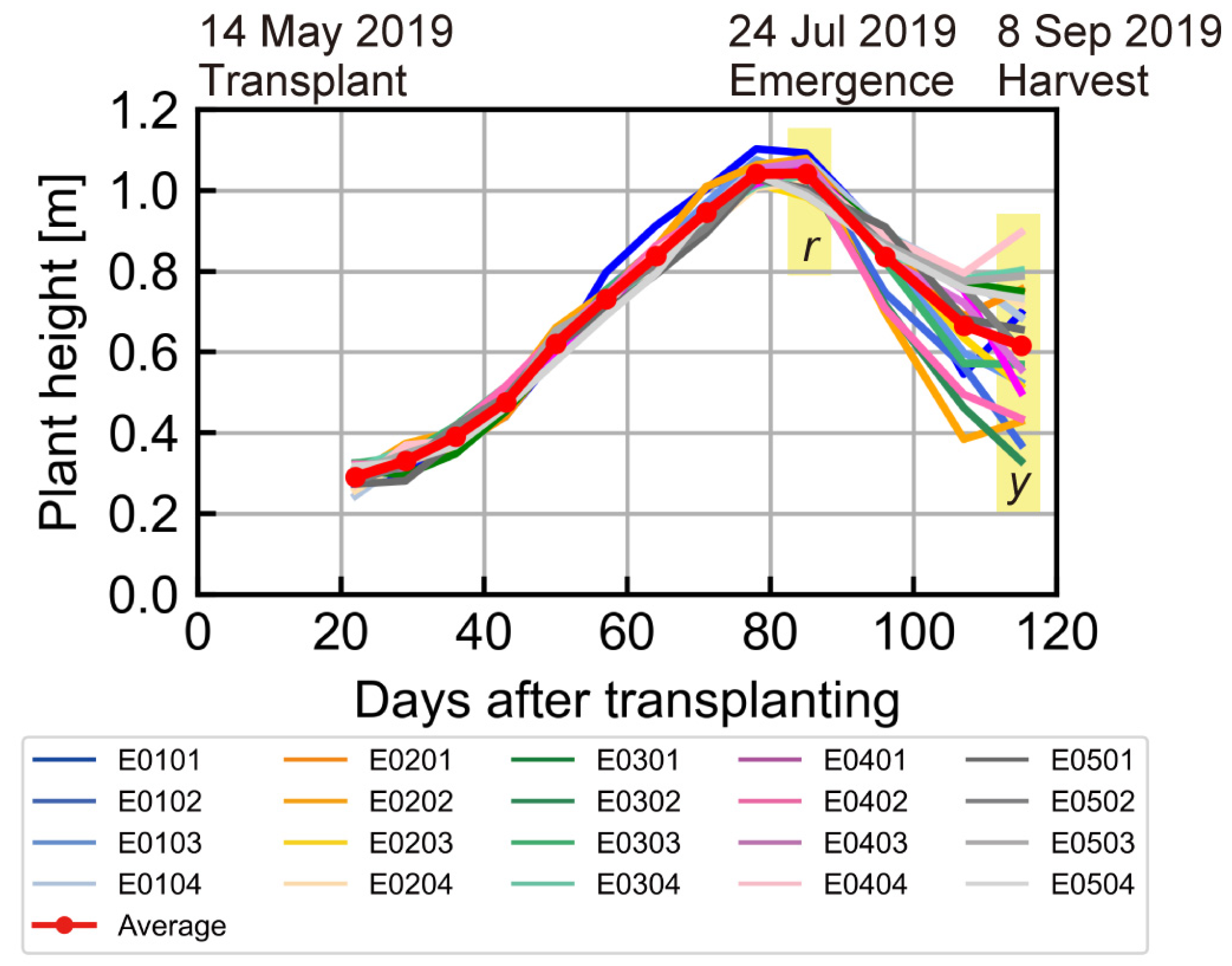
3.1. Growth of Rice Plants
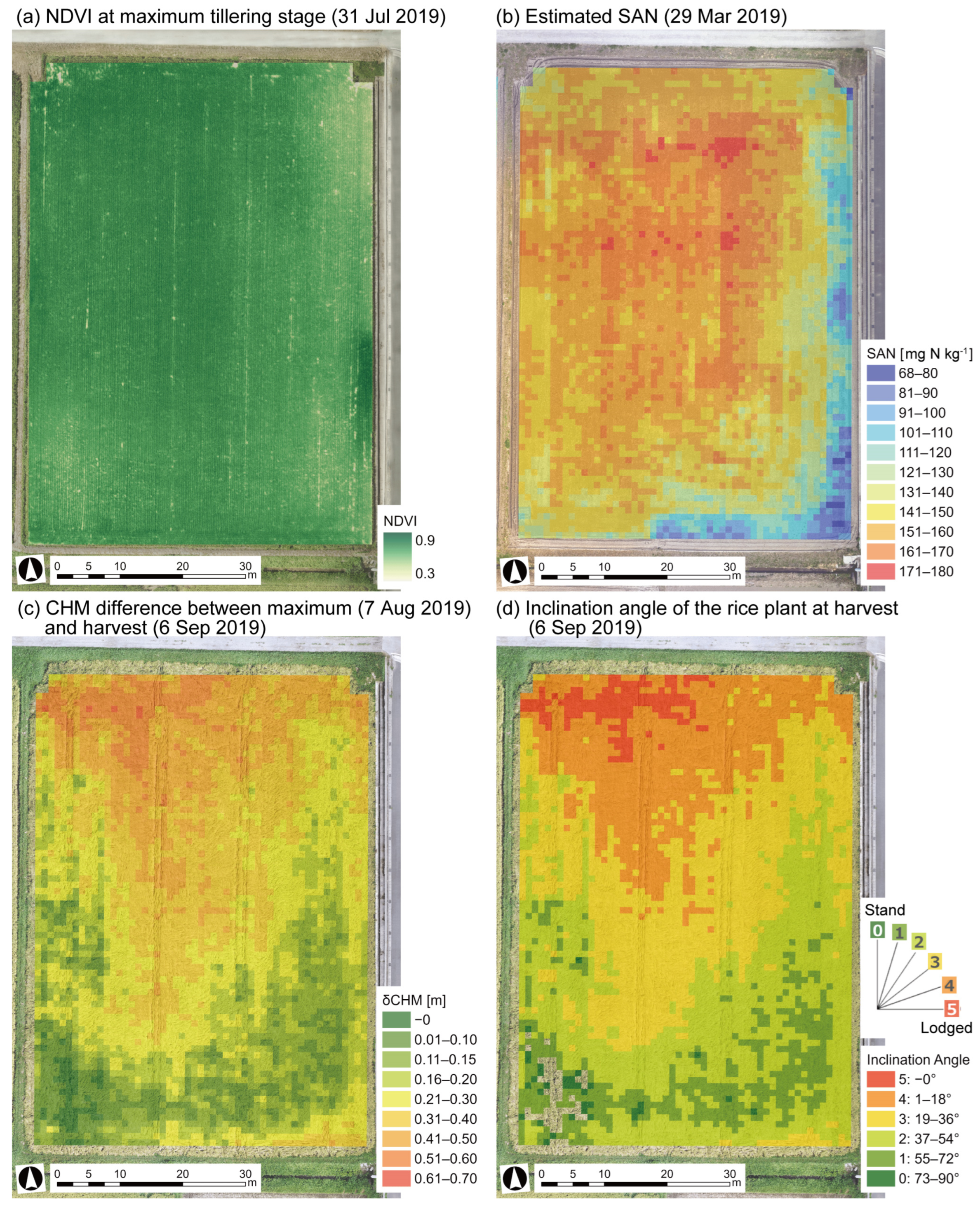
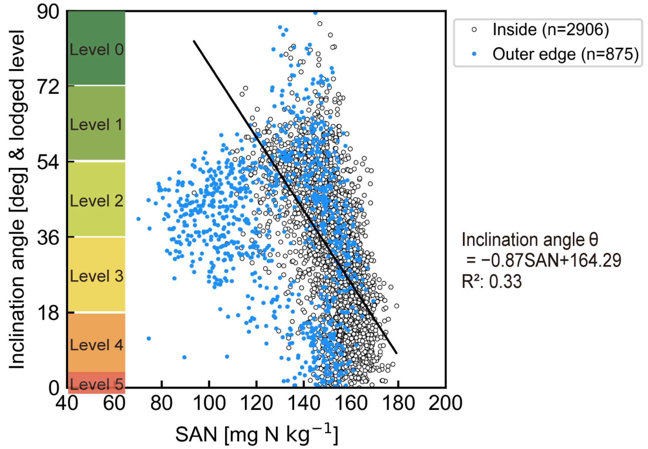
3.2. Assessment of Lodging Severity
3.3. Soil Chemical Analysis
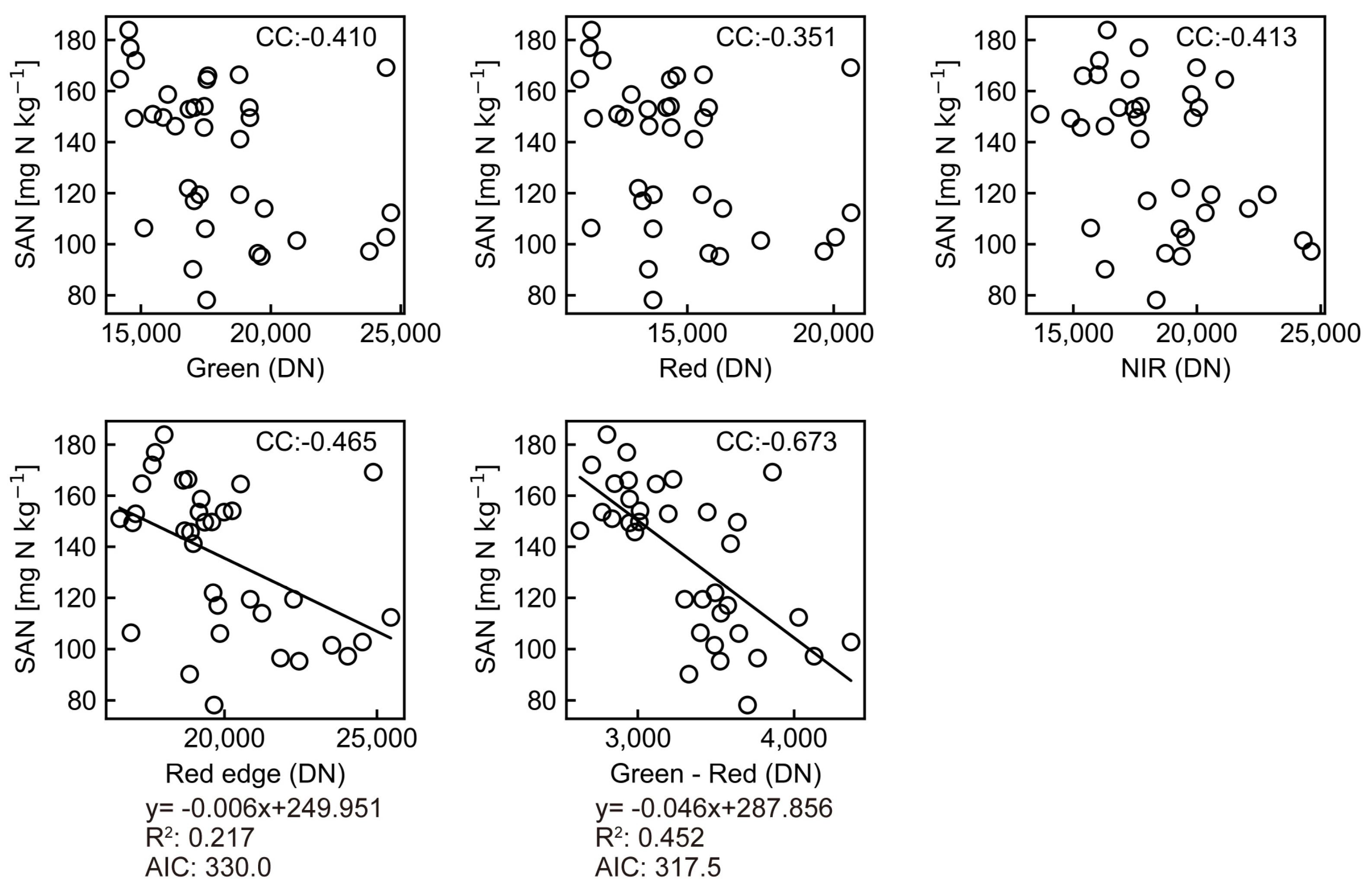
3.4. Estimate of the SAN Distribution
4. Discussion
4.1. Correlation between Rice Lodging and SAN
4.2. Factors Influencing the Accuracy of the SAN Estimating Equation
- Conduct multiple tillage during fallow periods to decompose rice residues.
- Collect soil sample and take UAS images when the soil is sufficiently dry.
- Take UAS images when the soil surface is uniform after irrigating the paddy fields [46].
- Analyze several soil surface images (described above) by machine learning [28].
5. Conclusions
Author Contributions
Funding
Institutional Review Board Statement
Informed Consent Statement
Data Availability Statement
Conflicts of Interest
References
- Kobayashi, A.; Hori, K.; Yamamoto, T.; Yano, M. Koshihikari: A Premium Short-Grain Rice Cultivar—Its Expansion and Breeding in Japan. Rice 2018, 11, 15. [Google Scholar] [CrossRef]
- Setter, T.L.; Laureles, E.V.; Mazaredo, A.M. Lodging Reduces Yield of Rice by Self-Shading and Reductions in Canopy Photosynthesis. Field Crops Res. 1997, 49, 95–106. [Google Scholar] [CrossRef]
- Iizumi, K. Current Technology and Challenges of Self-Threshing Combine Harvesters. J. Jpn. Soc. Agric. Mach. 1987, 49, 251–257. [Google Scholar] [CrossRef]
- Basak, M.N.; Sen, S.K.; Bhattacharjee, P.K. Effects of High Nitrogen Fertilization and Lodging on Rice Yield 1. Agron. J. 1962, 54, 477–480. [Google Scholar] [CrossRef]
- Zhang, W.; Wu, L.; Ding, Y.; Yao, X.; Wu, X.; Weng, F.; Li, G.; Liu, Z.; Tang, S.; Ding, C.; et al. Nitrogen Fertilizer Application Affects Lodging Resistance by Altering Secondary Cell Wall Synthesis in Japonica Rice (Oryza sativa). J. Plant Res. 2017, 130, 859–871. [Google Scholar] [CrossRef]
- Ministry of Agriculture, Forestry and Fishries (MAFF). Information for Rice Cultivation. Available online: https://www.maff.go.jp/j/seisan/gijutsuhasshin/techinfo/suitou.html (accessed on 8 February 2022).
- Dunn, B. Koshihikari Growing Guide. Available online: https://www.dpi.nsw.gov.au/__data/assets/pdf_file/0012/671979/Koshihikari-growing-guide.pdf (accessed on 20 February 2022).
- Zennoh Toyama. Optimum Fertilizer Application for Koshihikari Cultivation. Available online: http://www.ty.zennoh.or.jp/files/production_001_03.pdf (accessed on 8 February 2022).
- MAFF. Basic Guideline for Soil Fertility Enhancement. Available online: https://www.maff.go.jp/j/seisan/kankyo/hozen_type/ (accessed on 8 February 2022).
- Hyogo Prefecture. Chapter 4. Research Method of Plant Growth and Harvest. In Principle of Guidance for Rice, Wheat and Soybean; Hyogo Prefectural Government: Kobe, Japan, 2017; pp. 129–140. [Google Scholar]
- Xiang, H.; Tian, L. Development of a Low-Cost Agricultural Remote Sensing System Based on an Autonomous Unmanned Aerial Vehicle (UAV). Biosyst. Eng. 2011, 108, 174–190. [Google Scholar] [CrossRef]
- Weiss, M.; Jacob, F.; Duveiller, G. Remote Sensing for Agricultural Applications: A Meta-Review. Remote Sens. Environ. 2020, 236, 111402. [Google Scholar] [CrossRef]
- Yao, H.; Qin, R.; Chen, X. Unmanned Aerial Vehicle for Remote Sensing Applications—A Review. Remote Sens. 2019, 11, 1443. [Google Scholar] [CrossRef]
- Shahi, T.B.; Xu, C.-Y.; Neupane, A.; Guo, W. Machine Learning Methods for Precision Agriculture with UAV Imagery: A Review. Electron. Res. Arch. 2022, 30, 4277–4317. [Google Scholar] [CrossRef]
- Tao, H.; Feng, H.; Xu, L.; Miao, M.; Long, H.; Yue, J.; Li, Z.; Yang, G.; Yang, X.; Fan, L. Estimation of Crop Growth Parameters Using UAV-Based Hyperspectral Remote Sensing Data. Sensors 2020, 20, 1296. [Google Scholar] [CrossRef]
- Lu, T.; Wan, L.; Qi, S.; Gao, M. Land Cover Classification of UAV Remote Sensing Based on Transformer—CNN Hybrid Architecture. Sensors 2023, 23, 5288. [Google Scholar] [CrossRef] [PubMed]
- Mia, M.S.; Tanabe, R.; Habibi, L.N.; Hashimoto, N.; Homma, K.; Maki, M.; Matsui, T.; Tanaka, T.S.T. Multimodal Deep Learning for Rice Yield Prediction Using UAV-Based Multispectral Imagery and Weather Data. Remote Sens. 2023, 15, 2511. [Google Scholar] [CrossRef]
- Ahmadi, P.; Mansor, S.; Farjad, B.; Ghaderpour, E. Unmanned Aerial Vehicle (UAV)-Based Remote Sensing for Early-Stage Detection of Ganoderma. Remote Sens. 2022, 14, 1239. [Google Scholar] [CrossRef]
- Chauhan, S.; Darvishzadeh, R.; Boschetti, M.; Pepe, M.; Nelson, A. Remote Sensing-Based Crop Lodging Assessment: Current Status and Perspectives. ISPRS J. Photogramm. Remote Sens. 2019, 151, 124–140. [Google Scholar] [CrossRef]
- Tanaka, K.; Kondoh, A. Mapping of Rice Growth Using Low Altitude Remote Sensing by Multicopter. J. Remote Sens. Soc. Jpn. 2016, 36, 373–387. [Google Scholar] [CrossRef]
- Yang, M.-D.; Huang, K.-S.; Kuo, Y.-H.; Tsai, H.P.; Lin, L.-M.; Dempewolf, J.; Nagol, J.; Feng, M.; Atzberger, C. Spatial and Spectral Hybrid Image Classification for Rice Lodging Assessment through UAV Imagery. Remote Sens. 2017, 9, 583. [Google Scholar] [CrossRef]
- Yang, M.D.; Boubin, J.G.; Tsai, H.P.; Tseng, H.H.; Hsu, Y.C.; Stewart, C.C. Adaptive Autonomous UAV Scouting for Rice Lodging Assessment Using Edge Computing with Deep Learning EDANet. Comput. Electron. Agric. 2020, 179, 105817. [Google Scholar] [CrossRef]
- Yang, M.D.; Tseng, H.H.; Hsu, Y.C.; Tsai, H.P. Semantic Segmentation Using Deep Learning with Vegetation Indices for Rice Lodging Identification in Multi-Date UAV Visible Images. Remote Sens. 2020, 12, 633. [Google Scholar] [CrossRef]
- Mulder, V.L.; de Bruin, S.; Schaepman, M.E.; Mayr, T.R. The Use of Remote Sensing in Soil and Terrain Mapping—A Review. Geoderma 2011, 162, 1–19. [Google Scholar] [CrossRef]
- Zhang, Y.; Sui, B.; Shen, H.; Ouyang, L. Mapping Stocks of Soil Total Nitrogen Using Remote Sensing Data: A Comparison of Random Forest Models with Different Predictors. Comput. Electron. Agric. 2019, 160, 23–30. [Google Scholar] [CrossRef]
- Zhou, T.; Geng, Y.; Chen, J.; Pan, J.; Haase, D.; Lausch, A. High-Resolution Digital Mapping of Soil Organic Carbon and Soil Total Nitrogen Using DEM Derivatives, Sentinel-1 and Sentinel-2 Data Based on Machine Learning Algorithms. Sci. Total Environ. 2020, 729, 138244. [Google Scholar] [CrossRef] [PubMed]
- Zhou, T.; Geng, Y.; Ji, C.; Xu, X.; Wang, H.; Pan, J.; Bumberger, J.; Haase, D.; Lausch, A. Prediction of Soil Organic Carbon and the C:N Ratio on a National Scale Using Machine Learning and Satellite Data: A Comparison between Sentinel-2, Sentinel-3 and Landsat-8 Images. Sci. Total Environ. 2021, 755, 142661. [Google Scholar] [CrossRef] [PubMed]
- Morishita, M.; Ishitsuka, N. Estimation of Soilproperties Distribution Using UAV Observation and Machine Learning—Application of Data Augmentation to Soil Physicochemical Properties. J. Jpn. Agric. Syst. Soc. 2021, 37, 21–28. [Google Scholar] [CrossRef]
- Niwa, K.; Yokobori, J.; Hara, K.; Fueki, N.; Wakabayashi, M. Use of Remote-Sensing Data on Soil Nitrogen Availability and Wheat Growth to Estimate Factors That Affect within-Field Variation in Wheat Growth. Jpn. J. Soil Sci. Plant Nutr. 2018, 89, 544–551. [Google Scholar] [CrossRef]
- Togami, K.; Takamoto, A.; Takahashi, T. Estimating Available Nitrogen Using Total Carbon Content and Spectral Reflectance Obtained from Aerial Photography of Paddies with Continuous Organic Matter Application. Jpn. J. Soil Sci. Plant Nutr. 2022, 93, 69–76. [Google Scholar] [CrossRef]
- Japan Meteorological Agency (JMA). Historical Annual Weather Data at Tsu Station, Mie. Available online: https://www.data.jma.go.jp/obd/stats/etrn/view/annually_s.php?prec_no=53&block_no=47651&year=&month=&day=&view= (accessed on 25 April 2022).
- Jones, H.G.; Vaughan, R.A. Use of Spectral Information for Sensing Vegetation Properties and for Image Classification. In Remote Sensing of Vegetation: Principles, Techniques, and Application; Oxford University Press Inc.: New York, NY, USA, 2010; pp. 163–194. [Google Scholar]
- Lai, J.-K.; Lin, W.-S. Assessment of the Rice Panicle Initiation by Using NDVI-Based Vegetation Indexes. Appl. Sci. 2021, 11, 10076. [Google Scholar] [CrossRef]
- Iseki, K.; Matsumoto, R. Non-Destructive Shoot Biomass Evaluation Using a Handheld NDVI Sensor for Field-Grown Staking Yam (Dioscorea rotundata Poir.). Plant Prod. Sci. 2019, 22, 301–310. [Google Scholar] [CrossRef]
- Uchiyama, S. Analysis by RTKLIB. In Proceedings of the Open Educational Material for Acquiring High-Definition Topographic Information, Sapporo, Japan, 29 July 2018. [Google Scholar]
- Takasu, T. RTKLIB ver. 2.4.2 Manual. Available online: http://www.rtklib.com/rtklib.htm (accessed on 21 April 2019).
- Geospatial Information Authority of Japan (GSI). GEONET. Available online: https://www.gsi.go.jp/ENGLISH/geonet_english.html (accessed on 5 August 2019).
- Hokkaido Research Organization (HRO). Continuous Measurement of pH(Water) and EC. In Anlysis Method for Soil and Crop Nutrient 2012; HRO Agricultural Research Department: Sapporo, Japan, 2012; pp. 59–62. [Google Scholar]
- National Agriculture and Food Research Organization (NARO). A Manual for Simple and Rapid Assessment of Available Nitrogen in Paddy Soil. Available online: http://www.naro.affrc.go.jp/publicity_report/publication/pamphlet/tech-pamph/062019.html (accessed on 5 March 2019).
- Hama, A.; Kondho, A.; Tanaka, K.; Den, H. Comparison and Consideration of Near-Infrared Cameras for Drones: RedEdge and Yubaflex. J. Remote Sens. Soc. Jpn. 2018, 38, 451–457. [Google Scholar] [CrossRef]
- Micasense. Best practices: Collecting Data with MicaSense Sensors. Available online: https://support.micasense.com/hc/en-us (accessed on 6 March 2022).
- Zhang, D.; Zhou, G. Estimation of Soil Moisture from Optical and Thermal Remote Sensing: A Review. Sensors 2016, 16, 1308. [Google Scholar] [CrossRef]
- Wang, X.; Zhang, F.; Ding, J.; Kung, H.; Latif, A.; Johnson, V.C. Estimation of Soil Salt Content (SSC) in the Ebinur Lake Wetland National Nature Reserve (ELWNNR), Northwest China, Based on a Bootstrap-BP Neural Network Model and Optimal Spectral Indices. Sci. Total Environ. 2018, 615, 918–930. [Google Scholar] [CrossRef]
- Wilke, N.; Siegmann, B.; Klingbeil, L.; Burkart, A.; Kraska, T.; Muller, O.; van Doorn, A.; Heinemann, S.; Rascher, U. Quantifying Lodging Percentage and Lodging Severity Using a UAV-Based Canopy Height Model Combined with an Objective Threshold Approach. Remote Sens. 2019, 11, 515. [Google Scholar] [CrossRef]
- Djeddaoui, F.; Chadli, M.; Gloaguen, R. Desertification Susceptibility Mapping Using Logistic Regression Analysis in the Djelfa Area, Algeria. Remote Sens. 2017, 9, 1031. [Google Scholar] [CrossRef]
- Shiga, H.; Fukuhara, M.; Ogawa, S. Mapping Soil Organic Matter of Submerged Paddy Using Landsat TM Data. Jpn. J. Soil Sci. Plant Nutr. 1989, 60, 432–436. [Google Scholar] [CrossRef]


| Soil Indicators | Field A | Field B | All | |
|---|---|---|---|---|
| Depth of Plow Layer [mm] | Mean | 104.3 | 140 | 119.6 |
| SD | 11.27 | 19.55 | 23.46 | |
| CV | 10.8 | 14.0 | 19.6 | |
| Water Content [%] | Mean | 31.6 | 30.5 | 31.1 |
| SD | 1.27 | 2.45 | 1.92 | |
| CV | 4.0 | 8.0 | 6.2 | |
| pH | Mean | 5.67 | 6.21 | 5.90 |
| SD | 0.187 | 0.157 | 0.320 | |
| CV | 3.3 | 2.5 | 5.4 | |
| EC [dS m−1] | Mean | 0.07 | 0.10 | 0.08 |
| SD | 0.025 | 0.025 | 0.028 | |
| CV | 33.8 | 24.9 | 32.8 | |
| SAN [mg N kg−1] | Mean | 156.0 | 108.5 | 135.6 |
| SD | 14.10 | 20.54 | 29.21 | |
| CV | 9.0 | 18.9 | 21.5 | |
| Total Nitrogen [%] | Mean | 0.17 | 0.16 | 0.17 |
| SD | 0.012 | 0.015 | 0.011 | |
| CV | 7.3 | 9.2 | 8.3 | |
| Total Carbon [%] | Mean | 1.99 | 2.12 | 2.04 |
| SD | 0.158 | 0.255 | 0.212 | |
| CV | 8.0 | 12.0 | 10.4 | |
| C/N | Mean | 11.5 | 12.9 | 12.1 |
| SD | 0.66 | 0.80 | 0.97 | |
| CV | 5.7 | 6.3 | 8.0 | |
| Explanatory Variables | Explained Variables | |||
|---|---|---|---|---|
| TN | TC | SAN | ||
| Single Band | Gr | −0.094 | 0.179 | −0.410 |
| Red | −0.055 | 0.191 | −0.351 | |
| RE | −0.093 | 0.216 | −0.465 | |
| NIR | −0.260 | −0.184 | −0.413 | |
| Spectral Index | Gr − Red | −0.300 | 0.071 | −0.673 |
| Gr − RE | −0.038 | −0.004 | −0.050 | |
| Gr − NIR | 0.167 | 0.403 | −0.039 | |
| Red − RE | 0.077 | −0.033 | 0.212 | |
| Red − NIR | 0.232 | 0.413 | 0.083 | |
| RE − NIR | 0.260 | 0.566 | −0.020 | |
| Gr + Red | −0.076 | 0.185 | −0.383 | |
| Gr + RE | −0.095 | 0.200 | −0.446 | |
| Gr + NIR | −0.193 | 0.007 | −0.460 | |
| Red + RE | −0.075 | 0.208 | −0.417 | |
| Red + NIR | −0.179 | 0.000 | −0.430 | |
| RE + NIR | −0.192 | 0.008 | −0.468 | |
| Gr/Red | −0.261 | −0.156 | −0.265 | |
| Gr/RE | −0.055 | 0.012 | −0.134 | |
| Gr/NIR | 0.154 | 0.379 | −0.050 | |
| Red/RE | 0.019 | 0.056 | −0.051 | |
| Red/NIR | 0.183 | 0.383 | −0.006 | |
| RE/NIR | 0.256 | 0.533 | 0.022 | |
| NDI | Gr, Red | −0.261 | −0.159 | −0.263 |
| Gr, RE | −0.063 | 0.015 | −0.148 | |
| Gr, NIR | 0.147 | 0.376 | −0.065 | |
| Red, RE | 0.012 | 0.054 | −0.062 | |
| Red, NIR | 0.177 | 0.377 | −0.020 | |
| RE, NIR | 0.264 | 0.535 | 0.023 | |
Disclaimer/Publisher’s Note: The statements, opinions and data contained in all publications are solely those of the individual author(s) and contributor(s) and not of MDPI and/or the editor(s). MDPI and/or the editor(s) disclaim responsibility for any injury to people or property resulting from any ideas, methods, instructions or products referred to in the content. |
© 2023 by the authors. Licensee MDPI, Basel, Switzerland. This article is an open access article distributed under the terms and conditions of the Creative Commons Attribution (CC BY) license (https://creativecommons.org/licenses/by/4.0/).
Share and Cite
Sato, N.K.; Tsuji, T.; Iijima, Y.; Sekiya, N.; Watanabe, K. Predicting Rice Lodging Risk from the Distribution of Available Nitrogen in Soil Using UAS Images in a Paddy Field. Sensors 2023, 23, 6466. https://doi.org/10.3390/s23146466
Sato NK, Tsuji T, Iijima Y, Sekiya N, Watanabe K. Predicting Rice Lodging Risk from the Distribution of Available Nitrogen in Soil Using UAS Images in a Paddy Field. Sensors. 2023; 23(14):6466. https://doi.org/10.3390/s23146466
Chicago/Turabian StyleSato, Nozomi Kaneko, Takeshi Tsuji, Yoshihiro Iijima, Nobuhito Sekiya, and Kunio Watanabe. 2023. "Predicting Rice Lodging Risk from the Distribution of Available Nitrogen in Soil Using UAS Images in a Paddy Field" Sensors 23, no. 14: 6466. https://doi.org/10.3390/s23146466
APA StyleSato, N. K., Tsuji, T., Iijima, Y., Sekiya, N., & Watanabe, K. (2023). Predicting Rice Lodging Risk from the Distribution of Available Nitrogen in Soil Using UAS Images in a Paddy Field. Sensors, 23(14), 6466. https://doi.org/10.3390/s23146466