1. Introduction
Neural networks are well known to achieve comparable or superior performance to humans in many challenging tasks, including image classification [
1], speech recognition [
2] and game playing [
3]. However, a growing body of research demonstrates that neural networks also face various security threats, which include evasion [
4], poisoning [
5], extraction [
6], and inference [
7]. The threat of evasion attacks against machine learning models was first investigated by [
8]. Subsequently, Szegedy et al. [
9] experimentally discovered the existence of adversarial examples, which can be effectively used in evasion attacks against neural networks. Since then, adversarial examples, as an “intriguing property” of neural networks [
9], have attracted increasing research attention.
Adversarial examples were originally synthesized by adding carefully crafted perturbations to benign examples. These perturbations are imperceptible to humans but can easily fool a neural network model. Subsequently, other types of adversarial examples have been presented, such as natural adversarial examples [
10], semantic adversarial examples [
11], and unrestricted adversarial examples [
12]. The concept of adversarial examples has accordingly been generalized to refer to a category of examples that can fool neural networks but not humans.
In this paper, we present another intriguing property of neural networks: the fact that well-trained models believe some examples to be recognizable objects (often with high confidence), while humans cannot recognize such examples. We refer to this category of examples, namely those that can be recognized by neural networks but cannot be recognized by humans, as “fooling examples”. As is evident, the fooling example is a new concept that differs from the adversarial example, as the latter refers to an example that can be recognized by both humans and neural networks, although neural networks give an incorrect prediction.
Figure 1 shows the prediction results of a natural example and a fooling example, along with their corresponding attention maps [
13,
14] on ResNet-50 [
1]. We can see that just like the natural example, the fooling example is also recognized as “meerkat” by the network, with even higher confidence.
The contributions of this work can be summarized as follows:
We propose the concept of “fooling examples” and discuss the ways in which they differ from adversarial examples.
We propose an iterative method for generating fooling examples, which combines techniques such as momentum, diverse inputs, and translation invariance to improve the transferability of fooling examples.
We systematically evaluate the performance of our proposed method. The results indicate that fooling examples can not only be generated on white-box models, but can also be transferred to black-box models and even recognized by real-world computer vision systems.
2. Related Work
To the best of our knowledge, the concept of “fooling examples” is proposed for the first time in this paper; as a result, there is little existing related work in this field. Perhaps the most relevant work is the study conducted by Nguyen et al. in [
15]. The authors found that deep neural networks can be easily fooled into making high-confidence predictions for unrecognizable images, which are referred to as “fooling images”. In [
15], the authors mainly used two evolutionary algorithms [
16] and one gradient ascent algorithm [
17] to find unrecognizable examples. The gradient ascent algorithm is derived from [
17], and it maximizes the softmax output for classes using gradient ascent in the image space. However, the method we proposed for generating fooling examples is an upgraded version of the iterative fast gradient sign method (I-FGSM) [
18]. It combines techniques such as momentum [
19], diverse inputs [
20], and translation invariance [
21], and can effectively improve the transferability of fooling examples.
Since our method of generating fooling examples is inspired by existing methods of generating adversarial examples [
22,
23,
24], we also introduce some related work on adversarial examples here. Szegedy et al. [
9] were the first to propose the concept of adversarial examples, and accordingly developed a box-constrained L-BFGS method for generating such examples. Goodfellow et al. proposed the fast gradient sign method (FGSM) [
25] for efficiently generating adversarial examples. Kurakin et al. extended FGSM to an iterative version, i.e., I-FGSM [
18]. To improve the transferability of adversarial examples, Dong et al. proposed the momentum iterative fast gradient sign method (MI-FGSM) [
19]; for their part, Xie et al. proposed the diverse inputs iterative fast gradient sign method (DI
2-FGSM) [
20], after which Dong et al. proposed the translation-invariant iterative fast gradient sign method (TI
2-FGSM) [
21].
3. Fooling Examples vs. Adversarial Examples
We believe that the fooling examples we present in this paper are fundamentally different from the adversarial examples that have been extensively studied. In this section, we provide a formal characterization of adversarial examples and fooling examples.
Let be the set of all input examples under consideration. We consider a neural network classifier that can give a prediction for any example in , where denotes the set of categories of natural examples that can be recognized by the classifier. Suppose is an oracle that takes an example in and outputs one of labels, or a label if the example is unrecognizable. In addition, we denote the discriminator of humans as ; that is, the humans can recognize an example in as a label in or will assign a label if the example is unrecognizable. We assume . Equipped with these notations, we provide the following definitions for adversarial examples and fooling examples.
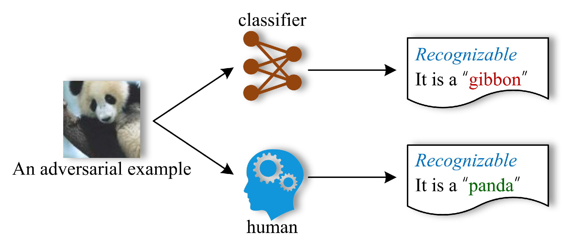
Definition 1 (Adversarial examples). An adversarial example is defined to be any example in .
In other words, the adversarial example can be recognized by both humans and the classifier; however, the classifier gives an incorrect prediction.
Figure 2 illustrates the recognization results of an adversarial example by the classifier and the human.
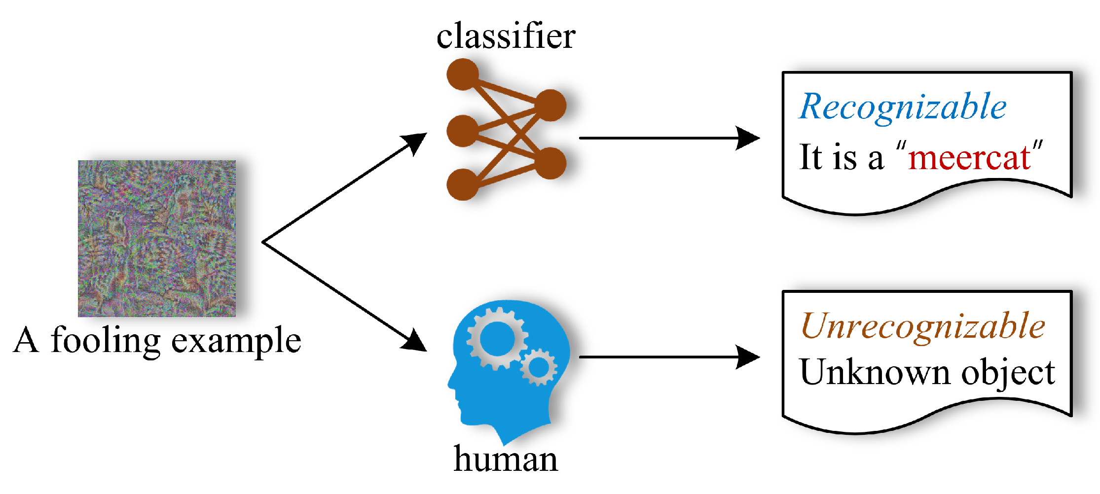
Definition 2 (Fooling examples). A fooling example is defined to be any example in .
In other words, the fooling example cannot be recognized by humans; however, the classifier believes it to be a recognizable object (even with high confidence).
Figure 3 illustrates the recognization results of a fooling example by the classifier and the human.
4. Methodology
Fooling examples are defined as examples that can be recognized by neural networks, but cannot be recognized by humans. Theoretically, the generation of fooling examples requires human intervention, which may be a process of human–machine cooperation. However, human involvement will further complicate the process of generating fooling examples. In fact, the generation of fooling examples can be accomplished in a relatively simple way, which is described in detail in this section.
4.1. Problem Specification
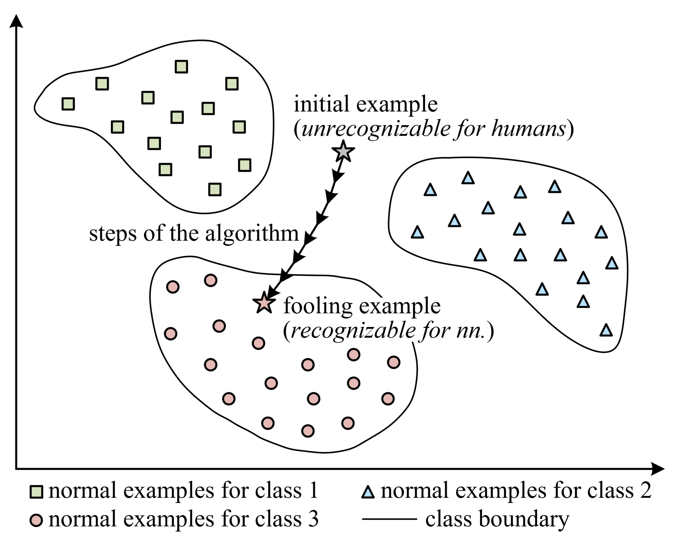
As illustrated in
Figure 4, the process of generating a fooling example can be divided into two phases: (a) finding an initial example that is unrecognizable for humans (e.g., random noise, all-white or all-black images); (b) making minor changes to the initial example using a specific algorithm and obtaining a fooling example that is recognizable for neural networks. Because the fooling example has a very small distinction from the initial example, it is unrecognizable for humans, but is recognizable for neural networks.
Next, we present a formalized description of the process of fooling example generation. Let
denote the initial example and
denote the generated fooling example. Given a classifier
f, we want the fooling example
to be recognized as a label
y, i.e.,
. If the adversary’s loss function of the classifier is denoted as
J, the process of generating the fooling example
can be formally expressed as a matter of solving the following constrained optimization problem:
where
is the maximum threshold of the
-norm distance (i.e.,
) between
and
, and guarantees that
has a very small distinction from
; thus,
is still unrecognizable for humans.
Solving the optimization problem (
1) requires calculating the gradient of the loss function with respect to the input. Since the problem (
1) is similar to the problem of generating targeted adversarial examples, the classical methods for generating adversarial examples, such as I-FGSM [
18], MI-FGSM [
19], DI
2-FGSM [
20], and TI
2-FGSM [
21], can be extended for generating fooling examples.
4.2. Gradient-Based Iterative Methods
In this paper, we consider four basic gradient-based iterative methods for generating fooling examples.
Iterative Fast Gradient Sign Method for Generating Fooling Examples (I-FGSMfool). I-FGSM [
18] can be extended into a method for generating fooling examples, which is denoted as I-FGSM
fool and can be expressed as follows:
where
means that
is initialized with an example that is unrecognizable for humans (e.g., random-noise, all-white or all-black images);
denotes the intermediate example at the
t-th iteration;
indicates that the example generated in each iteration is clipped within the
-ball of the initial example
; finally,
is the step size at each iteration.
Momentum Iterative Fast Gradient Sign Method for Generating Fooling Examples (MI-FGSMfool). Similarly, MI-FGSM [
19] can be extended into a method for generating fooling examples, which is termed as MI-FGSM
fool and can be expressed as follows:
where
is the decay factor of the momentum term, while
is the accumulated gradient at the
t-th iteration.
Diverse Inputs Iterative Fast Gradient Sign Method for Generating Fooling Examples (DI2-FGSMfool). DI
2-FGSM [
20] is developed for generating transferable adversarial examples by creating diverse input patterns. DI
2-FGSM can also be extended into a method for generating transferable fooling examples, which is referred to as DI
2-FGSM
fool and can be expressed as follows:
where
indicates a random transformation on the input
with a probability
p. This transformation may take the form of, e.g., random resizing and padding.
Translation-Invariant Iterative Fast Gradient Sign Method for Generating Fooling Examples (TI2-FGSMfool). Done et al. [
21] proposed a translation-invariant method, named TI
2-FGSM, to generate more transferable adversarial examples against the defense models. TI
2-FGSM can also be extended into a method for generating transferable fooling examples, which is termed as TI
2-FGSM
fool and can be expressed as follows:
where
denotes a predefined kernel, which can be uniform, linear, or Gaussian.
4.3. Generating Algorithm
The above I-FGSM
fool, MI-FGSM
fool, DI
2-FGSM
fool, and TI
2-FGSM
fool can be integrated together to form a powerful method, which is referred to as MTI-DI
2-FGSM
fool and presented in Algorithm 1. MTI-DI
2-FGSM
fool is built on the basis of I-FGSM
fool by taking advantage of the momentum, diverse inputs, and translation invariance. On the one hand, MTI-DI
2-FGSM
fool is able to achieve high success rates under white-box scenarios; on the other hand, MTI-DI
2-FGSM
fool can effectively improve the transferability of fooling examples under black-box scenarios.
| Algorithm 1 MTI-DI2-FGSMfool for generating fooling examples. |
Input: A classifier f; a class label y; adversary’s loss function J; number of iterations T; step size ; perturbation threshold ; decay factor ; transformation probability p and predefined kernel . Output: A fooling example with label y. - 1:
Set . ⊳ random-noise, all-white or all-black. - 2:
Let , . - 3:
for do - 4:
Transform and get ; ⊳ Apply DI - 5:
Input to f and calculate the gradient: ; - 6:
; ⊳ Apply TI - 7:
; ⊳ Apply MI - 8:
; ⊳ Apply FGSM - 9:
end for - 10:
return .
|
5. Experiments
5.1. Experimental Setup
Dataset. Our goal is to generate fooling examples that can be recognized by neural networks. These fooling examples are crafted based on the initial examples by using the algorithm MTI-DI
2-FGSM
fool. In our experiments, we consider four types of initial examples: random Gaussian noise images, random uniform noise images, all-white images, and all-black images. Additionally, we need to set the labels that neural networks will recognize the fooling examples as. These labels are taken from an ImageNet-compatible dataset at
https://www.kaggle.com/competitions/nips-2017-targeted-adversarial-attack/data (accessed on 16 March 2023), which contains 1000 target labels.
Models. We consider four pretrained ImageNet models: ResNet-50 (Res50) [
1], Inception-v3 (Inc-v3) [
26], DenseNet-121 (Dense121) [
27], and VGG16 [
28]. These models have diverse architectures and are all publicly available at
https://keras.io/api/applications/ (accessed on 16 March 2023).
Parameter settings and the method for comparison. Following the settings outlined in [
29], for MTI-DI
2-FGSM
fool, the number of iterations
T is set to be 300 and the step size
is set to be 2; the decay factor
is set to be 1.0; the transformation probability
p is set to be 0.7; finally, the kernel
is set to be a Gaussian kernel with size of 5. To provide an objective evaluation of our proposed MTI-DI
2-FGSM
fool, we compare it with the gradient ascent method [
15].
White-box and black-box scenarios. In the white-box scenario, we have full access to the model’s architecture and parameters, thus we can use this information to generate fooling examples by directly calculating the gradient of the loss function with respect to the input. In the black-box scenario, we have no direct access to the target model’s architecture or parameters. We may only have access to the model’s input and output. In this case, we can generate fooling examples on one or multiple source models, and then directly feed them to the target model. By leveraging the transferability of fooling examples, the target model may recognize them as the specified objects.
5.2. Effect of Loss Function
As for generating adversarial examples, Cross-Entropy (CE) [
30] is the most commonly adopted loss function for many attacks. To improve the transferability of the generated adversarial examples, several different loss functions have been developed, such as Po+Trip [
31] and logit [
29]. We also tested the effect of different loss functions (CE, Po+Trip, and logit) on the success rate of fooling example generation. In more detail, the initial examples are all set to random Gaussian noise images. The maximum threshold
is set to 32. Res50 is used as the source model for fooling example generation. The generated fooling examples are then input into different models and the success rates are observed. The results are presented in
Figure 5. As the results show, in the white-box scenario (i.e., on Res50), all three loss functions perform well in generating fooling examples, with success rates close to 100%. However, in the black-box scenario (i.e., on Inc-v3, Dense121, and VGG16), the Logit loss outperforms CE and To+Trip. It is therefore clear that use of the Logit loss produces higher-quality fooling examples; accordingly, Logit loss is used as the default loss function in the following experiments.
5.3. Effect of Threshold
In the generation of perturbation-based adversarial examples, the parameter
serves as the maximum threshold for restricting the distance between adversarial examples and original benign examples. In our fooling example generation methods, the parameter
is used to restrict the distance between the generated fooling examples and the original initial examples, which guarantees that, like the initial examples, the fooling examples cannot be recognized by humans. We tested the effect of threshold
on the success rate of fooling examples. The results are shown in
Figure 6. As we can observe, in the white-box scenario (i.e., on Res50), the value of
has little effect on the success rate of fooling examples, which remains consistently close to 100%. In the black-box scenario (i.e., on Inc-v3, Dense121 and VGG16), the success rates tend to decrease when
. We accordingly conclude that the optimal value of
is 32; as such, the parameter
takes the value of 32 by default in the following experiments.
5.4. Taking a Look at Fooling Examples
We will now take a look at the fooling examples.
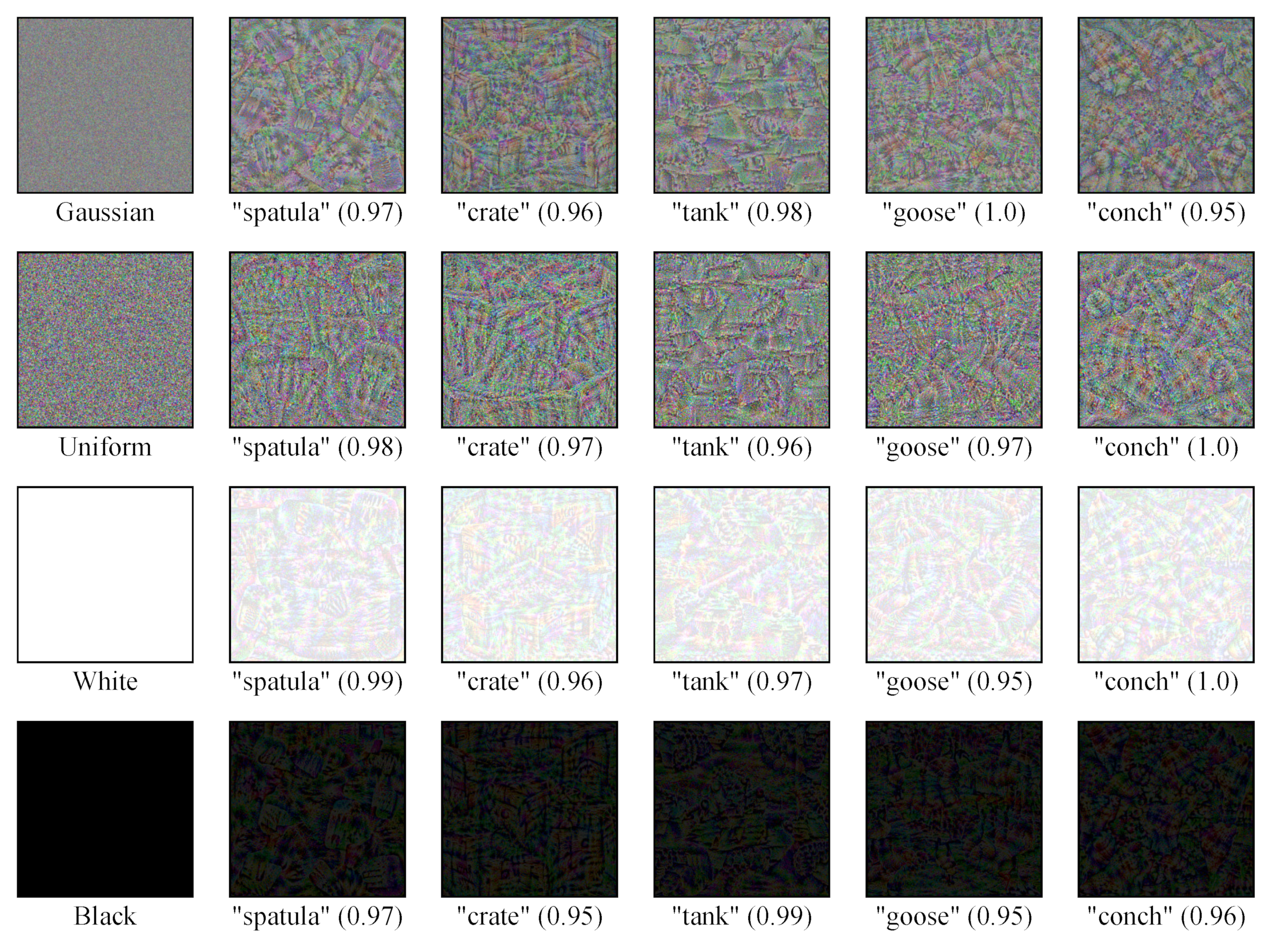
Figure 7 visualizes some randomly selected fooling examples generated from different initial examples. As we can observe, all these fooling examples are recognized as natural objects by Res50 with very high confidence. However, we humans are completely unable to recognize these fooling examples.
5.5. Generating on a Single Model
We next opt to conduct more extensive experiments. First, we fully test the generation of fooling examples on a single model. Specifically, one model (selected from Res50, Inc-v3, Dense121, and VGG16) is used as the source model to generate fooling examples, after which these generated fooling examples are then tested on all models. The success rates are shown in
Table 1; here, the rows represent the source models, and the columns represent the target models. When the source model and target model are the same, it indicates a white-box scenario, in which the generation of fooling examples utilizes the source model’s architecture and parameters; when the source model and target model are different, it indicates a black-box scenario, in which the fooling examples generated on the source model are transferred (i.e., directly input) to the target model. From
Table 1, we can observe the following: (a) In the white-box scenario, compared to the gradient ascent method [
15], our proposed method has a slightly lower success rate in generating fooling examples in some cases. However, the overall success rate of generating fooling examples in the white-box scenario remains very high, nearly reaching 100%, and is almost unaffected by the settings of initial examples; (b) In the black-box scenario, compared to the gradient ascent method [
15], our method achieves a significantly higher success rate in generating fooling examples that are recognized by the target model as the specific objects. We can also observe that the transfer rate of fooling examples is related to the settings of initial examples. Notably, the transfer rate of fooling examples generated from the random Gaussian noise and all-black images is significantly higher than that of fooling examples generated from the random uniform noise and all-white images; (c) The fooling examples generated on Inc-v3 are difficult to transfer to other models (i.e., Res50, Dense121 and VGG16), while the fooling examples generated on other models are also difficult to transfer to Inc-v3.
5.6. Generating on an Ensemble of Models
In this section, we test the generation of fooling examples on an ensemble of models. In these experiments, we opt to integrate any three of the four models (i.e., Res50, Inc-v3, Dense121, and VGG16) in order to create an ensemble model for generating fooling examples in the white-box scenario, while the remaining (hold-out) model is used as the black-box model to test the fooling examples. We follow the ensemble strategy proposed in [
19] to generate fooling examples on multiple models simultaneously. The success rates are presented in
Table 2. From the table, we can observe that compared to the gradient ascent method [
15], our method has a slight decrease in the success rate of generating fooling examples on an ensemble model in the white-box scenario. However, in the black-box scenario, our method demonstrates a significant improvement in transferability of fooling examples. We can also observe that compared to the fooling examples generated on a single model, those generated on an ensemble model are significantly more transferable. For MTI-DI
2-FGSM
fool, the transfer rate of fooling examples generated from all-black images is the highest, with an average of 64.8%. Contrarily, the transfer rate of fooling examples generated from the random uniform noise images is the lowest, with an average of 8.2%. We can accordingly conclude that the transfer rate of fooling examples is closely related to both the form of source models and the settings of initial examples.
5.7. Fooling Google Cloud Vision API
We further test the fooling examples on a real-world computer vision system—Google Cloud Vison API [
32]. The Google Cloud Vision API encapsulates powerful machine learning models in an easy-to-use API and is able to quickly classify images into thousands of categories (e.g., “tower”, “lion”, and “sailboat”). We generate fooling examples on an ensemble of four diverse models (i.e., Res50, Inc-v3, Dense121 and VGG 16). The generating algorithm is MTI-DI
2-FGSM
fool. The maximum perturbation threshold
is set to 32 and the number of iterations
T is set to 300. The loss function
J takes the form of logit loss. The generated fooling examples are sent to the API to observe whether the API classifies the fooling exmaples as the target labels. It is worth noting that for an input image, the API returns up to 10 labels (with confidence
), and the labels returned by the API are not exactly the same as the labels of the ImageNet models. Therefore, as long as the labels returned by the API contain one label that is semantically similar to the target label, we consider the fooling example to be successfully recognized by the API.
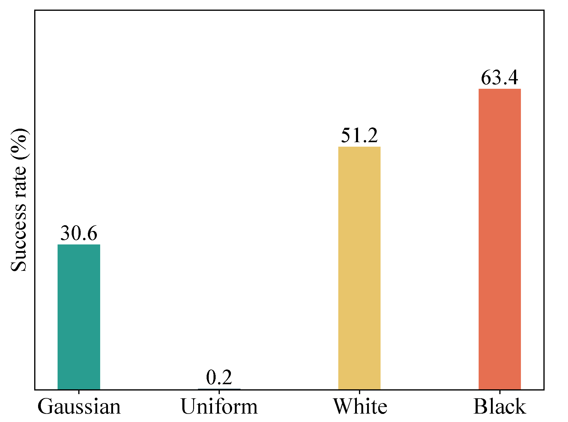
Figure 8 reports the success rates of recognition of fooling examples by the API. As we can observe, the success rate of fooling examples generated from all-black initial images is the highest (63.4%), followed by fooling examples generated from all-white initial images, with a success rate of 51.2%. The success rate of fooling examples generated from random uniform noise images is the lowest, at only 0.2%.
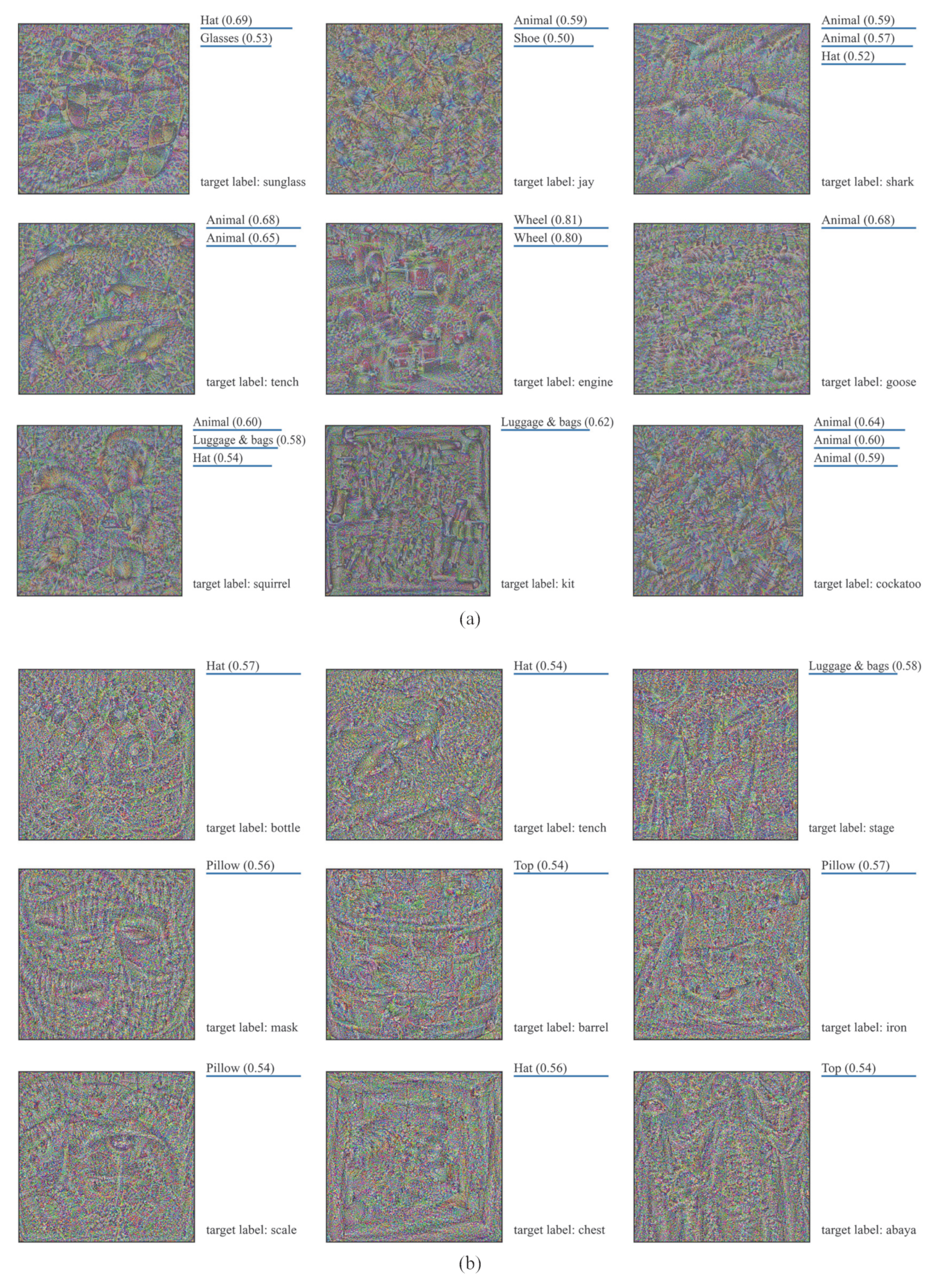
Figure 9 shows some fooling examples generated from random Gaussian or uniform noise images, as well as the API recognition results. It can be seen that the fooling examples generated from random Gaussian noise images are usually recognized by the API as categories that are semantically similar to the target labels, for example, a fooling example with the target label “shark” was recognized as an “animal” by the API. For the fooling examples generated from random uniform noise images, the API hardly recognizes them as target labels.
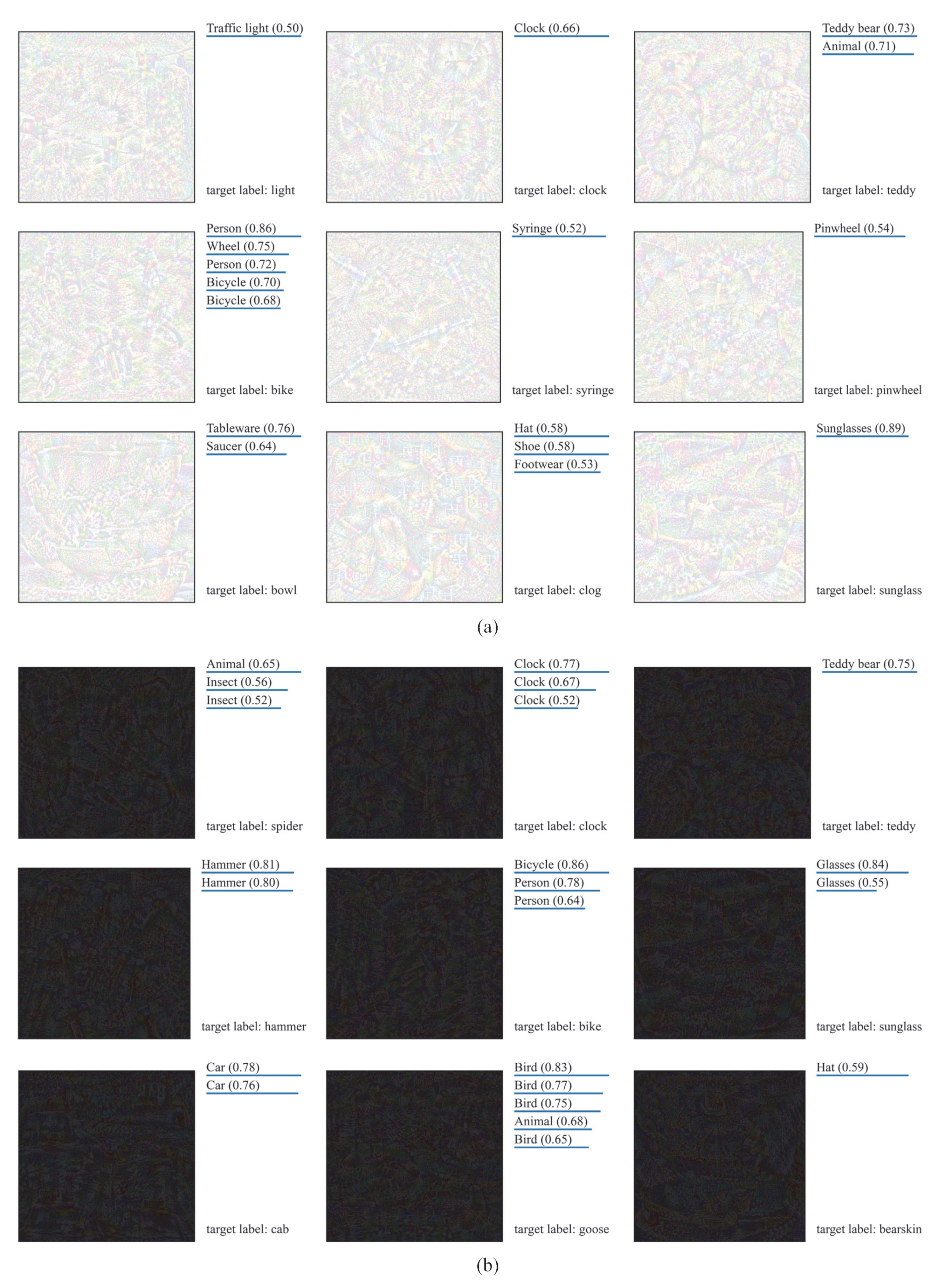
Figure 10 shows some fooling examples generated from all-white or all-black initial images, as well as the API recognition results. It can be seen that the success rate of the API correctly recognizing these fooling examples is quite high, and these fooling examples can make the API accurately recognize them as the target labels. For example, a fooling examples generated from an all-white initial image with the target label “teddy” was recognized by the API as “Teddy bear” with a confidence of 0.73; a fooling example generated from an all-black initial image with the target label “hammer” was recognized by the API as “Hammer” with a confidence of 0.81.
6. Conclusions
In this paper, we propose the concept of fooling examples, which refer to examples that can be recognized by neural networks but not by humans. We first discuss the differences between fooling and adversarial examples. Next, we develop an iterative method for generating fooling examples, which combines techniques such as momentum, diverse inputs, and translation invariance to improve the transferability of fooling examples. Finally, we conduct extensive experiments on well-trained ImageNet models to generate fooling examples. The results show that fooling examples can not only be easily generated in the white-box scenario, but also exhibit strong transferability across different models in the black-box scenario.
Author Contributions
Conceptualization, M.Z. and C.Q.; methodology, M.Z.; software, Y.C.; validation, M.Z., Y.C. and C.Q.; formal analysis, C.Q.; investigation, Y.C.; resources, M.Z.; data curation, Y.C.; writing—original draft preparation, M.Z.; writing—review and editing, C.Q.; visualization, Y.C.; supervision, M.Z.; project administration, M.Z.; funding acquisition, M.Z. All authors have read and agreed to the published version of the manuscript.
Funding
This research was funded by the Foundation of National Key Laboratory of Science and Technology on Information System Security (No. 6142111).
Institutional Review Board Statement
Not applicable.
Informed Consent Statement
Not applicable.
Data Availability Statement
Conflicts of Interest
The authors declare no conflict of interest.
References
- He, K.; Zhang, X.; Ren, S.; Sun, J. Deep Residual Learning for Image Recognition. In Proceedings of the 2016 IEEE Conference on Computer Vision and Pattern Recognition, Las Vegas, NV, USA, 26 June–1 July 2016; pp. 770–778. [Google Scholar]
- Graves, A.; Mohamed, A.; Hinton, G.E. Speech Recognition with Deep Recurrent Neural Networks. In Proceedings of the 2013 IEEE International Conference on Acoustics, Speech and Signal Processing, Vancouver, BC, Canada, 26–31 May 2013; pp. 6645–6649. [Google Scholar]
- Tomlin, N.; He, A.; Klein, D. Understanding Game-Playing Agents with Natural Language Annotations. In Proceedings of the 60th Annual Meeting of the Association for Computational Linguistics, Dublin, Ireland, 22–27 May 2022; pp. 797–807. [Google Scholar]
- Zhang, J.; Li, B.; Xu, J.; Wu, S.; Ding, S.; Zhang, L.; Wu, C. Towards efficient data free black-box adversarial attack. In Proceedings of the IEEE/CVF Conference on Computer Vision and Pattern Recognition, New Orleans, LA, USA, 19–24 June 2022; pp. 15115–15125. [Google Scholar]
- Huang, W.R.; Geiping, J.; Fowl, L.; Taylor, G.; Goldstein, T. Metapoison: Practical general-purpose clean-label data poisoning. Adv. Neural Inf. Process. Syst. 2020, 33, 12080–12091. [Google Scholar]
- Truong, J.B.; Maini, P.; Walls, R.J.; Papernot, N. Data-free model extraction. In Proceedings of the IEEE/CVF Conference on Computer Vision and Pattern Recognition, Virtual, 19–25 June 2021; pp. 4771–4780. [Google Scholar]
- Nicolae, M.I.; Sinn, M.; Tran, M.N.; Buesser, B.; Rawat, A.; Wistuba, M.; Zantedeschi, V.; Baracaldo, N.; Chen, B.; Ludwig, H.; et al. Adversarial Robustness Toolbox v1.2.0. arXiv 2018, arXiv:1807.01069. [Google Scholar]
- Biggio, B.; Corona, I.; Maiorca, D.; Nelson, B.; Srndic, N.; Laskov, P.; Giacinto, G.; Roli, F. Evasion Attacks against Machine Learning at Test Time. In Proceedings of the European Conference on Machine Learning and Knowledge Discovery in Databases, Prague, Czech Republic, 23–27 September 2013; pp. 387–402. [Google Scholar]
- Szegedy, C.; Zaremba, W.; Sutskever, I.; Bruna, J.; Erhan, D.; Goodfellow, I.; Fergus, R. Intriguing Properties of Neural Networks. In Proceedings of the 2nd International Conference on Learning Representations, Banff, AB, Canada, 14–16 April 2014. [Google Scholar]
- Zhao, Z.; Dua, D.; Singh, S. Generating Natural Adversarial Examples. In Proceedings of the 6th International Conference on Learning Representations, Vancouver, BC, Canada, 30 April–3 May 2018. [Google Scholar]
- Hosseini, H.; Poovendran, R. Semantic Adversarial Examples. In Proceedings of the 2018 IEEE/CVF Conference on Computer Vision and Pattern Recognition Workshops, Salt Lake City, UT, USA, 18–22 June 2018; pp. 1614–1619. [Google Scholar]
- Song, Y.; Shu, R.; Kushman, N.; Ermon, S. Constructing Unrestricted Adversarial Examples with Generative Models. In Proceedings of the Annual Conference on Neural Information Processing Systems, Montreal, QC, Canada, 3–8 December 2018; pp. 8322–8333. [Google Scholar]
- Zhou, B.; Khosla, A.; Lapedriza, A.; Oliva, A.; Torralba, A. Learning deep features for discriminative localization. In Proceedings of the IEEE Conference on Computer Vision and Pattern Recognition, Las Vegas, NV, USA, 26 June–1 July 2016; pp. 2921–2929. [Google Scholar]
- Selvaraju, R.R.; Cogswell, M.; Das, A.; Vedantam, R.; Parikh, D.; Batra, D. Grad-cam: Visual explanations from deep networks via gradient-based localization. In Proceedings of the IEEE International Conference on Computer Vision, Venice, Italy, 22–29 October 2017; pp. 618–626. [Google Scholar]
- Nguyen, A.; Yosinski, J.; Clune, J. Deep Neural Networks Are Easily Fooled: High Confidence Predictions for Unrecognizable Images. In Proceedings of the 2015 IEEE Conference on Computer Vision and Pattern Recognition, Boston, MA, USA, 7–12 June 2015; pp. 427–436. [Google Scholar]
- Floreano, D.; Mattiussi, C. Bio-Inspired Artificial Intelligence: Theories, Methods, and Technologies; MIT Press: Cambridge, MA, USA, 2008. [Google Scholar]
- Simonyan, K.; Vedaldi, A.; Zisserman, A. Deep Inside Convolutional Networks: Visualising Image Classification Models and Saliency Maps. In Proceedings of the Workshop Track 2nd International Conference on Learning Representations, Vancouver, BC, Canada, 30 April–3 May 2014. [Google Scholar]
- Kurakin, A.; Goodfellow, I.; Bengio, S. Adversarial Examples In the Physical World. In Proceedings of the Workshop Track 5th International Conference on Learning Representations, Toulon, France, 24–26 April 2017. [Google Scholar]
- Dong, Y.; Liao, F.; Pang, T.; Su, H.; Zhu, J.; Hu, X.; Li, J. Boosting Adversarial Attacks with Momentum. In Proceedings of the 2018 IEEE Conference on Computer Vision and Pattern Recognition, Salt Lake City, UT, USA, 18–22 June 2018; pp. 9185–9193. [Google Scholar]
- Xie, C.; Zhang, Z.; Zhou, Y.; Bai, S.; Wang, J.; Ren, Z.; Yuille, A.L. Improving Transferability of Adversarial Examples With Input Diversity. In Proceedings of the 2019 IEEE/CVF Conference on Computer Vision and Pattern Recognition, Long Beach, CA, USA, 16–20 June 2019; pp. 2725–2734. [Google Scholar]
- Dong, Y.; Pang, T.; Su, H.; Zhu, J. Evading Defenses to Transferable Adversarial Examples by Translation-Invariant Attacks. In Proceedings of the 2019 IEEE/CVF Conference on Computer Vision and Pattern Recognition, Long Beach, CA, USA, 16–20 June 2019; pp. 4307–4316. [Google Scholar]
- Mahmood, K.; Mahmood, R.; Van Dijk, M. On the robustness of vision transformers to adversarial examples. In Proceedings of the IEEE/CVF International Conference on Computer Vision, Virtual, 11–17 October 2021; pp. 7838–7847. [Google Scholar]
- Fowl, L.; Goldblum, M.; Chiang, P.y.; Geiping, J.; Czaja, W.; Goldstein, T. Adversarial examples make strong poisons. Adv. Neural Inf. Process. Syst. 2021, 34, 30339–30351. [Google Scholar]
- Ren, H.; Huang, T.; Yan, H. Adversarial examples: Attacks and defenses in the physical world. Int. J. Mach. Learn. Cybern. 2021, 12, 3325–3336. [Google Scholar] [CrossRef]
- Goodfellow, I.J.; Shlens, J.; Szegedy, C. Explaining and Harnessing Adversarial Examples. In Proceedings of the 3rd International Conference on Learning Representations, San Diego, CA, USA, 7–9 May 2015. [Google Scholar]
- Szegedy, C.; Vanhoucke, V.; Ioffe, S.; Shlens, J.; Wojna, Z. Rethinking the Inception Architecture for Computer Vision. In Proceedings of the 2016 IEEE Conference on Computer Vision and Pattern Recognition, Las Vegas, NV, USA, 27–30 June 2016; pp. 2818–2826. [Google Scholar]
- Huang, G.; Liu, Z.; van der Maaten, L.; Weinberger, K.Q. Densely Connected Convolutional Networks. In Proceedings of the 2017 IEEE Conference on Computer Vision and Pattern Recognition, Honolulu, HI, USA, 21–26 July 2017; pp. 2261–2269. [Google Scholar]
- Simonyan, K.; Zisserman, A. Very Deep Convolutional Networks for Large-Scale Image Recognition. In Proceedings of the 3rd International Conference on Learning Representations, San Diego, CA, USA, 7–9 May 2015. [Google Scholar]
- Zhao, Z.; Liu, Z.; Larson, M. On Success and Simplicity: A Second Look at Transferable Targeted Attacks. In Proceedings of the 35th Conference on Neural Information Processing Systems, Virtual, 6–14 December 2021. [Google Scholar]
- Bosman, A.S.; Engelbrecht, A.; Helbig, M. Visualising basins of attraction for the cross-entropy and the squared error neural network loss functions. Neurocomputing 2020, 400, 113–136. [Google Scholar] [CrossRef]
- Li, M.; Deng, C.; Li, T.; Yan, J.; Gao, X.; Huang, H. Towards Transferable Targeted Attack. In Proceedings of the 2020 IEEE/CVF Conference on Computer Vision and Pattern Recognition, Virtual, 14–19 June 2020; pp. 638–646. [Google Scholar]
- Google LLC. Google Cloud Vision API. Available online: https://pypi.org/project/google-cloud-vision/ (accessed on 16 March 2023).
Figure 1.
Prediction results of a natural example (
top left) and a fooling example (
bottom left), along with their corresponding attention maps on ResNet50 [
1].
Figure 1.
Prediction results of a natural example (
top left) and a fooling example (
bottom left), along with their corresponding attention maps on ResNet50 [
1].
Figure 2.
The recognization results of an adversarial example by the classifier and the human.
Figure 2.
The recognization results of an adversarial example by the classifier and the human.
Figure 3.
The recognization results of a fooling example by the classifier and the human.
Figure 3.
The recognization results of a fooling example by the classifier and the human.
Figure 4.
Illustration of generating a fooling example. (1) Finding an initial example that is unrecognizable for humans; (2) making minor changes to the initial example using a specific algorithm and obtaining a fooling example that is recognizable for neural networks.
Figure 4.
Illustration of generating a fooling example. (1) Finding an initial example that is unrecognizable for humans; (2) making minor changes to the initial example using a specific algorithm and obtaining a fooling example that is recognizable for neural networks.
Figure 5.
Success rates (%) of fooling examples against four models with different loss functions. The fooling examples are generated on Res50. The initial examples are set to random Gaussian noise images, and is set to 32.
Figure 5.
Success rates (%) of fooling examples against four models with different loss functions. The fooling examples are generated on Res50. The initial examples are set to random Gaussian noise images, and is set to 32.
Figure 6.
Success rates (%) of fooling examples against four models with different . The fooling examples are generated on Res50. The initial examples are set to random Gaussian noise images, and the loss function employed is Logit loss.
Figure 6.
Success rates (%) of fooling examples against four models with different . The fooling examples are generated on Res50. The initial examples are set to random Gaussian noise images, and the loss function employed is Logit loss.
Figure 7.
Visualization of fooling examples generated from different initial examples. The fooling examples are generated and tested on Res50. In the above, “‘spatula’ (0.97)” indicates that the fooling example is recognized as “spatula” by Res50 with the confidence of 0.97.
Figure 7.
Visualization of fooling examples generated from different initial examples. The fooling examples are generated and tested on Res50. In the above, “‘spatula’ (0.97)” indicates that the fooling example is recognized as “spatula” by Res50 with the confidence of 0.97.
Figure 8.
Success rates (%) of recognition of fooling examples by the Google Cloud Vision API.
Figure 8.
Success rates (%) of recognition of fooling examples by the Google Cloud Vision API.
Figure 9.
Some fooling examples and the corresponding recognition results of the API: (a) fooling examples generated from random Gaussian noise images; (b) fooling examples generated from random uniform noise images.
Figure 9.
Some fooling examples and the corresponding recognition results of the API: (a) fooling examples generated from random Gaussian noise images; (b) fooling examples generated from random uniform noise images.
Figure 10.
Some fooling examples and the corresponding recognition results of the API: (a) fooling examples generated from all-white initial images; (b) fooling examples generated from all-black initial images.
Figure 10.
Some fooling examples and the corresponding recognition results of the API: (a) fooling examples generated from all-white initial images; (b) fooling examples generated from all-black initial images.
Table 1.
Success rates (%) of fooling examples generated on a single model. The blocks with a white background indicate white-box scenarios, while the blocks with a gray background indicate black-box scenarios. Bolded numbers indicate superior results.
Table 1.
Success rates (%) of fooling examples generated on a single model. The blocks with a white background indicate white-box scenarios, while the blocks with a gray background indicate black-box scenarios. Bolded numbers indicate superior results.
| Model | Initial Example | Method | Res50 | Inc-v3 | Dense121 | VGG16 |
|---|
| Res50 | Gaussian noise image | Gradient ascent [15] | 98.8 | 1.3 | 3.1 | 0.8 |
| MTI-DI-FGSM (Ours) | 99.0 | 14.7 | 61.1 | 34.2 |
| Uniform noise image | Gradient ascent [15] | 99.1 | 0.2 | 0.3 | 0.4 |
| MTI-DI-FGSM (Ours) | 98.7 | 2.7 | 20.8 | 1.8 |
| All-white image | Gradient ascent [15] | 99.0 | 0.7 | 1.9 | 3.2 |
| MTI-DI-FGSM (Ours) | 95.9 | 5.1 | 27.6 | 37.5 |
| All-black image | Gradient ascent [15] | 99.0 | 0.8 | 24.6 | 17.0 |
| MTI-DI-FGSM (Ours) | 99.0 | 8.9 | 66.5 | 50.7 |
| Inc-v3 | Gaussian noise image | Gradient ascent [15] | 0.9 | 99.3 | 0.5 | 0.7 |
| MTI-DI-FGSM (Ours) | 0.6 | 98.9 | 3.0 | 1.6 |
| Uniform noise image | Gradient ascent [15] | 0.4 | 99.5 | 0.0 | 0.4 |
| MTI-DI-FGSM (Ours) | 0.4 | 99.2 | 2.1 | 0.7 |
| All-white image | Gradient ascent [15] | 0.5 | 97.8 | 1.1 | 1.0 |
| MTI-DI-FGSM (Ours) | 2.2 | 97.3 | 1.4 | 1.8 |
| All-black image | Gradient ascent [15] | 0.9 | 99.1 | 1.5 | 1.2 |
| MTI-DI-FGSM (Ours) | 4.5 | 99.4 | 3.1 | 2.5 |
| Dense121 | Gaussian noise image | Gradient ascent [15] | 2.1 | 2.3 | 99.1 | 2.1 |
| MTI-DI-FGSM (Ours) | 10.5 | 8.7 | 98.8 | 18.0 |
| Uniform noise image | Gradient ascent [15] | 0.5 | 0.1 | 98.5 | 0.4 |
| MTI-DI-FGSM (Ours) | 3.8 | 3.8 | 98.3 | 1.5 |
| All-white image | Gradient ascent [15] | 2.5 | 1.1 | 98.0 | 5.2 |
| MTI-DI-FGSM (Ours) | 10.3 | 4.0 | 97.3 | 13.4 |
| All-black image | Gradient ascent [15] | 9.5 | 1.9 | 99.0 | 10.5 |
| MTI-DI-FGSM (Ours) | 34.5 | 7.0 | 98.4 | 16.0 |
| VGG16 | Gaussian noise image | Gradient ascent [15] | 0.2 | 0.6 | 0.6 | 96.7 |
| MTI-DI-FGSM (Ours) | 1.1 | 1.4 | 10.3 | 96.3 |
| Uniform noise image | Gradient ascent [15] | 0.4 | 0.3 | 0.5 | 96.3 |
| MTI-DI-FGSM (Ours) | 1.3 | 0.9 | 2.1 | 96.0 |
| All-white image | Gradient ascent [15] | 0.9 | 0.5 | 1.2 | 94.0 |
| MTI-DI-FGSM (Ours) | 4.2 | 0.6 | 3.7 | 94.3 |
| All-black image | Gradient-based [15] | 3.2 | 1.2 | 6.1 | 94.3 |
| MTI-DI-FGSM (Ours) | 20.7 | 1.7 | 20.9 | 95.0 |
Table 2.
Success rates (%) of fooling examples generated on an ensemble of models. Here, “-Res50” indicates that the fooling examples are generated on an ensemble model of Inc-v3, Dense121 and VGG16, and the generated fooling examples are tested on Res50 (i.e., the hold-out model). The meaning of other symbols can be deduced by analogy. Bolded numbers indicate superior results.
| Model | Initial Example | Method | -Res50 | -Inc-v3 | -Dense121 | -VGG16 |
|---|
| Ensemble | Gaussian noise image | Gradient ascent [15] | 99.7 | 99.7 | 99.9 | 99.5 |
| MTI-DI-FGSM (Ours) | 99.6 | 99.2 | 99.4 | 99.3 |
| Uniform noise image | Gradient ascent [15] | 99.9 | 99.7 | 99.9 | 99.7 |
| MTI-DI-FGSM (Ours) | 99.3 | 99.4 | 99.5 | 99.6 |
| All-white image | Gradient ascent [15] | 98.9 | 98.4 | 98.5 | 99.7 |
| MTI-DI-FGSM (Ours) | 99.3 | 98.6 | 99.2 | 99.1 |
| All-black image | Gradient ascent [15] | 99.1 | 99.0 | 99.1 | 99.8 |
| MTI-DI-FGSM (Ours) | 99.7 | 99.2 | 99.5 | 99.7 |
| Hold-out | Gaussian noise image | Gradient ascent [15] | 2.1 | 3.1 | 4.3 | 2.0 |
| MTI-DI-FGSM (Ours) | 26.5 | 42.4 | 68.2 | 52.8 |
| Uniform noise image | Gradient ascent [15] | 0.5 | 0.4 | 0.7 | 0.4 |
| MTI-DI-FGSM (Ours) | 5.2 | 8.6 | 16.6 | 2.3 |
| All-white image | Gradient ascent [15] | 4.7 | 3.9 | 5.0 | 17.1 |
| MTI-DI-FGSM (Ours) | 37.8 | 19.3 | 60.5 | 56.0 |
| All-black image | Gradient ascent [15] | 37.4 | 9.6 | 55.4 | 53.5 |
| MTI-DI-FGSM (Ours) | 72.2 | 31.4 | 84.3 | 71.3 |
| Disclaimer/Publisher’s Note: The statements, opinions and data contained in all publications are solely those of the individual author(s) and contributor(s) and not of MDPI and/or the editor(s). MDPI and/or the editor(s) disclaim responsibility for any injury to people or property resulting from any ideas, methods, instructions or products referred to in the content. |
© 2023 by the authors. Licensee MDPI, Basel, Switzerland. This article is an open access article distributed under the terms and conditions of the Creative Commons Attribution (CC BY) license (https://creativecommons.org/licenses/by/4.0/).

