
Wireless Channel Prediction of GRU Based on Experience Replay and Snake Optimizer


Abstract
1. Introduction
2. Related Work
2.1. Non-Coherent Approach
2.2. Channel Prediction in Coherent Approach
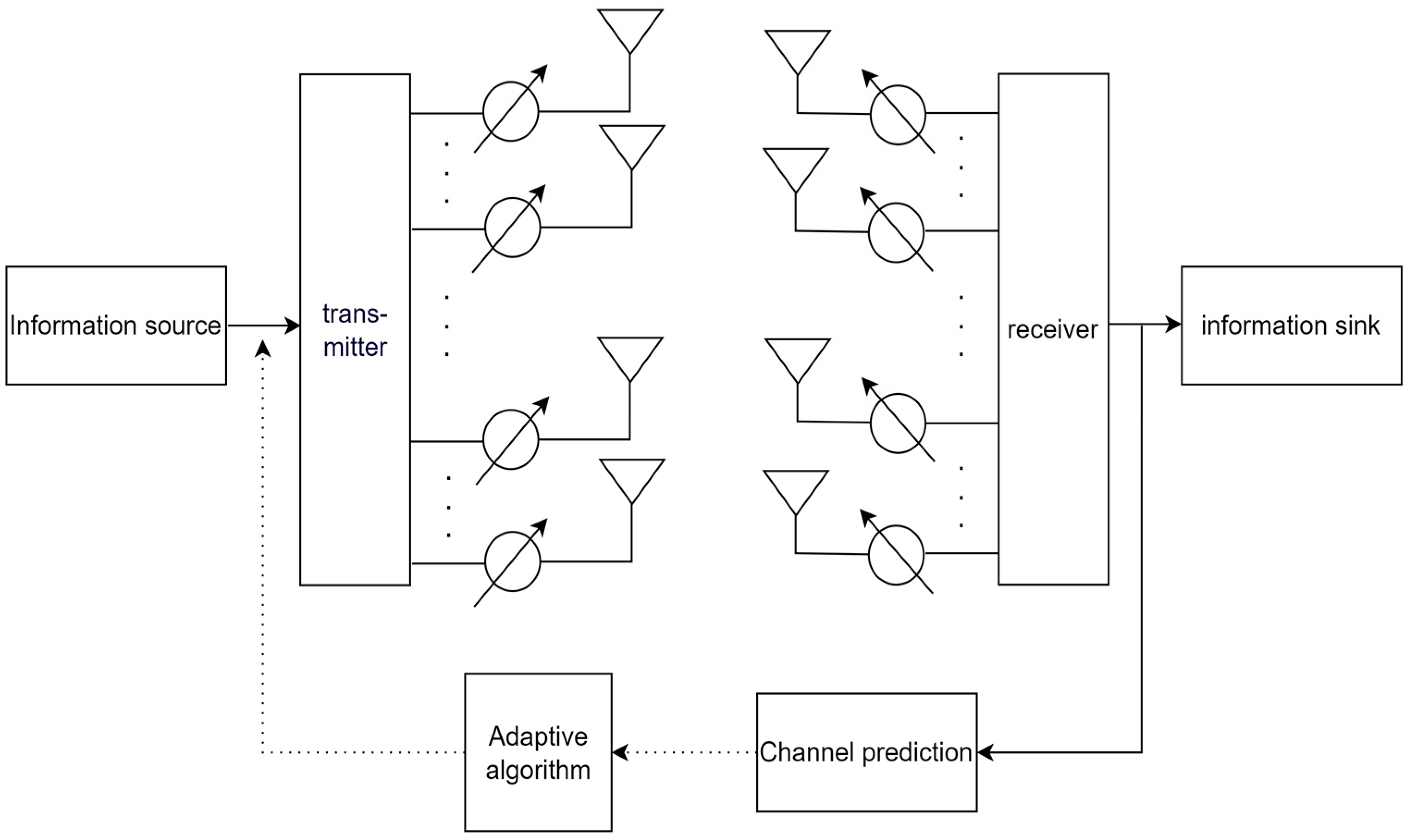
3. System Model
Communication Model
4. SO Improved GRU Model
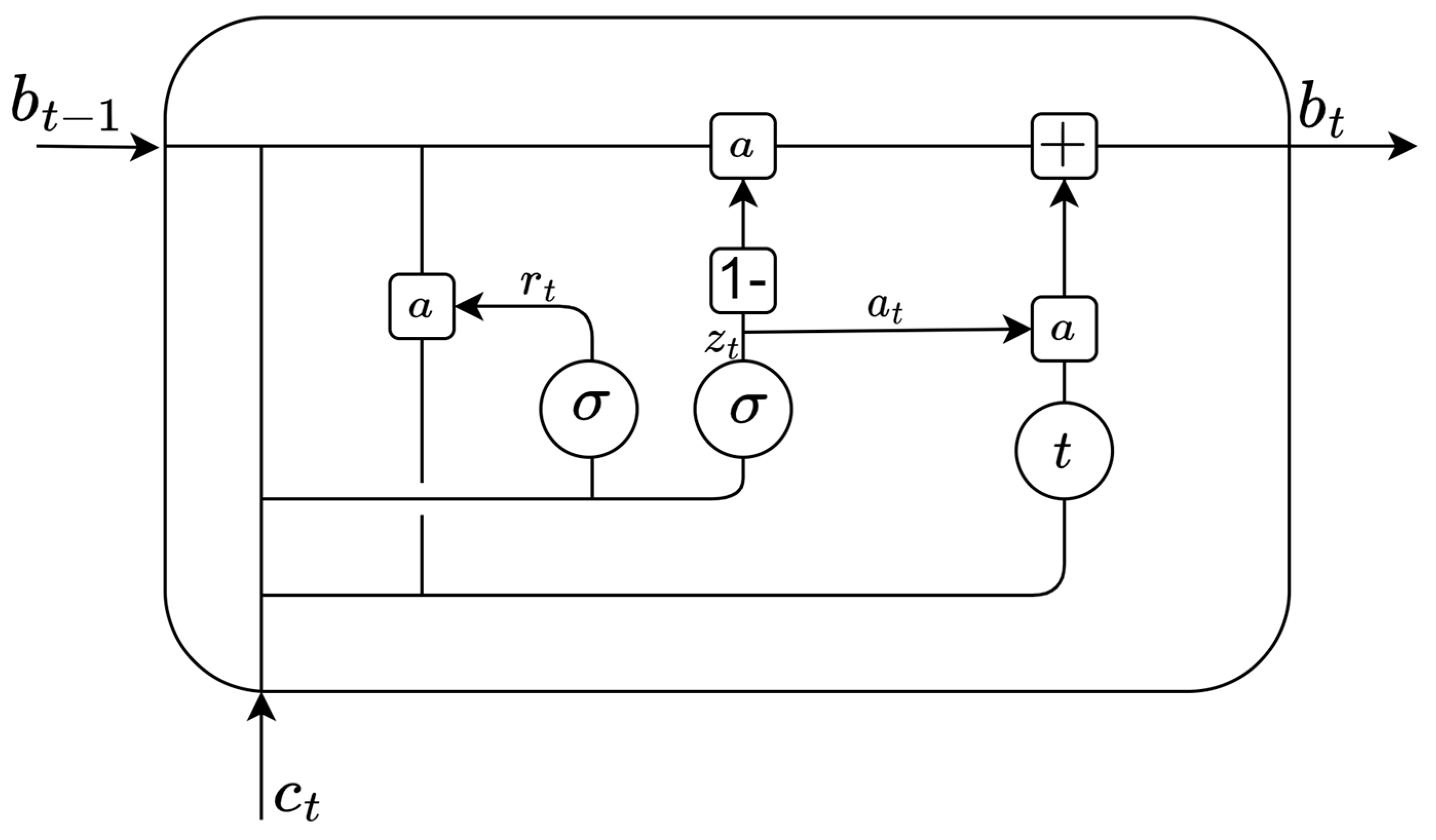
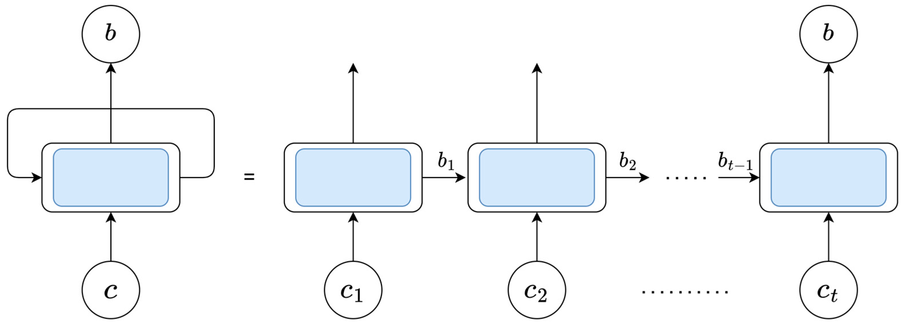
4.1. Gated Recurrent Neural Network
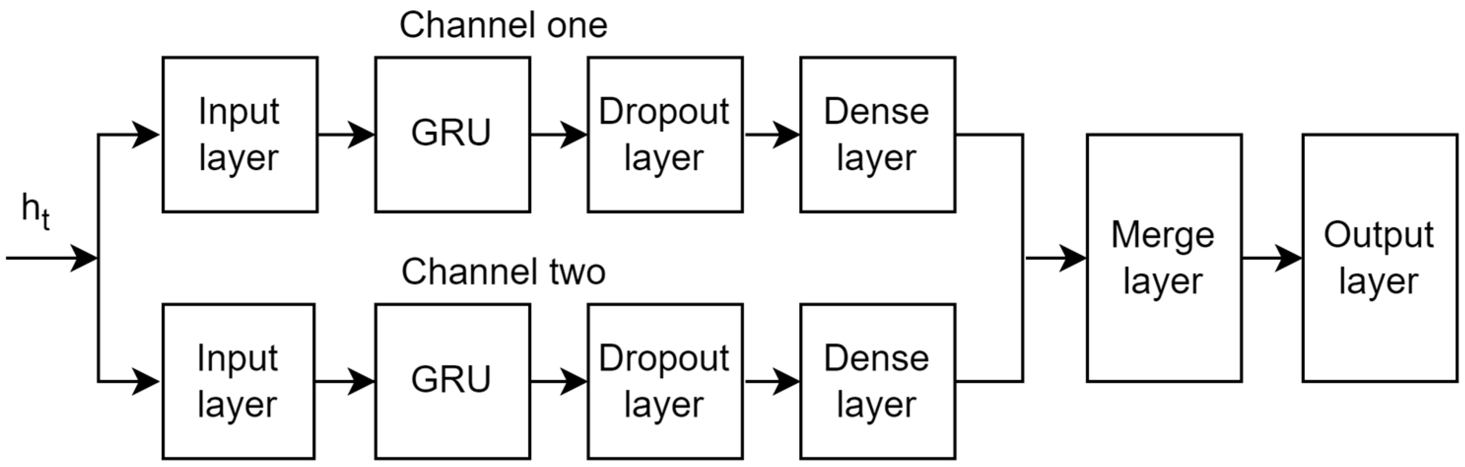
4.2. SO Improved GRU Prediction Model
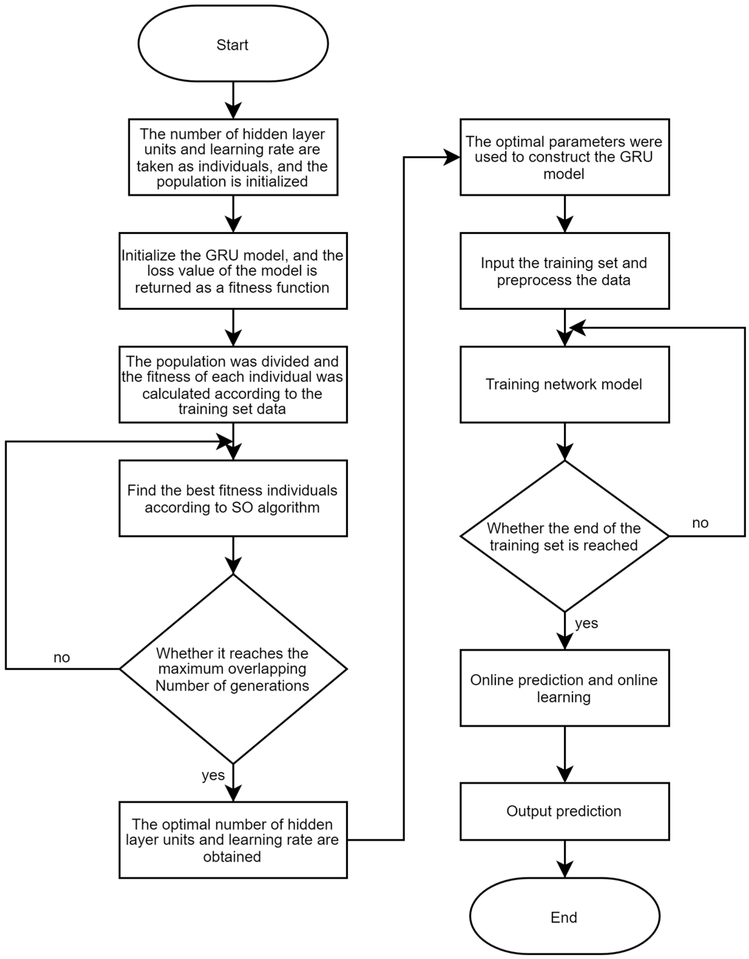
4.3. GRU Algorithm Improved by SO
- Step 1: Build a GRU network model and determine the boundary values of the number of hidden layer units and learning rate according to historical data and inherent model requirements.
- Step 2: Import the training set and preprocess the data.
- Step 3: Determine the number of iterations according to historical experience, initialize the population with boundary values, and divide the female and male populations.
- Step 4: The fitness of everyone is obtained according to the model and training set. The loss value of the network model is used as the fitness function value.
- Step 5: Use the SO algorithm to find the best individual iteration.
- Step 6: Judge whether the SO algorithm reaches the upper limit of iteration times. If yes, retain the final optimal fitness individual and return the optimal number of hidden layer units and learning rate; otherwise, the operation of Step 5 is repeated.
- Step 7: Establish the GRU model with the best parameters, input the pre-processed training set data, and train the network model.
- Step 8: Judge whether it reaches the end of the training set data. If yes, proceed to Step 9; otherwise, continue the training.
- Step 9: Use the trained network model to conduct online prediction and online training.
- Step 10: Output the predicted channel status information.
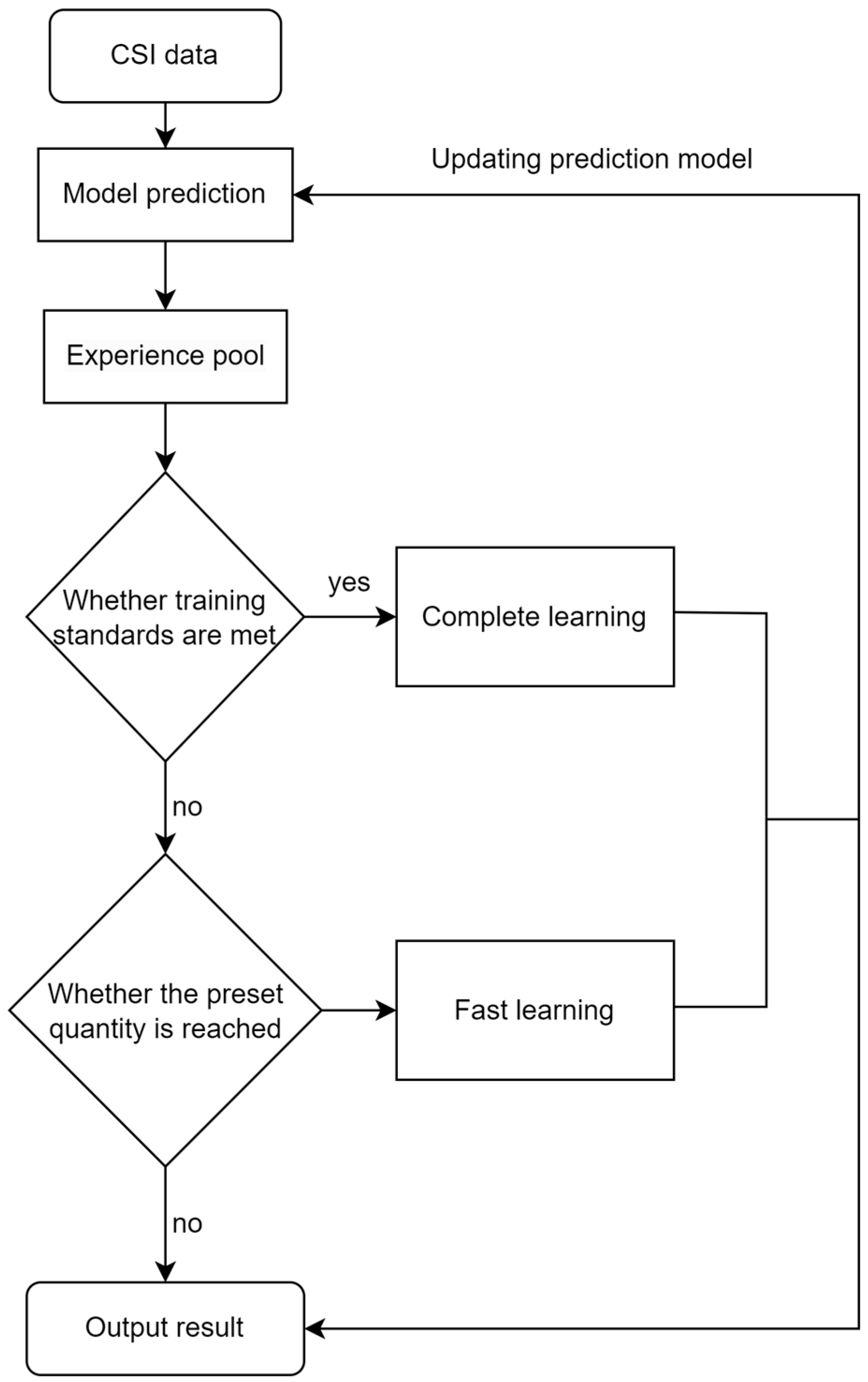
4.4. Model Training and Prediction
| Algorithm 1: Proposed channel predictor |
| 1. Initialize parameters in the SO, such as population M, iteration times T, etc. |
| 2. Use SO to find the optimal parameters. |
| 3. The two-channel GRU model was constructed using the optimal parameters. |
| 4. Start offline Training. |
| 5. While True do |
| 6. Data preprocessing |
| 7. if Total forecast data length > Total data length then |
| 8. end while |
| 9. else |
| 10. i ← 1 |
| 11. while True do |
| 12. if Forecast data length > D then |
| 13. end while |
| 14. end if |
| 15. Single prediction. |
| 16. Store experience in the experience pool. |
| 17. if i % 20 = 0 then |
| 18. Complete learning. |
| 19. else |
| 20. if i % 20 = 0 then |
| 21. Fast learning |
| 22. end if |
| 23. i ← i + 1 |
| 24. end if |
5. Analysis of Simulation Results
5.1. Data Analysis
5.2. Model Parameter Setting and Evaluation Index
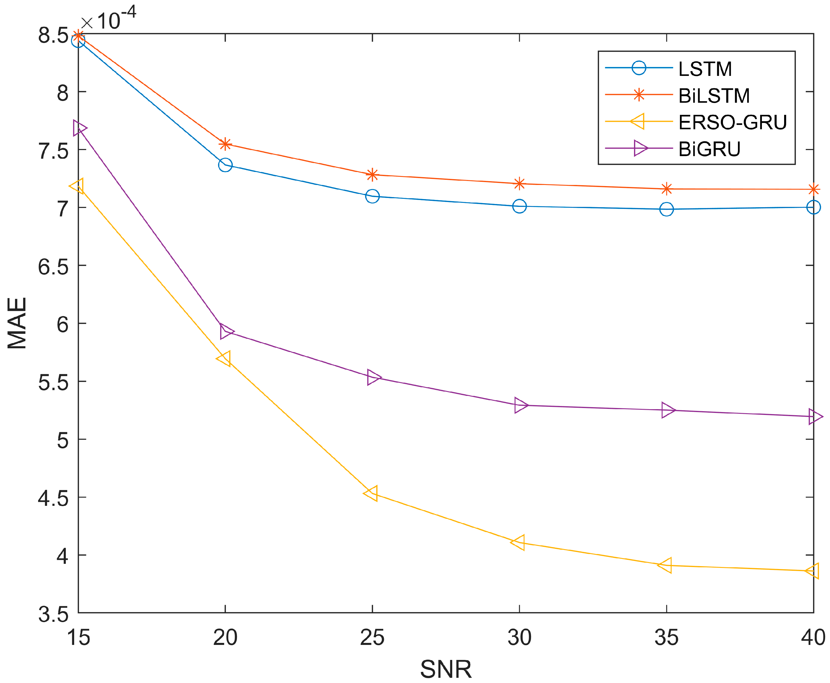
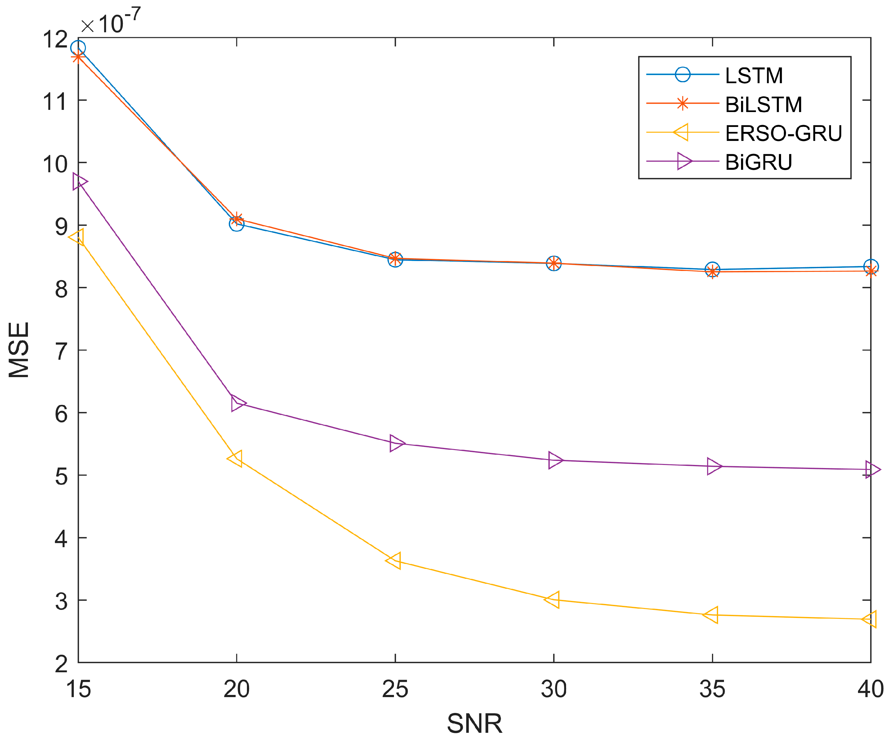
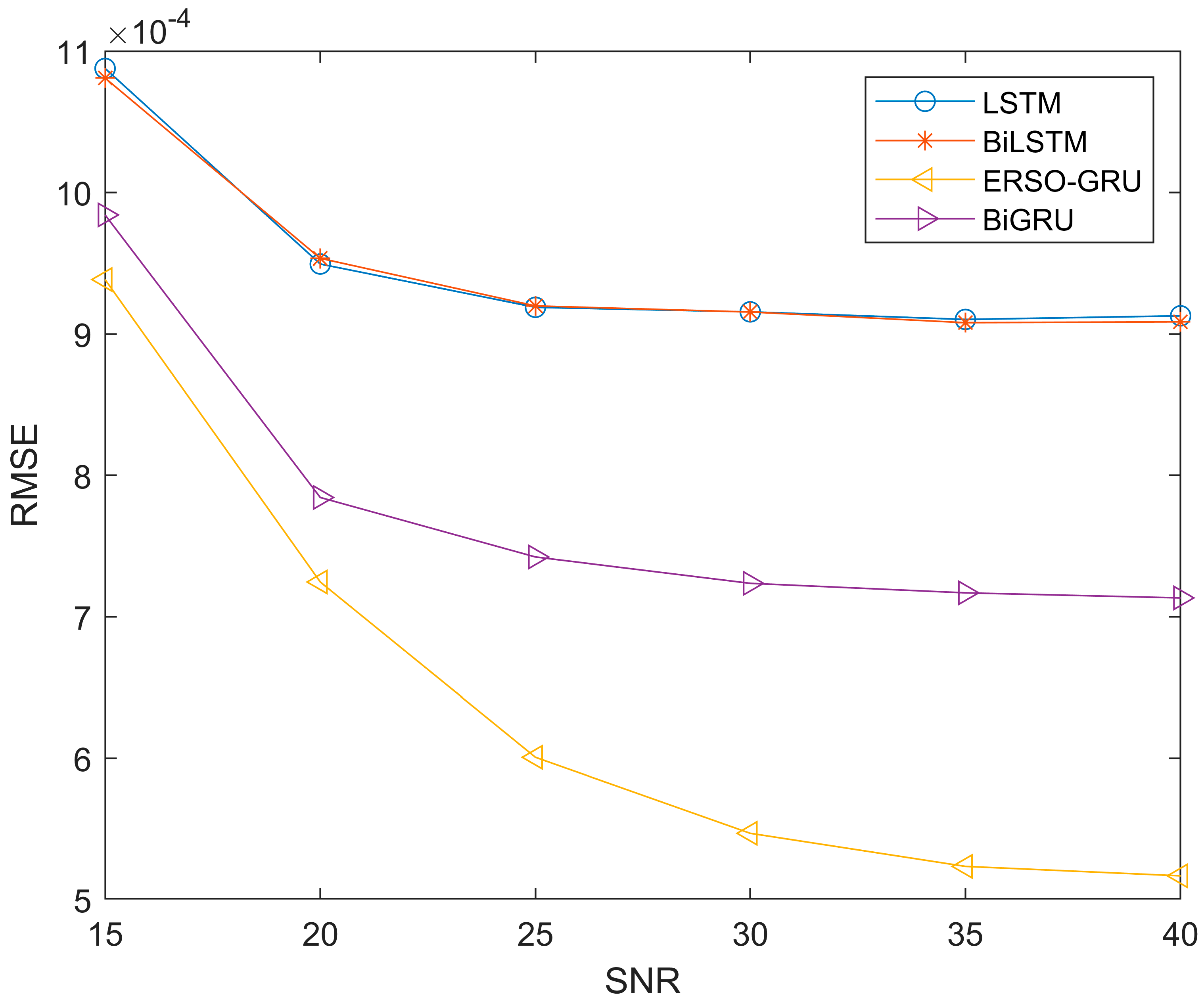
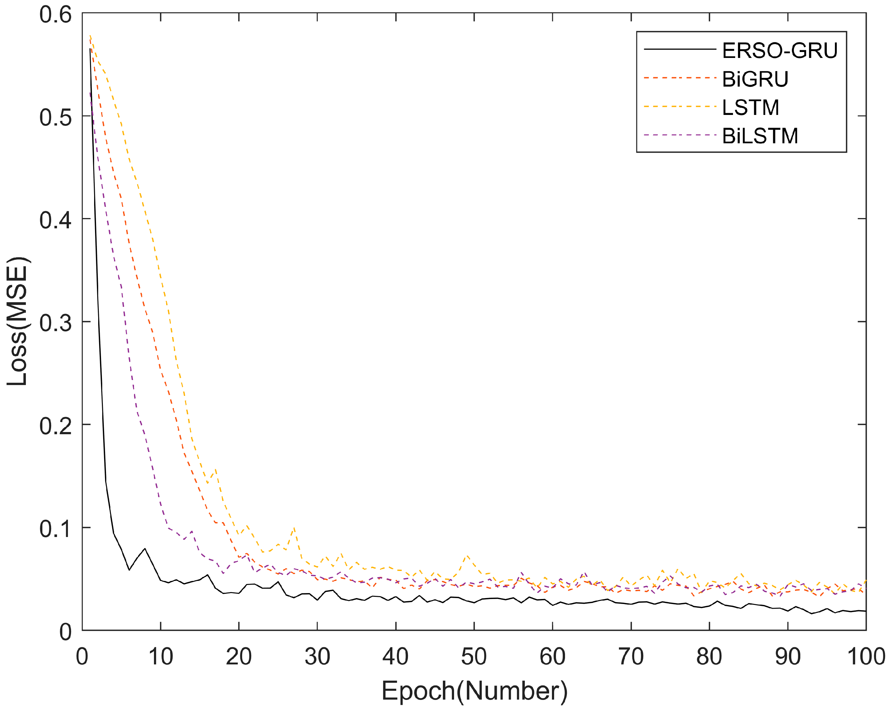
5.3. ERSO Improved GRU Algorithm Performance Analysis
6. Conclusions
Author Contributions
Funding
Institutional Review Board Statement
Informed Consent Statement
Data Availability Statement
Conflicts of Interest
References
- Wang, S.; Lv, T.; Zhang, X.; Lin, Z.; Huang, P. Learning-Based Multi-Channel Access in 5G and Beyond Networks with Fast Time-Varying Channels. IEEE Trans. Veh. Technol. 2020, 69, 5203–5218. [Google Scholar] [CrossRef]
- Agiwal, M.; Kwon, H.; Park, S.; Jin, H. A Survey on 4G-5G Dual Connectivity: Road to 5G Implementation. IEEE Access 2021, 9, 16193–16210. [Google Scholar] [CrossRef]
- Jafri, M.; Srivastava, S.; Venkategowda, N.K.D.; Jagannatham, A.K.; Hanzo, L. Cooperative Hybrid Transmit Beamforming in Cell-free mmWave MIMO Networks. IEEE Trans. Veh. Technol. 2023, 72, 6023–6038. [Google Scholar] [CrossRef]
- Wang, S.; Fu, X.; Ruby, R.; Li, Z. Pilot spoofing detection for massive MIMO mmWave communication systems with a cooperative relay. Comput. Commun. 2023, 202, 33–41. [Google Scholar] [CrossRef]
- Larsson, E.; Edfors, O.; Tufvesson, F.; Marzetta, T. Massive MIMO for next generation wireless systems. IEEE Commun. Mag. 2014, 52, 186–195. [Google Scholar] [CrossRef]
- Ngo, K.-H.; Yang, S.; Guillaud, M.; Decurninge, A. Joint constellation design for the two-user non-coherent multiple-access channel. arXiv 2020, arXiv:2001.04970. [Google Scholar]
- Baeza, V.M.; Armada, A.G. User Grouping for Non-Coherent DPSK Massive SIMO with Heterogeneous Propagation Conditions. In Proceedings of the 2021 Global Congress on Electrical Engineering (GC-ElecEng), Valencia, Spain, 10–12 December 2021; IEEE: Piscataway, NJ, USA, 2021; pp. 26–30. [Google Scholar]
- Lopez-Morales, M.J.; Chen-Hu, K.; Garcia-Armada, A.; Dobre, O.A. Constellation Design for Multiuser Non-Coherent Massive SIMO based on DMPSK Modulation. IEEE Trans. Commun. 2022, 70, 1. [Google Scholar] [CrossRef]
- Duel-Hallen, A. Fading channel prediction for mobile radio adaptive transmission systems. Proc. IEEE 2007, 95, 2299–2313. [Google Scholar] [CrossRef]
- Duel-Hallen, A.; Hu, S.; Hallen, H. Long-range prediction of fading signals. Signal Process. Mag. IEEE 2000, 17, 62–75. [Google Scholar] [CrossRef]
- Chen, J.; Ge, X.; Ni, Q. Coverage and Handoff Analysis of 5G Fractal Small Cell Networks. IEEE Trans. Wirel. Commun. 2019, 18, 1263–1276. [Google Scholar] [CrossRef]
- Raslan, W.A.; Mohamed, M.A.; Abdel-Atty, H.M. Deep-BiGRU based channel estimation scheme for MIMO–FBMC systems. Phys. Commun. 2022, 51, 101592. [Google Scholar] [CrossRef]
- Jiang, W.; Schotten, H.D. Deep Learning for Fading Channel Prediction. IEEE Open J. Commun. Soc. 2020, 1, 320–332. [Google Scholar] [CrossRef]
- Yamak, P.T.; Yujian, L.; Gadosey, P.K. A Comparison between ARIMA, LSTM, and GRU for Time Series Forecasting. In Proceedings of the 2019 2nd International Conference on Algorithms, Computing and Artificial Intelligence, Sanya, China, 20–22 December 2019. [Google Scholar]
- Wang, J.Q.; Du, Y.; Wang, J. LSTM based long-term energy consumption prediction with periodicity. Energy 2020, 197, 117197. [Google Scholar] [CrossRef]
- Zhu, Y.; Dong, X.; Lu, T. An Adaptive and Parameter-Free Recurrent Neural Structure for Wireless Channel Prediction. IEEE Trans. Commun. 2019, 67, 8086–8096. [Google Scholar] [CrossRef]
- LIN, L.-J. Self-improving reactive agents based on reinforcement learning, planning and teaching. Mach. Learn. 1992, 8, 293–321. [Google Scholar] [CrossRef]
- Hashim, F.A.; Hussien, A.G. Snake Optimizer: A novel meta-heuristic optimization algorithm. Knowl. Based Syst. 2022, 242, 108320. [Google Scholar] [CrossRef]
- Liao, R.; Wen, H.; Wu, J.; Song, H.; Pan, F.; Dong, L. The Rayleigh Fading Channel Prediction via Deep Learning. Wirel. Commun. Mob. Comput. 2018, 2018, 6497340. [Google Scholar] [CrossRef]
- Jiang, W.; Schotten, H.D. Neural Network-Based Fading Channel Prediction: A Comprehensive Overview. IEEE Access 2019, 7, 118112–118124. [Google Scholar] [CrossRef]
- Mahjoub, S.; Chrifi-Alaoui, L.; Marhic, B.; Delahoche, L. Predicting Energy Consumption Using LSTM, Multi-Layer GRU and Drop-GRU Neural Networks. Sensors 2022, 22, 4062. [Google Scholar] [CrossRef]
- Jiang, W.; Schotten, H.D. Recurrent neural networks with long short-term memory for fading channel prediction. In Proceedings of the 2020 IEEE 91st Vehicular Technology Conference (VTC2020-Spring), Antwerp, Belgium, 25–28 May 2020; IEEE: Piscataway, NJ, USA, 2020; pp. 1–5. [Google Scholar]
- Jiang, W.; Schotten, H.D. A deep learning method to predict fading channel in multi-antenna systems. In Proceedings of the 2020 IEEE 91st Vehicular Technology Conference (VTC2020-Spring), Antwerp, Belgium, 25–28 May 2020; IEEE: Piscataway, NJ, USA, 2020; pp. 1–5. [Google Scholar]
- Mattu, S.R.; Theagarajan, L.N.; Chockalingam, A. Deep Channel Prediction: A DNN Framework for Receiver Design in Time-Varying Fading Channels. IEEE Trans. Veh. Technol. 2022, 71, 6439–6453. [Google Scholar] [CrossRef]
- Chen, F.-J.; Kwong, S.; Kok, C.-W. Blind MMSE Equalization of SISO IIR Channels Using Oversampling and Multichannel Linear Prediction. IEEE Trans. Veh. Technol. 2017. early access. [Google Scholar] [CrossRef]
- Patil, S.A.; Raj, L.A.; Singh, B.K. Prediction of IoT Traffic Using the Gated Recurrent Unit Neural Network- (GRU-NN-) Based Predictive Model. Secur. Commun. Netw. 2021, 2021, 1425732. [Google Scholar] [CrossRef]
- Yan, J.; Liu, J.; Yu, Y.; Xu, H. Water Quality Prediction in the Luan River Based on 1-DRCNN and BiGRU Hybrid Neural Network Model. Water 2021, 13, 1273. [Google Scholar] [CrossRef]
- NIST. Networked Control Systems Group—Measurement Data Files. 2017. Available online: https://www.nist.gov/ctl/smart-connected-systems-division/networked-control-systems-group/measurement-data-files (accessed on 18 November 2022).
- AlHajri, M.I.; Ali, N.T.; Shubair, R.M. 4 GHz Indoor Channel Measurements Data Set. November 2018. Available online: https://ieee-dataport.org/documents/24-ghz-indoor-channel-measurements (accessed on 18 November 2022).


| ERSO-GRU | Value Range |
|---|---|
| Snake populations M | 10 |
| Maximum iterations T | 100 |
| Hidden layer units one | [1, 50] |
| Hidden layer units two | [1, 50] |
| Learning rate | [0.00001, 0.5] |
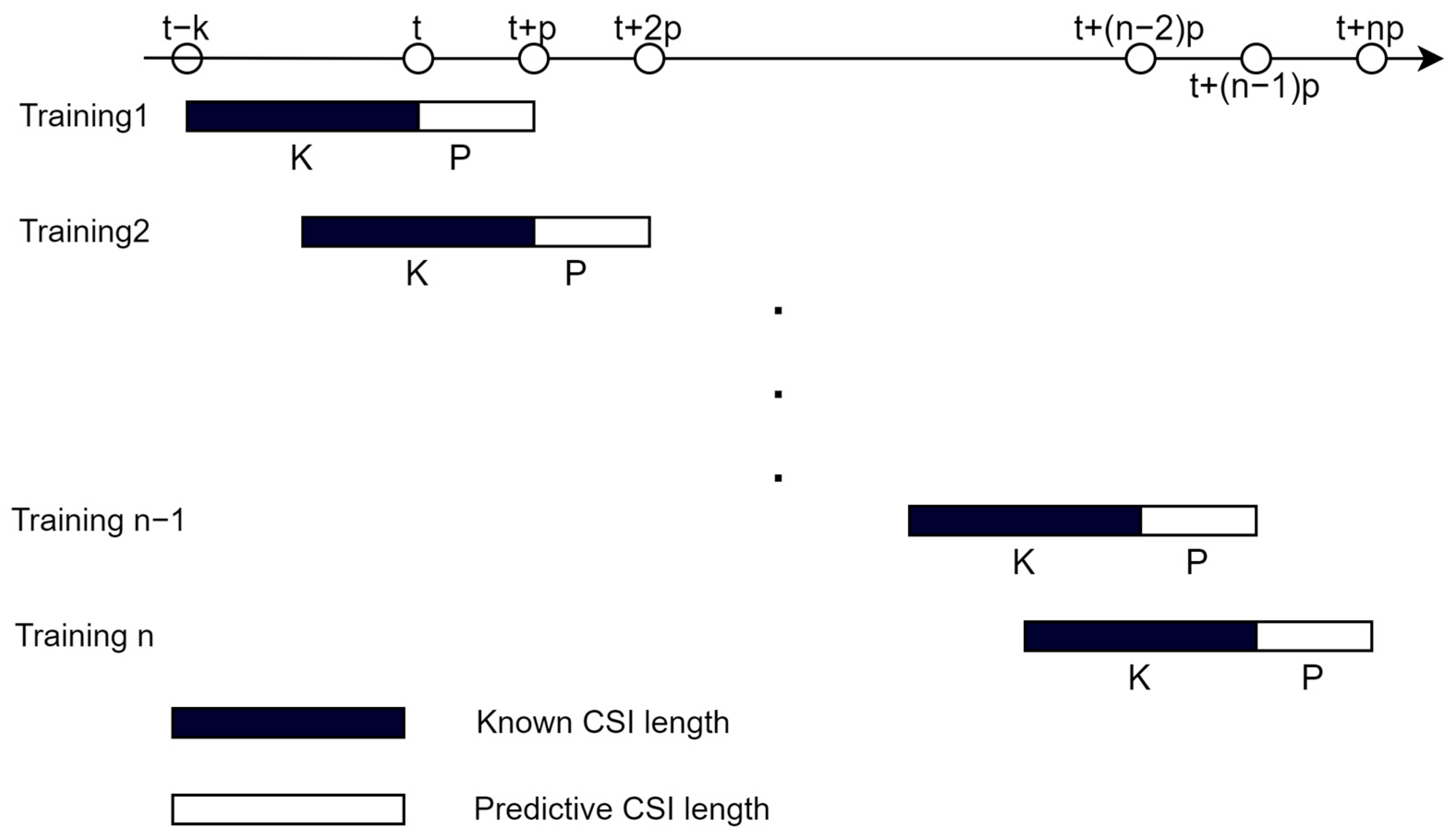
| Known CSI length K | 30 |
| Predicted CSI length P | 10 |
| Data block size | 200 |
| Experience pool size | 200 |
| Evaluation Criteria | Definition | Formula |
|---|---|---|
| MAE | Mean absolute error | |
| MAPE | Mean absolute percentage error | |
| MSE | Mean square error | |
| RMSE | Root mean square error |
| Locations | Model | MAE | MAPE | MSE | RMSE |
|---|---|---|---|---|---|
| Lab139 | LSTM | 5.9804 × 10⁻⁴ | 1.3983 | 6.6456 × 10⁻⁷ | 8.1437 × 10⁻⁴ |
| BiLSTM | 6.8622 × 10⁻⁴ | 1.6185 | 8.1333 × 10⁻⁷ | 8.9885 × 10⁻⁴ | |
| BiGRU | 4.7453 × 10⁻⁴ | 1.1571 | 4.1525 × 10⁻⁷ | 6.4409 × 10⁻⁴ | |
| ERSO-GRU | 3.4329 × 10⁻⁴ | 0.7859 | 2.5012 × 10⁻⁷ | 4.9732 × 10⁻⁴ | |
| Corridor_rm155 | LSTM | 6.8724 × 10⁻⁴ | 1.4415 | 7.1536 × 10⁻⁷ | 8.4559 × 10⁻⁴ |
| BiLSTM | 7.0936 × 10⁻⁴ | 1.5649 | 7.5727 × 10⁻⁷ | 8.6966 × 10⁻⁴ | |
| BiGRU | 4.7949 × 10⁻⁴ | 0.7473 | 3.8292 × 10⁻⁷ | 6.1840 × 10⁻⁴ | |
| ERSO-GRU | 4.0665 × 10⁻⁴ | 0.6846 | 3.1759 × 10⁻⁷ | 5.6068 × 10⁻⁴ | |
| Main_Lobby | LSTM | 6.1129 × 10⁻⁴ | 4.0924 | 6.4957 × 10⁻⁷ | 8.0544 × 10⁻⁴ |
| BiLSTM | 6.8232 × 10⁻⁴ | 5.7196 | 8.1423 × 10⁻⁷ | 9.0118 × 10⁻⁴ | |
| BiGRU | 4.3570 × 10⁻⁴ | 2.8235 | 3.5520 × 10⁻⁷ | 5.9579 × 10⁻⁴ | |
| ERSO-GRU | 3.6049 × 10⁻⁴ | 2.1537 | 2.5163 × 10⁻⁷ | 4.9942 × 10⁻⁴ | |
| Sports_Hall | LSTM | 6.5955 × 10⁻⁴ | 1.2397 | 8.5151 × 10⁻⁷ | 9.2237 × 10⁻⁴ |
| BiLSTM | 6.7640 × 10⁻⁴ | 1.2836 | 8.5660 × 10⁻⁷ | 9.2524 × 10⁻⁴ | |
| BiGRU | 4.6952 × 10⁻⁴ | 0.9228 | 4.4041 × 10⁻⁷ | 6.6353 × 10⁻⁴ | |
| ERSO-GRU | 3.7218 × 10⁻⁴ | 0.6650 | 2.7051 × 10⁻⁷ | 5.1950 × 10⁻⁴ |
Disclaimer/Publisher’s Note: The statements, opinions and data contained in all publications are solely those of the individual author(s) and contributor(s) and not of MDPI and/or the editor(s). MDPI and/or the editor(s) disclaim responsibility for any injury to people or property resulting from any ideas, methods, instructions or products referred to in the content. |
© 2023 by the authors. Licensee MDPI, Basel, Switzerland. This article is an open access article distributed under the terms and conditions of the Creative Commons Attribution (CC BY) license (https://creativecommons.org/licenses/by/4.0/).
Share and Cite
Liu, Q.; Wang, P.; Sun, J.; Li, R.; Li, Y. Wireless Channel Prediction of GRU Based on Experience Replay and Snake Optimizer. Sensors 2023, 23, 6270. https://doi.org/10.3390/s23146270
Liu Q, Wang P, Sun J, Li R, Li Y. Wireless Channel Prediction of GRU Based on Experience Replay and Snake Optimizer. Sensors. 2023; 23(14):6270. https://doi.org/10.3390/s23146270
Chicago/Turabian StyleLiu, Qingli, Peiling Wang, Jiaxu Sun, Rui Li, and Yangyang Li. 2023. "Wireless Channel Prediction of GRU Based on Experience Replay and Snake Optimizer" Sensors 23, no. 14: 6270. https://doi.org/10.3390/s23146270
APA StyleLiu, Q., Wang, P., Sun, J., Li, R., & Li, Y. (2023). Wireless Channel Prediction of GRU Based on Experience Replay and Snake Optimizer. Sensors, 23(14), 6270. https://doi.org/10.3390/s23146270