Abstract
Due to the increase in the number of mobile stations in recent years, cooperative relaying systems have emerged as a promising technique for improving the quality of fifth-generation (5G) wireless networks with an extension of the coverage area. In this paper, we propose a two-hop orthogonal frequency division multiplexing and code-division multiple-access (OFDM-CDMA) multiple-input multiple-output (MIMO) relay system, which combines, both at the source and relay nodes, a tensor space–time–frequency (TSTF) coding with a multiple symbol matrices Kronecker product (MSMKron), called TSTF-MSMKron coding, aiming to increase the diversity gain. It is first established that the signals received at the relay and the destination satisfy generalized Tucker models whose core tensors are the coding tensors. Assuming the coding tensors are known at both nodes, tensor models are exploited to derive two semi-blind receivers, composed of two steps, to jointly estimate symbol matrices and individual channels. Necessary conditions for parameter identifiability with each receiver are established. Extensive Monte Carlo simulation results are provided to show the impact of design parameters on the symbol error rate (SER) performance, using the zero-forcing (ZF) receiver. Next, Monte Carlo simulations illustrate the effectiveness of the proposed TSTF-MSMKron coding and semi-blind receivers, highlighting the benefit of exploiting the new coding to increase the diversity gain.
1. Introduction
In recent years, wireless communication systems have experienced great growth in the number of users and new applications such as autonomous vehicles, smart homes, Internet of Things (IoT) and virtual/augmented reality. Compared to fourth-generation (4G) wireless systems, 5G ones offer advantages in terms of data rate, reliability, latency, energy efficiency, and mobility. To fulfill these objectives, 5G needs to operate at high frequency bands, with more base stations in a smaller area, to provide a better reliability and transmission quality to the users [1,2,3].
That explains why in the last few years, cooperative multiple-input multiple-output (MIMO) systems have attracted a lot of attention for 5G mobile networks to increase the transmission coverage area, data rates and performance of wireless communications [4]. Cooperative MIMO systems provide spatial diversity and spatial multiplexing due to the use of multiple antennas to transmit and receive signals at each node of the systems. However, individual channel estimation in a cooperative MIMO system is a fundamental problem to solve, since the reliability of the system greatly depends on the accuracy of channel state information (CSI) in each hop.
During the last two decades, tensor models have been widely used for designing wireless communication systems [5,6]. Tensor-based approaches allow taking different diversities (space, time, frequency, code, polarization, etc.) into account during the system design and developing semi-blind receivers for jointly estimating the channels and symbol matrices under more relaxed conditions than matrix-based methods. Many receivers exploit the two most popular tensor decompositions, namely the Tucker [7] and Parallel Factors Analysis (PARAFAC) [8] models, as in [9,10,11,12,13,14]. However, during the last decade, the design of tensor-based wireless communication systems has led to the development of several new tensor models such as, for instance, the nested PARAFAC [15] and nested Tucker [16] models. See for instance their use in the context of point-to-point MIMO systems [17] and cooperative MIMO systems [18,19,20,21,22].
In the context of cooperative systems, some works are dedicated to the use of a training sequence for estimating the channels in a supervised way, as in [14,23]. Such supervised systems are bandwidth-consuming, which explains the development of semi-blind receivers to jointly estimate the transmitted information symbols and the channels, i.e., without the use of training sequences, such as in the case for the systems briefly introduced below. Many works combine cooperative MIMO systems with different space/time/frequency codings to increase system diversity and obtain better performance in terms of channel and symbol estimation. Among the used codings, one can mention the Khatri–Rao space–time (KRST) coding [18,19,24,25], the multiple Khatri–Rao and Kronecker space–time (MKRST and MKronST) codings [17,26], the tensor space–time (TST) [27,28,29] and tensor–space–time–frequency (TSTF) codings [30]. Depending on the coding chosen for the relay system, different tensor models are obtained for the signals received at the relay and destination nodes. An exploitation of these models makes it possible to derive two families of receivers. One is made up of the most common receivers based on iterative algorithms such as alternating least squares (ALS) or the Levenbergh–Marquardt (LM) method. The other is composed of closed-form algorithms based on singular value decomposition (SVD) calculation, such as Khatri–Rao and Kronecker factorization algorithms, which are denoted KRF and KronF respectively.
In Table 1, the tensor-based MIMO cooperative systems of the above cited references are compared in terms of system type (number of hops), coding, tensor model, and receiver, with the proposed MIMO relay system, which is referenced as “New” in Table 1.

Table 1.
Tensor-based MIMO cooperative systems.
We now briefly comment on the relay systems compared in Table 1 from a historical perspective. First, it is important to note that all these systems consider an amplify-and-forward (AF) protocol at the relays except the system in [26] for which the AF protocol is compared with the decode-and-forward (DF) and estimate-and-forward (EF) ones, showing that the use of these last two protocols allows significantly improving the SER performance at the cost of an additional computational complexity at the relay. From a coding point of view, the Khatri–Rao space–time (KRST) coding was firstly used in [18,19,24] for a two-hop system and then in [25] for a multi-hop system. In [22], KRST coding is combined with a rotation coding matrix for a three-hop system.
The tensor space–time (TST) coding initialy proposed in [27], in the context of point-to-point systems, was used for a two-hop system in [16], leading to a new tensor model called nested Tucker decomposition (TD) and then for a multi-hop system in [21]. In this last reference, a new tensor model called high-order nested Tucker decomposition (HONTD) was introduced. In [28], TST coding is used in a two-hop multi-relay system where the relays directly and sequentially communicate with the destination node. The sequential transmission from the relays to the destination leads to a new coupled nested TD model. In [29], TST coding is combined with a PARAFAC coding structure for a two half-duplex relays system. Two new codings, denoted MKRST and MKronST, were proposed in [26] for a two-hop system, leading to a nested PARAFAC model for the tensor of signals received at destination which is exploited to develop closed-form semi-blind receivers for joint symbol and channel estimation.
An important difference between the systems in Table 1 and the system presented in this paper concerns the a priori information needed to eliminate scaling ambiguities. Thus, our system only requires a priori knowledge of one entry of the symbol matrices, whereas all the systems in Table 1 also require knowledge of one entry or of one row of the channel matrices, which is a much more restrictive assumption.
This paper proposes a new two-hop OFDM-CDMA MIMO relay system which combines a tensor space–time–frequency (TSTF) coding with a multiple Kronecker product of symbol matrices (MSMKron) at the source and relay nodes. This new coding scheme, called TSTF-MSMKron coding, can be viewed as a generalization of the codings proposed in [26,30], with the aim of increasing the diversity gain. It is established that the signals received at the relay and destination nodes satisfy generalized Tucker models whose core tensors are the coding tensors. Assuming the coding tensors are known at both nodes, the multilinear structure of tensor models is exploited to derive two semi-blind receivers for jointly estimating the symbol matrices and individual channels. Necessary conditions for parameter identifiability with each receiver are established. Extensive Monte Carlo simulations illustrate the effectiveness of the proposed TSTF-MSMKron coding and semi-blind receivers. Note that our two-hop MIMO relay system differs mainly from the systems compared in Table 1 by the proposed TSTF-MSMMKron coding scheme which induces a greater diversity gain than the codings used by the systems referenced in Table 1. Another important difference lies in the consideration of frequency-dependent channels, i.e., three-dimensional channels. These assumptions lead to received signal tensors at the relay and the destination that satisfy generalized Tucker models whose essential uniqueness is ensured by the a priori knowledge of coding tensors. Scalar ambiguities can be eliminated assuming the knowledge of only one symbol per each symbol matrix. Exploiting the tensor models of received signals allows developing two types of semi-blind receivers for estimating the information symbols and the individual channels: one is iterative based on the Bi-ALS algorithm to estimate each individual channel and the Kronecker product of symbol matrices, combined with the KronF method to separate the symbol matrices, while the other one is closed form and based on the THOSVD algorithm [31], which allows simultaneously estimating each individual channel and symbol matrix. Note that unlike almost all relay systems existing in the literature which use the AF protocol, the proposed two-hop system uses the DF protocol at the relay, which greatly facilitates its generalization to the multi-hop case.
The main contributions of the paper can be summarized as follows:
- A new two-hop OFDM-CDMA system that combines a TSTF coding with a multiple Kronecker product of symbol matrices (MSMKron) at the source and relay nodes is proposed.
- It is established that the tensor of signals received at each hop satisfies a generalized Tucker model.
- By exploiting the tensor model of the signals received at the relay and destination nodes, two semi-blind receivers are derived to jointly estimate the individual source–relay and relay–destination channels and transmitted symbols.
- System model uniqueness and parameter identifiability conditions for each proposed receiver are analyzed.
- The performance of the TSTF-MSMKron coding and the impact of design parameters on the symbol error rate (SER) are first evaluated using the zero-forcing (ZF) receiver, i.e., under the assumption of a perfect channel knowledge, by means of extensive Monte Carlo simulations. Then, the proposed semi-blind receivers are compared for symbol and channel estimation.
The rest of the paper is organized as follows. Section 2 presents tensor preliminaries. Section 3 first describes the system model, presenting the TSTF-MSMKron coding and the signals received at the relay and destination. These signals form two tensors that satisfy generalized Tucker decompositions. In Section 4, two semi-blind receivers are proposed to jointly estimate the symbol matrices and channels. Necessary conditions for parameter identifiability are derived for each receiver. In Section 6, extensive Monte Carlo simulation results are provided to illustrate the effectiveness of the proposed two-hop relay system. Section 7 concludes the paper.
Notation: scalars, column vectors, matrices, and tensors are denoted by lowercase, boldface lowercase, boldface uppercase and boldface calligraphic letters, e.g., x, , X, and , respectively. The transpose, complex conjugate, complex conjugate transpose, and Moore–Penrose pseudo-inverse of are represented by , and , respectively. We denote by the element and by (resp. ) the ith row (resp. jth column) of . The (, …, ) element of the N-order tensor will be written . and represent the identity matrix of size and the identity tensor of N-order and size , respectively. denotes an estimate of and represents the matrix after ambiguities suppression.
represents an unfolding of the third-order tensor of dimension . The vec and unvec operators are defined by . By slicing the third-order tensor along each mode, we obtain three types of matrix slices called horizontal, lateral, and frontal slices, which are denoted, respectively, as follows:
All acronyms used in the paper are summarized after Section 7.
2. Tensor Preliminaries
The mode-n product between a tensor and a matrix , denoted by , gives an N-order tensor of size , which is defined by:
The mode-n product between two tensors and is denoted by , with . This product gives an N-order tensor , which is defined as [30]:
The sum is over the second index of the tensor , as for the mode-n product (1) between a tensor and a matrix. For example, consider the third-order tensors and . The mode-1 product is given by:
We now introduce the notion of a generalized Tucker-() model for an N-order tensor , with , which is defined as [32,33]:
where is an ordered subset of the set . This model can be written in terms of mode-n products as:
where is the core tensor, and are tensor factors for , where is a subset of . For example, let us consider two factors, where the first one is a third-order tensor and the second one is a matrix . A generalized Tucker-() model is given by:
where . In scalar form, Equation (6) can be written as:
3. System Model
3.1. Presentation of the Proposed Two-Hop System
Consider a two-hop MIMO OFDM-CDMA system, as illustrated in Figure 1. This system is equipped with , and antennas at the source, relay and destination nodes, respectively. The source–relay () and relay–destination () channels are assumed to be flat Rayleigh fading, which is represented by third-order tensors whose coefficients are zero-mean circularly symmetric complex Gaussian i.i.d. (independent and identically distributed) random variables that are constant during at least P transmission blocks.
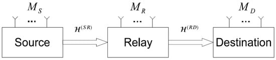
Figure 1.
Block diagram of the two-hop MIMO relay system.
The decode-and-forward (DF) protocol is considered at the relay, and the transmission occurs in two hops. During the first one, the coded symbols are transmitted by the source to the relay via the channel and decoded at the relay. During the second one, the estimated symbols are re-encoded and then re-transmitted by the relay to the destination via the channel . Each symbol matrix , with , for , is composed of data streams, each one containing information symbols. The transmission protocol is detailed in the next section which defines the TSTF-MSMKron coding. Then, in Section 3.3 and Section 3.4, the tensors of signals received at the relay and the destination will be described, respectively.
3.2. TSTF-MSMKron Coding
In the proposed relay system, the coding at the source node is composed of two steps. During the first one, a multiple Kronecker product of L symbol matrices is calculated as:
where , and . The scalar form of (8) is:
with , and , where and denote the indices and in . This operation, called MSMKron coding, corresponds to a simplified version of the MKronST coding [26] without a known precoding matrix. This coding induces time and code spreadings of each symbol due to the multiple Kronecker product of the symbol matrix with the other matrices , and .
The transmission being composed of P time-slots means each symbol is repeated times, which implies an increase of time and code diversities when increasing the dimensions and , respectively.
During the second step, the MSMKron coding is combined with a tensor space–time–frequency (TSTF) coding [30] carried out by means of the (L+3)-order tensor in such a way that the tensor of signals coded at the source satisfies an (L+3)-order Tucker model given by:
Note that the core tensor of this decomposition is the coding tensor . In scalar notation, the coded signals transmitted by the antenna at the source, using the subcarrier, during the time slot are given by:
where . The TSTF-MSMKron coding increases space–time–frequency diversity, as will be illustrated in the simulations.
3.3. Tensor of Signals Received at the Relay
In the noise-free case and assuming a flat Rayleigh fading propagation channel, the signal received at the antenna of the relay, during the symbol period of the block and associated with the subcarrier, is given by:
where and is an entry of the channel . In terms of mode-n products, we have:
Note that the transmission via channel can be interpreted as a mode-1 linear transformation applied to the tensor of coded signals. Substituting (11) into (12) gives the signal received at the relay written in scalar form as:
The signals received at the relay form the tensor that satisfies a generalized Tucker-() model given by:
where represents the symbol matrices encoded by the TSTF-MSMKron coding for , and is the core tensor of the Tucker model. As is well known, knowledge of the core tensor implies the uniqueness of this model. Combining modes 2 to of tensors and results in contracted forms and , and Equation (15) can be rewritten as:
From the Tucker model (16), it is easy to deduce the following matrix unfoldings of the tensor :
with and previously defined in the notation. Note that the identity matrix in (17) is associated with repetitions of the symbol matrices inducing time-frequency diversity for the system.
The block structure of the matrix unfoldings and in Equations (17) and (19), respectively, is defined as follows:
in (20) is a block-diagonal matrix, formed of F diagonal blocks of dimension , each block being formed of column vectors corresponding to a vectorized form of the tensor slice of size , for , such that . Similarly, in (21) is a block-diagonal matrix whose diagonal blocks are of dimension , with .
To illustrate the matrix unfolding (21), consider the case where , leading to the following matrix:
3.4. Tensor of Signals Received at the Destination
With the DF protocol, the symbols received at the relay are first decoded by means of one of the receivers described in Section 4, leading to the estimated symbol matrices , which are also written as . The estimated symbols are then re-encoded at the relay using a TSTF-MSMKron coding, with the tensor coding . The re-encoded signals are transmitted by the relay to the destination via the channel . The signals received at the destination are similar to the signals received at the relay, defined by Equations (14) and (15), with the following correspondences:
Similar to (14), in the noiseless case, the signal received at the antenna of the destination node, during the symbol period of the time block and associated with the subcarrier, is given by:
and the generalized Tucker-() model (15) becomes:
where . Matrix unfoldings of this tensor can be deduced from (17)–(19) using the correspondences (23) and (24) with , and instead of , and , respectively.
The proposed OFDM-CDMA relaying system is illustrated by means of the block diagram in Figure 2.
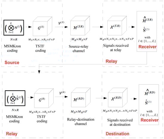
Figure 2.
Block diagram of the proposed two-hop MIMO OFDM-CDMA communication system.
The system design parameters and the definitions of the system matrices and tensors are summarized in Table 2 and Table 3, respectively.
Table 2.
System design parameters.
Table 3.
System matrices and tensors.
4. Semi-Blind Receivers
In this section, two semi-blind receivers are proposed to estimate the channel tensors and symbol matrices at the relay and destination nodes. We assume that the coding tensors and are known. We also assume that one symbol of each symbol matrix is known to eliminate scalar ambiguities. The symbol matrices and the channel tensor are estimated at the relay, while the symbol matrices and the channel tensor are estimated at the destination. The proposed receivers are detailed for the relay. The same receivers can be derived for the destination, using the correspondences (23) and (24). The first one is based on the alternating least squares (ALS) algorithm to estimate the channel and the Kronecker product of symbol matrices, which is followed by the Kronecker factorization (KronF) method to separate the symbol matrices, while the second one is a closed-form solution allowing to jointly estimate the channel and the symbol matrices by means of the truncated higher-order singular value decomposition (THOSVD) algorithm.
4.1. Bi-ALS-KronF Receiver
In the first step, the bi-alternating least squares (Bi-ALS) algorithm is used to jointly estimate the MSMKron product and the channel tensor . Then, the KronF algorithm is applied to separate the symbol matrices. The Bi-ALS algorithm results from the minimization of the following cost function deduced from Equation (16):
where is the Frobenius norm. The Bi-ALS method replaces the optimization problem (27) by two LS sub-problems deduced from the matrix unfoldings (17) and (18), leading to the alternate minimization of the following LS criteria:
The update equations at iteration are given by:
The matrices and must have full column rank to ensure the uniqueness of the LS estimates, which implies the following necessary conditions: and .
To simplify the computation of the estimate in Equation (30), we assume that the matrices and have full column rank, which implies: and , respectively. Moreover, to simplify the computation of in Equation (31), we assume that the unfolding is chosen as a full column rank truncated DFT matrix, which allows us to replace its pseudo-inverse by its transconjugate, implying the necessary condition: . We also assume that has full column rank, implying . Exploiting these assumptions and substituting the unfolding by Equation (20) simplifies the LS estimates (30) and (31) as:
The Bi-ALS algorithms (32) and (33) are simplified versions of (30) and (31) in terms of pseudo-inverses computation at the price of additional constraints on the design parameters.
The error at the iteration, deduced from (17), is considered for deciding the convergence of the Bi-ALS algorithm:
Convergence at the iteration is declared when this error does not significantly change between two successive iterations, i.e., , where is a predefined threshold. Since the core tensor is assumed to be known, there is no permutation ambiguity, and the generalized Tucker model (16) is unique up to scalar scaling ambiguities. The LS estimates and , at convergence, after correcting the ambiguities are given by:
For eliminating these scaling ambiguities, it is sufficient to assume that one element of is known a priori, e.g., . Under this assumption, is calculated as: . The symbol matrices are then estimated by means of the KronF algorithm presented in Appendix A, minimizing the following LS cost function:
After applying the KronF algorithm, the estimated symbol matrix is obtained by unvectorizing as:
and assuming , the scalar ambiguity is corrected by:
As mentioned previously, the Bi-ALS-KronF receiver at the destination can be deduced from the one at the relay, using the correspondences (23) and (24), to estimate the channel and the symbol matrices denoted . To eliminate the scaling ambiguities in the second hop, we use the same relation (38) for the KronF algorithm. At each hop, the estimated symbols are obtained after a projection onto the symbol alphabet. The Bi-ALS-KronF algorithm is summarized in Algorithm 1.
| Algorithm 1 Bi-ALS-KronF Receiver for Estimating the Symbol Matrices and the Channels and . |
| Input: tensors , , , |
| Output: Estimated symbol matrices and channels |
| First hop: source–relay |
| - Step 1: Bi-ALS algorithm |
| (1) Initialization of with symbols randomly drawn from the alphabet and , for . |
| (2) Update the estimates of and using Equations (30) and (31) or (32) and (33). |
| (3) Calculate the error (34) and |
| - if or maximum number of iterations |
| - stop |
| - else ; |
| (4) Eliminate the scaling ambiguities using Equation (35). |
| - Step 2: KronF algorithm |
| (5) Build the rank-one tensor: . |
| (6) Estimate each vector by means of the KronF algorithm recalled in Appendix A, and unvectorize it using Equation (37). |
| (7) Eliminate the scaling ambiguities using Equation (38). |
| (8) Project the estimated symbols onto the symbol alphabet. |
| Second hop: relay–destination |
| - Step 1: Bi-ALS algorithm |
| - Apply the stages (1) to (4) of the first hop, using the correspondences (23) and (24). |
| - Step 2: KronF algorithm |
| - Apply the stages (5) to (8) of the first hop, using the correspondences (23) and (24). |
4.2. THOSVD-Based Receiver
The THOSVD-based receiver is proposed to jointly estimate the channels and the symbol matrices. This closed-form solution can be viewed as a generalization of the KronF algorithm used to separate the symbol matrices. The difference is that we can now simultaneously estimate all the matrices (). From the matrix unfolding (19), with and replaced by their expressions (8) and (21), we deduce the following LS estimate of the multiple Kronecker product:
with . The unfolding must be full row rank for ensuring the uniqueness of this LS estimate, which induces the necessary condition: . The matrices and are jointly estimated by means of the rank-one approximation-based KronF algorithm, which is described in Appendix A. The THOSVD receiver at the destination is deduced from the one at the relay, using the correspondences (23) and (24), to estimate the channel and the symbol matrices . The THOSVD receiver is summarized in Algorithm 2.
| Algorithm 2 THOSVD Receiver for Estimating the Symbol Matrices and the Channels and . |
| Input: tensors , , , |
| Output: Estimated symbol matrices and channels |
| First hop: source–relay |
| (1) Calculate the LS estimate defined in (39). |
| (2) Build the rank-one tensor of size from . |
| (3) Compute the SVD of each mode-n unfolding of , and calculate the estimates and as the first left singular vector of each mode-n unfolding. |
| (4) Unvectorize and to obtain the estimates and . |
| (5) Eliminate the scaling ambiguities. |
| (6) Project the estimated symbols onto the symbol alphabet. |
| Second hop: relay–destination |
| - Apply the stages (1) to (6) of the first hop, using the correspondences (23) and (24). |
4.3. Zero-Forcing (ZF)-KronF Receiver
To evaluate the impact of the design parameters on the system performance, we use the zero-forcing (ZF)-KronF receiver, which assumes a perfect channel knowledge. The LS estimate of is obtained using (31) or (33), with replaced by the true channel slice , which gives:
or
As for the Bi-ALS algorithm, the use of (40) or (41) implies the following necessary conditions: or , and . Then, the symbol matrices are estimated using the KronF algorithm as in the second step of the Bi-ALS-KronF receiver. For the second hop, the ZF-KronF receiver is similar to the one in the first hop with the correspondences (23) and (24), considered known and the matrix unfolding chosen as a truncated DFT matrix. The uniqueness of the ZF solution for the second hop implies the necessary conditions: or , and .
Table 4 summarizes the necessary conditions for parameter identifiability with each receiver. Comparing the identifiability conditions for the Bi-ALS-KronF algorithms (32) and (33) with the ones for the Bi-ALS-KronF algorithms (30) and (31), we can deduce some implications. Indeed, for the estimate (32), the conditions and imply , i.e., the identifiability condition for the LS solution (30). For the estimate (33), the conditions and imply , i.e., the identifiability condition for the LS solution (31). In other words, if the identifiability conditions for (32) and (33) are satisfied, then the ones for the Bi-ALS algorithm (30) and (31) are automatically satisfied. Note also that and imply , which is always satisfied. Therefore, the condition can be discarded. We can also conclude that the THOSVD receiver is more restrictive than the Bi-ALS receivers in the sense that a higher value of P is required, implying a reduction in the transmission rate. As the ZF-KronF receiver (41) only estimates the symbol matrices, its identifiability conditions are a subset of those of the second Bi-ALS-KronF receiver.
Table 4.
Identifiability conditions for the receivers.
5. Computational Complexity
In this section, we compare the computational complexity of the proposed THOSVD and Bi-ALS-KronF receivers by evaluating the cost of SVD calculation, which is the most expensive matrix operation. Note that for a matrix of dimensions , the complexity of SVD computation is O. The complexities are evaluated by taking the identifiability conditions into account.
The computational complexity of the HOSVD algorithm for an N-th-order tensor is of the order of if , requiring to compute N SVDs of matrices for .
The ALS algorithm requires, at each iteration, the overall computational complexity to compute the PARAFAC decomposition of a tensor assumed to be of rank R. This algorithm requires calculating N LS estimates, which needs to pseudo-inverse matrices, for .
For estimating the L symbol matrices from their Kronecker product, the KronF algorithm has a complexity of flops.
In Table 5, the computational complexities of the Bi-ALS-KronF and THOSVD receivers are compared for the first hop. The computational complexities for the second hop can be easily derived using the correspondences (24) between the dimensions.
Table 5.
Computational complexity of the Bi-AKS-KronF and THOSVD algorithms at the first hop.
Note that simplifying the pseudo-inverses in (30) and (31) results in less computational complexity for the Bi-ALS-KronF (32) and (33) than for Bi-ALS-KronF (30) and (31). Regarding the computational complexity of the closed and form THOSVD and based receiver, it is generally lower than the one of the iterative Bi-ALS algorithms, which depends on the number of iterations needed for convergence.
6. Simulation Results
In this section, we evaluate the performance of the proposed two-hop OFDM-CDMA MIMO system and the associated receivers. First, in Section 6.1, we describe the simulations and present the considered performance criteria. In Section 6.2, we study the impact of design parameters on the symbol error rate (SER), using the ZF-KronF receiver. Finally, in Section 6.3, the proposed semi-blind receivers are compared in terms of SER and channel normalized mean square error (NMSE).
6.1. Description of the Simulations
The noisy signals received at each hop, and , respectively, are simulated as:
where and are additive white Gaussian noise (AWGN) tensors whose entries are zero-mean circularly symmetric complex-valued Gaussian random variables, the tensors and contain the noise-free received signals obtained by means of Equations (15) and (26), respectively, and and allow fixing the signal-to-noise ratio (SNR) calculated as:
which gives and . Note that the SNRs at the relay and destination nodes are chosen equal in the simulations. The channel tensors and have i.i.d. complex Gaussian entries. The symbols of symbol matrices , for , are randomly generated from the 16-QAM (Quadrature Amplitude Modulation) alphabet with a uniform distribution. It is worth mentioning that our proposed coding scheme and semi-blind receivers are not dependent on a specific choice for the modulation format as presented in [34,35]. The proposed system may operate with any modulation, although the resulting SER performance and transmission rate will be affected by this choice. For instance, increasing the modulation cardinality of M-PSK (phase-shift keying) or M-QAM type constellations (under the same total transmit power constraint) would result in a higher transmission rate at the cost of an SER performance degradation. In this work, we have adopted 16-QAM since it offers a good tradeoff between SER performance and transmission rate
As mentioned before, the coding tensors are designed for each Monte Carlo run: in such a way that, their matrix unfoldings and are truncated DFT matrices. The performance criteria, plotted versus SNR, are calculated as:
where is the tensor estimated at the run, with . The SER and NMSE are calculated by averaging the results over Monte Carlo runs, after truncating the worse and better values to eliminate the influence of ill-convergence and outliers.
The transmission rate T is given by:
where corresponds to the total number of transmitted symbols, L is the number of symbols assumed to be a priori known for ambiguity suppression, and denotes the number of constellation points. Note that increasing the number of symbols in the symbol matrix induces an increase of coding diversity and a lower transmission rate T, while an increase of the number P of repetitions implies a decrease of T.
6.2. Impact of Design Parameters
In this section, we evaluate the SER performance of the proposed system under perfect channel knowledge. In this case, we use the ZF-KronF receiver to estimate the transmitted symbol matrices by means of Equation (41). The results presented in Figures 4–9 were obtained for both hops, but due to lack of place, some SER results are shown only for the relay. All parameters used for the simulations are provided in Table 6. Note that the default values of these parameters are chosen equal to two. The corresponding transmission rates are given in Table 7.
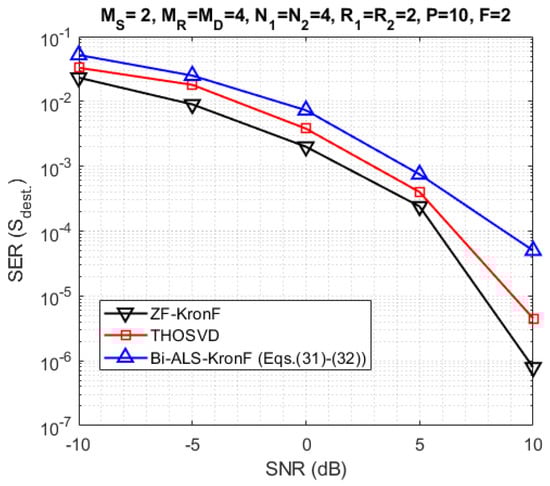
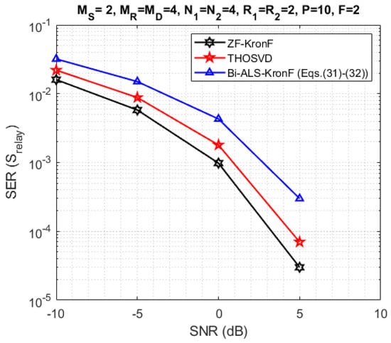
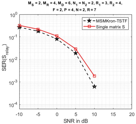
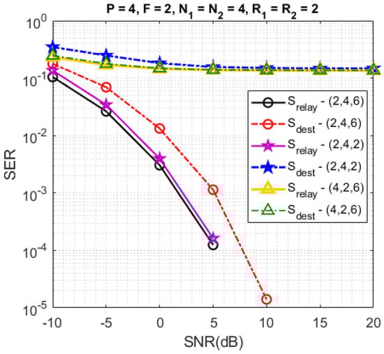
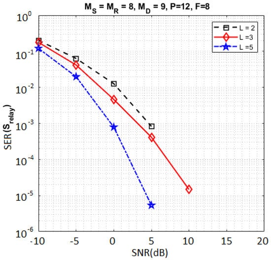
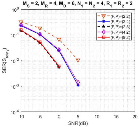
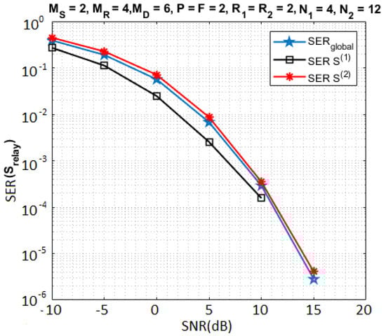
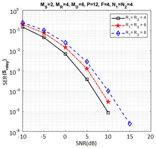
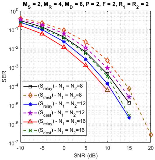
Table 6.
Parameters for the simulations.
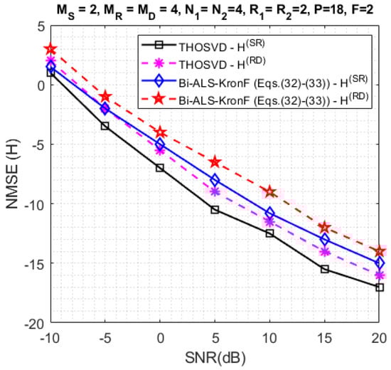
Figure 9.
Comparison of the TSTF-MSMKron and TSTF codings.
Figure 8.
Impact of different numbers of antennas.
Figure 7.
Impact of L on the SER.
Figure 6.
Impact of different configurations of .
Figure 5.
Impact on the SER of individual symbol matrices.
Figure 4.
Impact of data stream numbers.
Figure 3.
Impact of numbers of symbols per data stream.
Table 6.
Parameters for the simulations.
| Figures | Impact of | Parameters |
|---|---|---|
| Figure 3 | Number of symbols per data stream | ; ;; |
| ; | ||
| Figure 4 | Number of data streams | ; ; |
| ; ; | ||
| Figure 5 | Different configurations for and | ; ; |
| ; ; | ||
| Figure 6 | Different configurations for (F, P) | ; ; ; |
| (F, P) | ||
| Figure 7 | Number of symbol matrices | : ; ; ; |
| ; | ||
| : ; | ||
| ; ; ; ; | ||
| ; ; | ||
| : ; ; ; ; ; ; | ||
| Figure 8 | Different antenna configurations | ; ; ; ; |
| Figure 9 | Comparison of the TSTF-MSMKron and TSTF codings | ; ; ; |
| ; ; ; ; | ||
| Figure 10, Figure 11 and Figure 12 | Comparison of the proposed semi-blind receivers | ; ; |
| ; ; |
Table 7.
Transmission rate for different configurations.
Table 7.
Transmission rate for different configurations.
| Figures | Parameters | Transmission Rate (T) |
|---|---|---|
| Figure 3 | T = 0.468; 0.319; 0.242 | |
| Figure 4 | T = 0.156; 0.239; 0.322 | |
| Figure 5 | ; | T = 0.625 |
| Figure 6 | T = 0.875; 0.437; 0.218; 0.437; 0.218 | |
| Figure 7 | T = 0.0781 | |
| Figure 8 | T = 0.437 | |
| Figure 9 | Comparison of the TSTF-MSMKron and TSTF codings | T = 1.5; = 7 |
| Figure 10, Figure 11 and Figure 12 | Comparison of the proposed semi-blind receivers | T = 0.094 |
Figure 3 shows the impact on the SER for different numbers of symbols per data stream: , where and denote the SER at the relay and the destination, respectively. From these simulation results, it can be concluded that the SER is improved when the numbers of symbols increase, which implies an increase of coding diversity, since is a dimension of the contracted form and of the data tensors, which is not the case for . On the other hand, the transmission rate decreases as shown in Table 7. In addition, note that the SER at the relay is better than the one at the destination. This happens because with the DF protocol, the symbols are estimated and decoded before they are retransmitted by the relay to the destination, which induces a propagation error due to the decoding.
Figure 4, Figure 5, Figure 6, Figure 7, Figure 8 and Figure 9 present the SER obtained at the relay (). Figure 4 compares the SER for three different data stream numbers: . From this figure, it can be concluded that increasing and implies an increase of the number of symbols to be estimated without increasing the number of data in the tensor for performing the symbol estimation, thus inducing a degradation of the SER, while the transmission rate increases (see Table 7).
In Figure 5, the simulation results compare the SERglobal with the individual SERs for and when , and . For this configuration, the Kronecker product between and induces a greater diversity for than for due to the fact that each symbol of is repeated times while each symbol of is repeated only times. That implies an SER smaller for than for .
Figure 6 presents the results considering different configurations for the numbers of subcarriers (F) and time blocks (P). Note that a performance improvement is obtained when F and/or P are/is increased due to an increase of frequency and/or time diversities. On the other hand, the transmission rate decreases. We can also remark that for the same value of the product or , the diversity gain is the same, implying very close SERs, which illustrates the symmetric role played by the frequency and time diversities in the SER performance.
In Figure 7, we compare the SER for different numbers of symbol matrices . The design parameters have been chosen so that the transmission rate is the same for the three values of L. The MSMKron scheme with provides the best SER performance in comparison with . These results corroborate the coding gain provided by the Kronecker product of symbol matrices.
In Figure 8, the SERs are plotted for different configurations of antenna numbers . Comparing these configurations, we note that the best SER is obtained when . For the configuration , the SER is not good both at the relay and the destination, because the identifiability condition () at the relay is not satisfied. For the configuration , the SER at the relay is similar to the one for the configuration because the antenna numbers are the same for both configurations, but the SER at the destination is not good because the identifiability condition () at the destination is not satisfied for the configuration , which is not the case of the configuration . With this last configuration, we note that the SER at the relay is better than the one at the destination.
In Figure 9, the proposed TSTF-MSMKron coding is compared with the TSTF coding, i.e., using a single symbol matrix instead of a multiple Kronecker product of symbol matrices. With the TSTF coding, the symbol matrix is estimated using Equation (31), and the transmission rate is given by:
For both codings, the number (14) of transmitted symbols is the same. See the design parameters in Table 6.
As expected, from Figure 9, we conclude that the TSTF-MSMKron coding gives a better SER than the TSTF coding thanks to a greater coding diversity brought by the Kronecker product of symbol matrices. As a counterpart, the transmission rate with the TSTF-MSMKron coding is smaller than the one with the TSTF coding. See Table 7.
6.3. Comparison of THOSVD and Bi-ALS-KronF Receivers
In the next experiments, we compare the SERs obtained with the proposed semi-blind and ZF-KronF receivers. First, the results are presented in terms of SER at the relay (-Figure 10) and the destination (-Figure 11). Then, we compare the performance of semi-blind receivers in terms of channel NMSE at each hop (Figure 12). For these simulations, the design parameters are fixed with the following values: , , , , , and .
From Figure 10 and Figure 11, we can conclude that the THOSVD receiver provides a better SER performance than the Bi-ALS-KronF receiver. That is due to the closed form of the THOSVD receiver allowing to jointly estimate the channel and symbol matrices, while the Bi-ALS-KronF receiver is composed of two steps, one iterative and one closed form. On the other hand, the THOSVD receiver is more constraining in terms of identifiability conditions () than the Bi-ALS-KronF receiver, inducing a reduction of the transmission rate, as can be seen in Table 7. It can also be noted that the SER at the relay is better than the one at destination due to the error propagation caused by decoding at the relay. As expected, the ZF-KronF receiver provides the best SER due to an a priori knowledge of the channels.
In Figure 12, the channel NMSE results obtained at each hop are plotted. Note that the THOSVD receiver gives better results than the Bi-ALS-KronF one. As for the SER, this is because the THOSVD is a closed-form solution, while the Bi-ALS algorithm is iterative. Moreover, the channel estimation in the first hop is slightly better than the one in the second hop. This is due to error propagation in the re-transmission of symbol matrices after decoding at the relay.
Note that considering non-coherent receivers [36,37,38] would imply avoiding the assumption about the knowledge of the coding tensors and used at the source and the relay, which would require a fully blind approach. Such a non-coherent assumption would destroy the essential uniqueness property of the estimated channels and symbols (up to scaling ambiguities). More specifically, in the non-coherent case, the Tucker models defined in Equations (15) and (26) would be affected by rotational ambiguities, which means that the channel tensors and symbol matrices estimated at the relay and destination nodes would be linked to the true ones via a transformation by a nonsingular matrix. It should be mentioned that one possible way to ensure the successful decoding of transmitted symbols in the non-coherent case, where such rotational ambiguities are present, is to consider Grassmannian constellations for symbol matrices, as proposed in [39,40].
7. Conclusions
In this paper, we have proposed a new two-hop CDMA-OFDM MIMO system which combines a tensor space–time–frequency (TSTF) coding with a multiple Kronecker product of symbol matrices, leading to the so-called TSTF-MSMKron coding. This new coding makes it possible to improve the gains in diversity and throughput. We have shown that the tensors of signals received at the relay and destination nodes satisfy two generalized Tucker models whose core tensors are the coding tensors.
Assuming these coding tensors are known, two semi-blind receivers have been derived to jointly estimate the transmitted information symbols and the channels. One, called the Bi-ALS-KronF receiver, is composed of two stages. In the first stage, the iterative ALS algorithm is used to estimate the channel and the Kronecker product of symbol matrices, while in the second stage, the KronF method is applied to separate the symbol matrices. The other one, called THOSVD receiver, is a closed-form solution which allows simultaneously estimating the channel and the symbol matrices by means of SVD computations as with the KronF method. Necessary conditions for system identifiability have been established for each receiver, showing that the THOSVD receiver is more constraining than the Bi-ALS-KronF one for the choice of the number of time blocks and consequently from the data rate point of view.
It is worth mentioning that the proposed two-hop system can be easily extended to the multi-hop case owing to the use of the DF protocol at the relay, since the tensor models for the signals received at the relays and destination have the same structure (generalized Tucker models), with the correspondences (23) and (24) established between the first and second hops. These correspondences can be easily generalized to more than two hops if the same coding scheme is used at each relay.
Extensive Monte Carlo simulations have allowed illustrating the impact of all the design parameters on the SER performance using the ZF receiver. In particular, the diversity gain brought by each parameter of the TSTF-MSMKron coding has been analyzed. The performances of the proposed semi-blind receivers have been compared in terms of SER and channel NMSE. As expected, the THOSVD closed-form receiver outperforms the iterative Bi-Als-KronF receiver. Moreover, a comparison with the standard TSTF coding has corroborated the SER improvement brought by the MSMKron coding, which allows increasing the diversity gain.
Note that we have numerically evaluated the SER performance under different schemes, assuming 16-QAM constellation for all the symbol matrices involved in our MSMKron coding scheme. At this point, we do not have a theoretical SER performance evaluation. Deriving an analytical Cramer–Rao bound (CRB) for the estimated channels and symbols is challenging, and this constitutes an important perspective for this work.
Among some other perspectives of this work, we can mention an extension of the proposed relaying system to the multi-hop case using the amplify-and-forward (AF) protocol and taking resource allocation tensors into account. Such considerations will lead to new tensor models and therefore new semi-blind receivers. Other extensions concern the development of relaying systems with TSTF-MSMKron coding for double-directional dual-polarized MIMO systems and intelligent reflecting surfaces (IRS)-assisted systems.
Author Contributions
Conceptualization and methodology: G.F.; Software and simulations: P.H.U.d.P. and M.d.F.K.B.C.; Original writing of the manuscript: P.H.U.d.P. and M.d.F.K.B.C.; Review of the writing: G.F., A.L.F.d.A. and J.P.J.d.C.; Research supervision and editing: G.F. All authors have read and agreed to the published version of the manuscript.
Funding
This research was funded by the Federal District Research Foundation (Fundação de Apoio à Pesquisa do Distrito Federal—FAP/DF), Brazil.
Institutional Review Board Statement
Not applicable.
Informed Consent Statement
Not applicable.
Data Availability Statement
Not applicable.
Acknowledgments
The authors thank the support of the Coordination for the Improvement of Higher Education Personnel (CAPES), the Brazilian National Council for Scientific and Technological Development (CNPq) [303343/2017-6], University of Brasília (UnB) and IT Doctoral School (ED STIC) of the Université Côte d’Azur.
Conflicts of Interest
The authors declare having no conflict of interest.
Abbreviations
The following abbreviations are used in this manuscript:
| 4G | fourth-generation |
| 5G | fifth-generation |
| 6G | sixth-generation |
| AF | amplify-and-forward |
| ALS | alternating least squares |
| Bi-ALS | bi-alternating least squares |
| CDMA | code division multiplexing access |
| CSI | channel state information |
| DF | decode-forward |
| DFT | discrete Fourier transform |
| DKRF | double KRF |
| HONTD | high-order nested Tucker decomposition |
| IoT | internet of things |
| KRF | Khatri–Rao factorization |
| KRST | Khatri–Rao space-time |
| KRSTF | Khatri–Rao space-time-frequency |
| KronF | Kronecker factorization |
| LM | Levenbergh–Marquardt |
| LS | least squares |
| LSKP | LS estimation of Kronecker products |
| MIMO | multiple input multiple output |
| MKRF | multiple Khatri–Rao factorization |
| MKRSM | multiple Khatri–Rao product of symbol matrices |
| MKRST | multiple Khatri–Rao space–time |
| MKronST | multiple Kronecker space–time |
| MSMKron | multiple symbol matrices Kronecker product |
| NMSE | normalized mean square error |
| OFDM | orthogonal frequency division multiplexing |
| PARAFAC | parallel factors analysis |
| QAM | quadrature amplitude modulation |
| PSK | phase-shift keying |
| SER | symbol error rate |
| SNR | signal-to-noise ratio |
| ST | space–time |
| SVD | signal value decomposition |
| TD | Tucker decomposition |
| THOSVD | truncated higher-order singular value decomposition |
| TSTF | tensor space–time frequency |
| ZF | zero-forcing |
Appendix A. Kronecker Factorization (KronF) Algorithm
In this section, the KronF algorithm is presented for estimating the matrix factors of a multiple Kronecker product , with , for , by minimizing the LS cost function:
Following the idea introduced in [41] for a Kronecker product of two matrices, the problem is solved by rewriting the cost function (A1) in terms of approximation of a rank-one tensor built as the outer product of vectorized forms of the matrix factors, as:
where , and is the rank-one tensor obtained by reshaping the multiple Kronecker product:
Each vector is estimated using the THOSVD algorithm, and the matrix factor estimate is deduced using the unvec operator [29,32,42], with a scalar ambiguity which can be eliminated assuming the knowledge of one element of , e.g., , which leads to the following corrected estimate:
References
- Goldsmith, A. Wireless Communications; Cambridge University Press: Cambridge, UK, 2005. [Google Scholar]
- Chataut, R.; Akl, R. Massive MIMO systems for 5G and beyond networks—Overview, recent trends, challenges, and future research direction. Sensors 2020, 20, 2753. [Google Scholar] [CrossRef]
- Noohani, M.Z.; Magsi, K.U. A review of 5G technology: Architecture, security and wide applications. Int. Res. J. Eng. Technol. (IRJET) 2020, 7, 3440–3471. [Google Scholar]
- Sendonaris, A.; Erkip, E.; Aazhang, B. User cooperation diversity, Part I, System Description. IEEE Trans. Commun. 2003, 51, 1927–1938. [Google Scholar] [CrossRef]
- da Costa, M.N.; Favier, G.; Romano, J.M.T. Tensor modeling of MIMO communication systems with performance analysis and Kronecker receivers. Signal Process. 2018, 145, 304–316. [Google Scholar] [CrossRef]
- Venugopal, A.; Leib, H. A tensor based framework for multi-domain communication systems. IEEE Open J. Commun. Soc. 2020, 1, 606–633. [Google Scholar] [CrossRef]
- Tucker, L.R. Some mathematical notes on three-mode factor analysis. Psychometrika 1966, 31, 279–311. [Google Scholar] [CrossRef]
- Harshman, R.A. Foundations of the PARAFAC procedure: Models and conditions for an “explanatory” multimodal factor analysis. UCLA Work. Pap. Phon. 1970, 16, 1–84. [Google Scholar]
- Du, J.; Han, M.; Jin, L.; Hua, Y.; Li, X. Semi-blind receivers for multi-user massive MIMO relay systems based on block Tucker2-PARAFAC tensor model. IEEE Access 2020, 8, 32170–32186. [Google Scholar] [CrossRef]
- Wang, Z.; Cai, Y.; Liu, A.; Wang, J.; Yue, G. Mixed-timescale channel estimation for MIMO relay multi-user systems based on the PARAFAC decomposition. IEEE Commun. Lett. 2021, 25, 1288–1292. [Google Scholar] [CrossRef]
- Zilli, G.M.; Zhu, W.P. Constrained tensor decomposition-based hybrid beamforming for mmWave massive MIMO-OFDM communication systems. IEEE Trans. Veh. Technol. 2021, 70, 5775–5788. [Google Scholar] [CrossRef]
- Han, X.; Zhou, Y.; de Almeida, A.L.F.; Freitas, W.D.C. Semi-blind Uni-ALS receiver for a two-way MIMO relaying system based on the PARATUCK2 model. Digit. Signal Process. 2021, 110, 102916. [Google Scholar] [CrossRef]
- Du, J.; Han, M.; Chen, Y.; Jin, L.; Gao, F. Tensor-based joint channel estimation and symbol detection for time-varying mmWave massive MIMO systems. IEEE Trans. Signal Process. 2021, 69, 6251–6266. [Google Scholar] [CrossRef]
- Du, J.; Ye, S.; Jin, L.; Li, X.; Ngo, H.Q.; Dobre, O.A. Tensor-Based Joint Channel Estimation for Multi-Way Massive MIMO Hybrid Relay Systems. IEEE Trans. Veh. Technol. 2022, 71, 9571–9585. [Google Scholar] [CrossRef]
- de Almeida, A.L.F.; Favier, G. Double Khatri-Rao space-time-frequency coding using semi-blind PARAFAC based receiver. IEEE Signal Process. Lett. 2013, 20, 471–474. [Google Scholar] [CrossRef]
- Favier, G.; Fernandes, C.A.R.; de Almeida, A.L.F. Nested Tucker tensor decomposition with application to MIMO relay systems using tensor space–time coding (TSTC). Signal Process. 2016, 128, 318–331. [Google Scholar] [CrossRef]
- Randriambelonoro, S.V.N.; Favier, G.; Boyer, R. Semi-blind joint symbols and multipath parameters estimation of MIMO systems using KRST/MKRSM coding. Digit. Signal Process. 2021, 109, 102908. [Google Scholar] [CrossRef]
- Ximenes, L.; Favier, G.; de Almeida, A.L.F. Semi-blind receivers for non-regenerative cooperative MIMO communications based on nested PARAFAC modeling. IEEE Trans. Signal Process. 2015, 63, 4985–4998. [Google Scholar] [CrossRef]
- Ximenes, L.; Favier, G.; de Almeida, A.L.F. Closed-form semi-blind receiver for MIMO relay systems using double Khatri-Rao space-time coding. IEEE Signal Process. Lett. 2016, 23, 316–320. [Google Scholar] [CrossRef]
- Rocha, D.S. Nested Tensor Decomposition Applied to Cooperative MIMO Communication Systems. Ph.D. Thesis, University of Ceará, Fortaleza, Brazil, 2019. [Google Scholar]
- Rocha, D.S.; Favier, G.; Fernandes, C.A.R. Closed-form receiver for multi-hop MIMO relay systems with tensor space-time coding. J. Commun. Inf. Syst. 2019, 34, 50–54. [Google Scholar] [CrossRef]
- Han, X.; Ying, J.; Liu, A.; Ma, L. A nested tensor-based receiver employing triple constellation precoding for three-hop cooperative communication systems. Digit. Signal Process. 2023, 133, 103862. [Google Scholar] [CrossRef]
- Wang, Z.; Cai, Y.; Liu, A.; Wang, J.; Yue, G. Two-timescale uplink channel estimation for dual-hop MIMO relay multi-user systems. IEEE Trans. Veh. Technol. 2021, 70, 4724–4739. [Google Scholar] [CrossRef]
- Ximenes, L.; Favier, G.; de Almeida, A.L.F.; Silva, Y.C.B. PARAFAC-PARATUCK semi-blind receivers for two-hop cooperative MIMO relay systems. IEEE Trans. Signal Process. 2014, 62, 3604–3615. [Google Scholar] [CrossRef]
- Freitas, W.d.C.; Favier, G.; de Almeida, A.L.F. Sequential closed-form semi-blind receiver for space-time coded multi-hop relaying systems. IEEE Signal Process. Lett. 2017, 24, 1773–1777. [Google Scholar] [CrossRef]
- Freitas, W.d.C.; Favier, G.; de Almeida, A.L.F. Generalized Khatri-Rao and Kronecker space-time coding for MIMO relay systems with closed-form semi-blind receivers. Signal Process. 2018, 151, 19–31. [Google Scholar] [CrossRef]
- Favier, G.; da Costa, M.N.; de Almeida, A.L.F.; Romano, J.M.T. Tensor space-time (TST) coding for MIMO wireless communication systems. Signal Process. 2012, 92, 1079–1092. [Google Scholar] [CrossRef]
- Rocha, D.S.; Fernandes, C.A.R.; Favier, G. MIMO multi-relay systems with tensor space-time coding based on coupled nested Tucker decomposition. Digit. Signal Process. 2019, 89, 170–185. [Google Scholar] [CrossRef]
- Sokal, B.; de Almeida, A.L.F.; Haardt, M. Semi-blind receivers for MIMO multi-relaying systems via rank-one tensor approximations. Signal Process. 2020, 166, 107254. [Google Scholar] [CrossRef]
- Favier, G.; de Almeida, A.L.F. Tensor space-time-frequency coding with semi-blind receivers for MIMO wireless communication systems. IEEE Trans. Signal Process. 2014, 62, 5987–6002. [Google Scholar] [CrossRef]
- de Lathauwer, L.; de Moor, B.; Vandewalle, J. A multilinear singular value decomposition. SIAM J. Matrix Anal. Appl. 2000, 21, 1253–1278. [Google Scholar] [CrossRef]
- Favier, G. Matrix and Tensor Decompositions in Signal Processing; Wiley: Hoboken, NJ, USA, 2021; Volume 2. [Google Scholar]
- Favier, G.; de Almeida, A.L.F. Overview of constrained PARAFAC models. EURASIP J. Adv. Signal Process. 2014, 2014, 142. [Google Scholar] [CrossRef]
- Jin, C.; Shevchenko, N.A.; Li, Z.; Popoy, S.; Chen, I.; Xu, T. Nonlinear coherent optical systems in the presence of equalization enhanced phase noise. J. Light. Technol. 2021, 14, 4646–4653. [Google Scholar] [CrossRef]
- Djordjevic, I.B. Spread Spectrum, CDMA, and Ultra-Wideband Communications. In Advanced Optical and Wireless Communications Systems; Springer International Publishing: Cham, Switzerland, 2022; pp. 647–712. [Google Scholar]
- Ngo, K.H.; Yang, S.; Guillaud, M.; Decurninge, A. Joint constellation design for the two-user non-coherent multiple-access channel. arXiv 2020, arXiv:2001.04970. [Google Scholar]
- Baeza, V.M.; Armada, A.G. User Grouping for Non-Coherent DPSK Massive SIMO with Heterogeneous Propagation Conditions. In Proceedings of the IEEE Global Congress on Electrical Engineering (GC-ElecEng), Valencia, Spain, 10–12 December 2021; pp. 260–330. [Google Scholar]
- Gohary, R.H.; Yanikomeroglu, H. Noncoherent MIMO signaling for block-fading channels: Approaches and challenges. IEEE Veh. Technol. Mag. 2019, 14, 80–88. [Google Scholar] [CrossRef]
- Decurninge, A.; Land, I.; Guillaud, M. Tensor-based modulation for unsourced massive random access. IEEE Wirel. Commun. Lett. 2020, 10, 552–556. [Google Scholar] [CrossRef]
- Luan, Z.; Wu, Y.; Liang, S.; Han, W.; Bai, B.; Zhang, L. Modulation for Massive Unsourced Random Access Based on Tensor Block Term Decomposition. In Proceedings of the IEEE Globecom Workshops (GC Wkshps), Rio de Janeiro, Brazil, 4–8 December 2022; pp. 637–643. [Google Scholar]
- Van Loan, C.F.; Pitsianis, N. Approximation with Kronecker products. In Linear Algebra for Large Scale and Real-Time Applications; Moonen, M.S., Golub, G.H., de Moor, B.L., Eds.; Kluwer Academic Publishers: Dordrecht, The Netherlands, 1993. [Google Scholar]
- Wu, K.K.; Yam, Y.; Meng, H.; Meshabi, M. Kronecker product approximation with multiple factor matrices via the tensor product algorithm. In Proceedings of the 2016 IEEE International Conference on Systems, Man and Cybernetics (SMC), Budapest, Hungary, 9–12 October 2016; pp. 4277–4282. [Google Scholar]
Disclaimer/Publisher’s Note: The statements, opinions and data contained in all publications are solely those of the individual author(s) and contributor(s) and not of MDPI and/or the editor(s). MDPI and/or the editor(s) disclaim responsibility for any injury to people or property resulting from any ideas, methods, instructions or products referred to in the content. |
© 2023 by the authors. Licensee MDPI, Basel, Switzerland. This article is an open access article distributed under the terms and conditions of the Creative Commons Attribution (CC BY) license (https://creativecommons.org/licenses/by/4.0/).