
Variable-Length Multiobjective Social Class Optimization for Trust-Aware Data Gathering in Wireless Sensor Networks


Abstract
1. Introduction
2. Literature Survey
2.1. Trust-Aware Data Gathering
2.2. MCDM for Data Gathering
3. Methodology
3.1. Definitions
3.1.1. Definition 1: Class
3.1.2. Definition 2: FAM
3.1.3. Definition 3: RAM
3.1.4. Definition 4: WCT
3.1.5. Definition 5: SCT
3.2. Overview of SC-MOPSO
| Algorithm 1 Pseudocode of SC-MOSPO for the V-length problem [42] |
| Input 1-NumOfParticles 2-NumOfIterations 3-Boundary 4-DimensionsRange 5-ObjectiveFunctions 6-Inertia,C1,C2 7-adaptiveTimeOut 8-classMinThreshold Output 1-ParetoFront 2-ParetoSet Start Algorithm 1: initSwarm(NumOfParticles) 2: numOfClass = DimensionsRange.Max − DimensionsRange.Min + 1; 3: for i = 1 until NumOfParticles 4: Dimension = genRan(DimensionsRange) 5: particle = genRan(Dimension,Boundary) 6: add particle to swarm 7: end 8: Classes = Distribute(swarm) 9: for iteration = 1 until NumOfIterations 10: for classIndex = 1 until length(Classes) 11: for each particle of Classes(classIndex) 12: exemplar = selectExemplar(Classes(classIndex)//-1- 13: newParticle = moveParticle(particle,exemplar,Inertia,C1,C2) 14: if(NoImprove(newParticle,particle)) 15: particle.counter = particle.counter + 1; 16: else 17: particle.counter = 0; 18: particle = newParticle; 19: end 20: end 21: end 22: for classIndex = 1 until length(Classes) 23: for each particle of Classes(classIndex) 24: adaptiveTimeOut = timeoutUpdate(particle.nonImpWindow, maxTimeOut) 25: if(particle.counter > adaptiveTimeOut and length(particle. Class) > classMinThreshold) 26: Class = selectNewClass(particle) 27: particle = moveToNewClass(particle, Class) 28: end 29: end 30: end 31: end 32: end End Algorithm |
3.3. SC-MOPSO-DG
3.3.1. Mathematical Model of Objective Space
- (1)
- Trust
- (2)
- Energy Consumption
- (3)
- Cost
- (4)
- Time
- (5)
- Noncoverage
3.3.2. Initialization
| Algorithm 2 Initialization of SC-MOPSO-DG |
| Inputs 1- 2- 3- 4- Output: 1- 2- 3- Start Algorithm 1: = struct() 2: ms = struct() 3: Nms= randi( ()) ())]) 4: class= Nms 5: dim = 0 6: for i = 1:Nms do 7: solution.ms(i).NRP = struct() 8: Nrv = randi([() ()]) 9: for j = 1:Nrv do 10: solution.ms(i).NRP(j).pos = [rand*( (XI) − (XI) − rand*( (YI) − (YI))] 11: solution.ms(i).NRP(j).nHops = randi([() ()]) 12: End for 13: dim = dim + Nrv*length of one RV information 14: class = strcat(num2str(class),num2str(Nrv)) 15: end for End Algorithm |
3.3.3. Addition and Deletion of Rendezvous Point
| Algorithm 3 Pseudocode of adding and removing rendezvous points |
| Input 1-class: class for moving to it. 2-exemplar: individual solution of new class. 3-oldSolution: the particle needed to moved. Output 1-newSolution Start Algorithm 1: newSolution = oldSolution 2: for each ms of newSolution do 3: difference = number of RV(ms) of exemplar − number of RV(ms) 4: if difference > 0 then 5: for i = 1 until difference do 6: select RVs randomly from exemplar 7: add them to ms newSolution 8: end for 9: else if difference < 0 then 10: for i = 1 until difference do 11: delete RV randomly 12: end for 13: end if 14: end for End Algorithm |
3.3.4. Moving to a Higher Class
| Algorithm 4 Move to higher class |
| Input 1-class: class for moving to it. 2-exemplar: individual solution of new class. 3-oldParticle: the particle needed to moved. 4-difference: difference between the number of mobile sinks of old and new class particle Output 1-newParticle. Start Algorithm 1: newParticle = oldParticle 2: for i = 1 until difference do 3: select random ms(exemplar) and add it to newParticle 4: end for 5: newParticle = AddDeleteRVs(newParticle, exemplar, class) End Algorithm |
3.3.5. Moving to a Lower Class
| Algorithm 5 Move to a lower class |
| Input 1-class: class for moving to it. 2-exemplar: individual solution of new class. 3-oldParticle: the particle needed to moved. 4-difference: difference between the number of mobile sinks of old and new class particle. Output 1-newParticle. Start Algorithm 1: newParticle = oldparticle 2: for i = 1 until difference) do 3: delete random ms from newParticle 4: end for 5: newParticle = AddDeleteRVs(exampler,newParticle,class) End Algorithm |
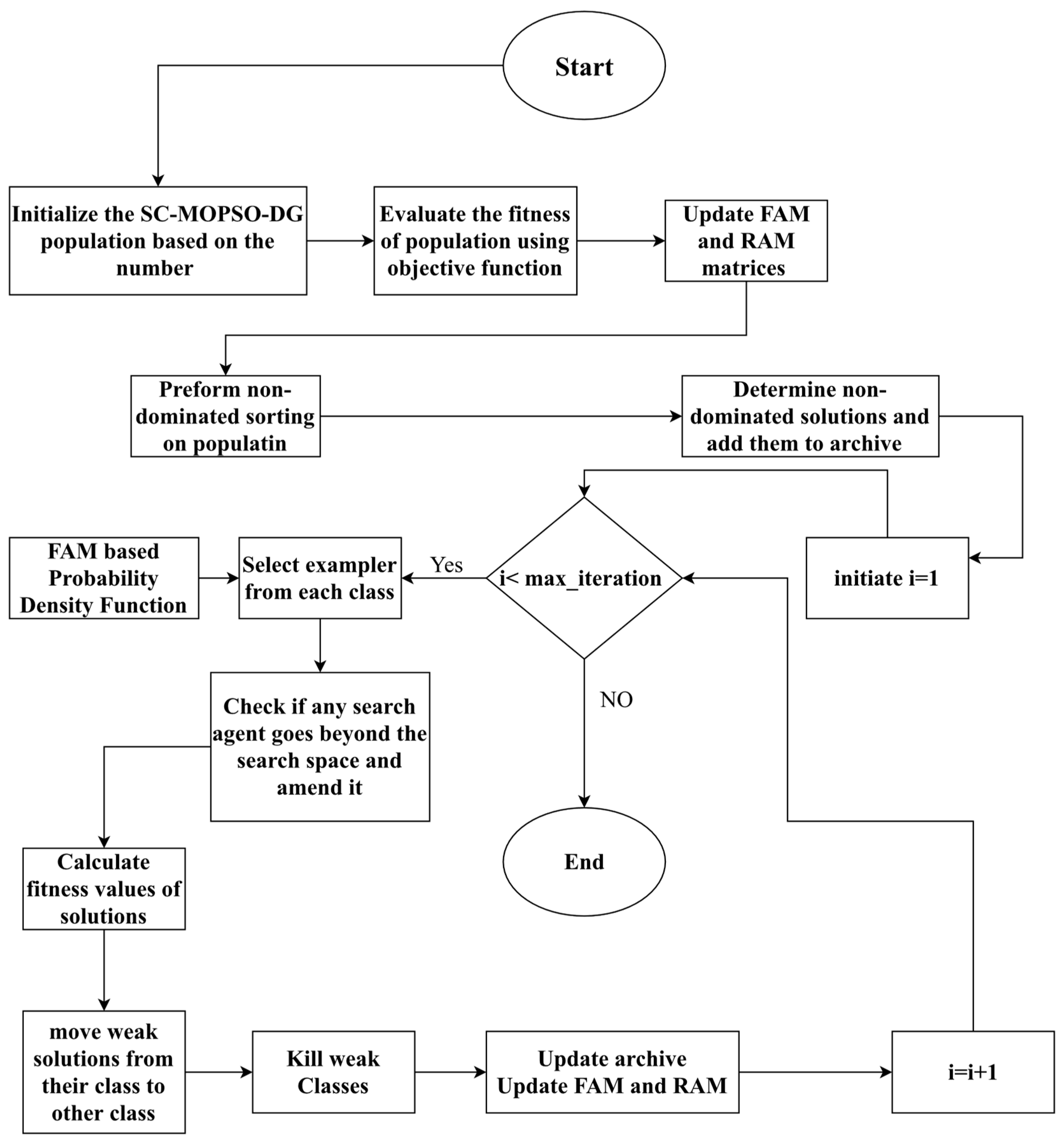
3.3.6. Main Algorithm
| Algorithm 6 Pseudocode of SC-MOPSO |
| Input 1- solution dimension 2- population size 3-max_iteration 4- … multi objective functions Output 1-Pareto front Start Algorithm 1: Initialize the SC-MOPSO-DG population based on the number 2: Evaluate the fitness of population using objective functions 3: It updates FAM and RAM matrices 4: Perform nondominated sorting on the population 5: Determine nondominated solutions and add them to archive using archive controller 6: For i = 1 until max_iteration 7: select exemplar from each class based on based probability density function 8: Update particle positions using algorithm Equations (1)–(4) and selected exemplars 9: Check if any search agent goes beyond the search space and amend it 10: Calculate fitness values of solutions, 11: update improvement counter for each solution 12: move weak solutions from their class to other class in case they are not improving 13: deletes weak class 14: call archive controller and update and RAM 15: Return archive End Algorithm |
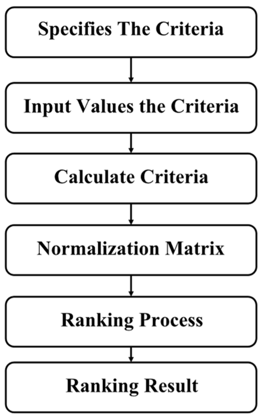
3.3.7. Simple Additive Weighting (SAW)
| Algorithm 7 Pseudocode of selecting solution from Pareto front using simple additive weight (SAW) |
| Input: paretoFront W objectives’ weights Output: objectivesOptFuncs Start: objectivesFuncs = paretoFront.solutionsObjectiveValues minValue = min(objectivesFuncs) maxValue = max(objectivesFuncs) normObjectives = (objectivesFuncs − minValue)/(maxValue − minValue) sumWObj = sum(normObjectives.*W) [minValues,index] = min(sumWObj) objectivesOptFuncs = paretoFront.solutionsObjectiveValues(index) End |
3.4. Example
3.5. Performance Metrics
4. Experiment and Results
4.1. MOO Evaluation
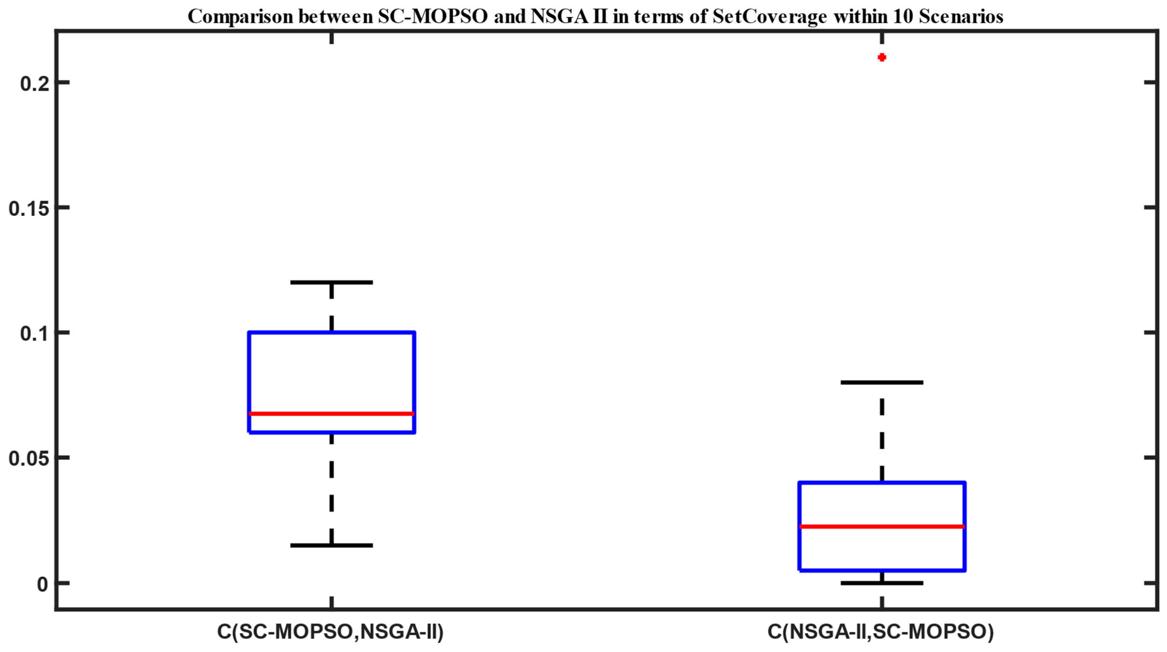
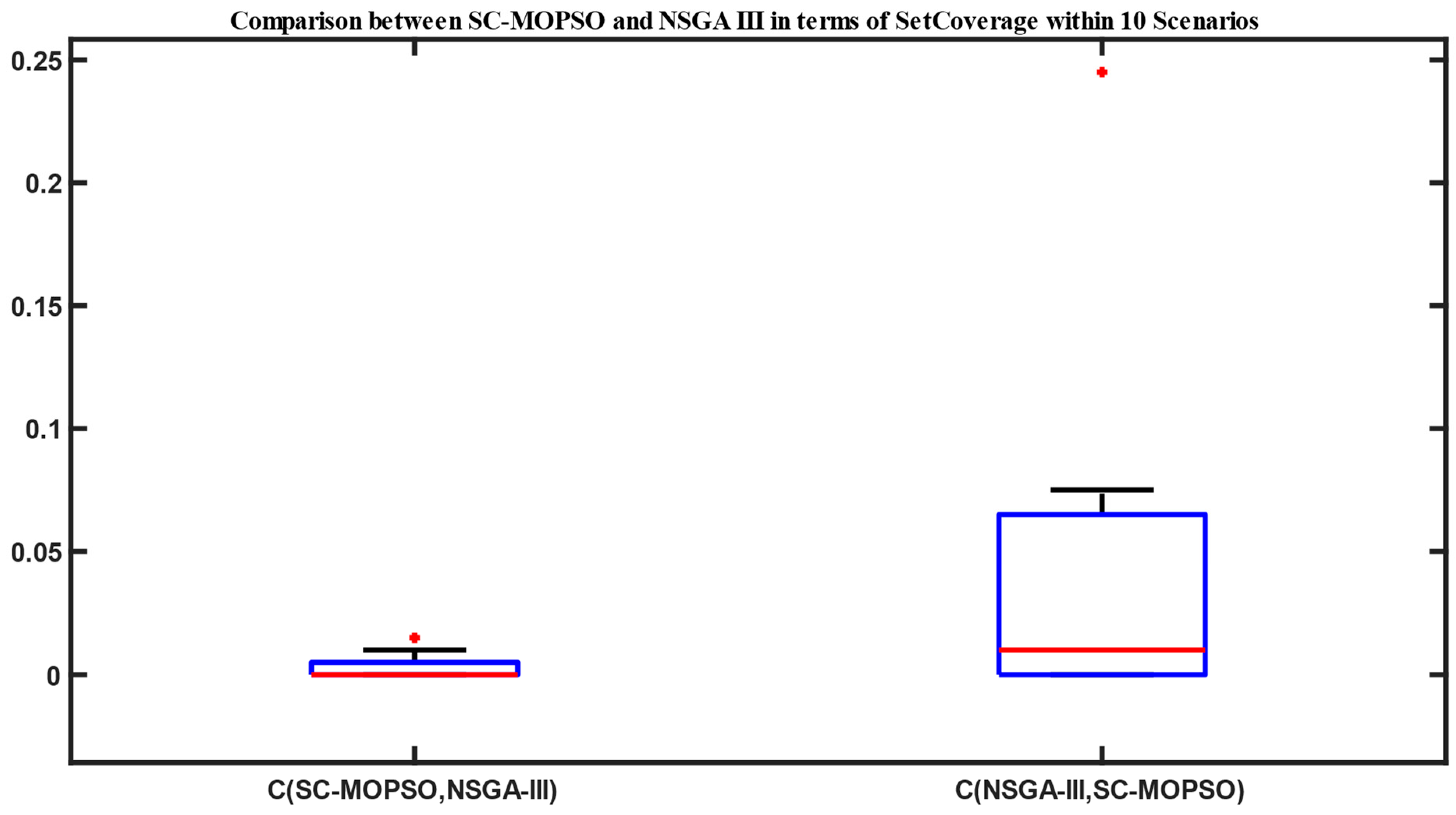
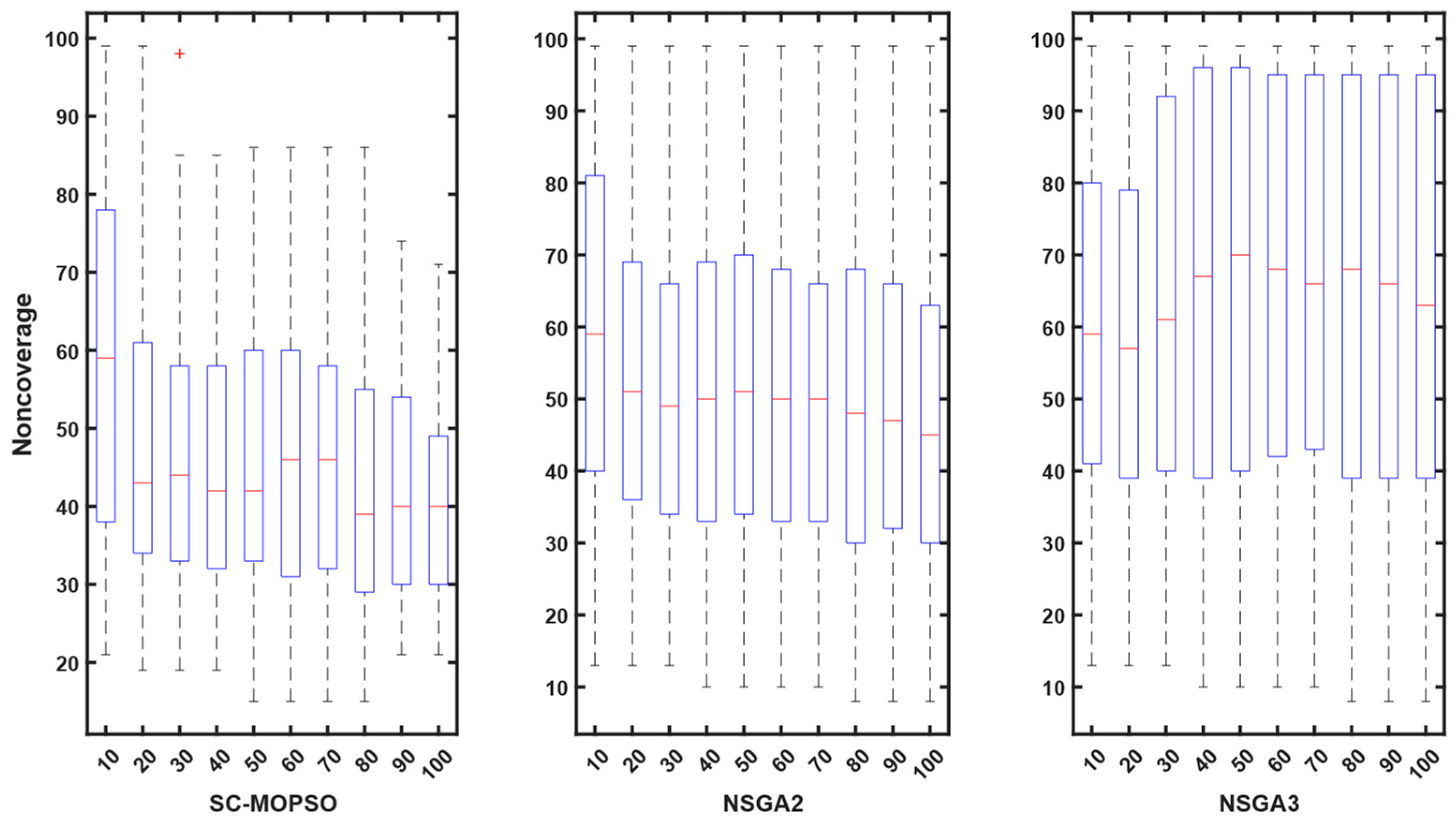
4.1.1. Set Coverage
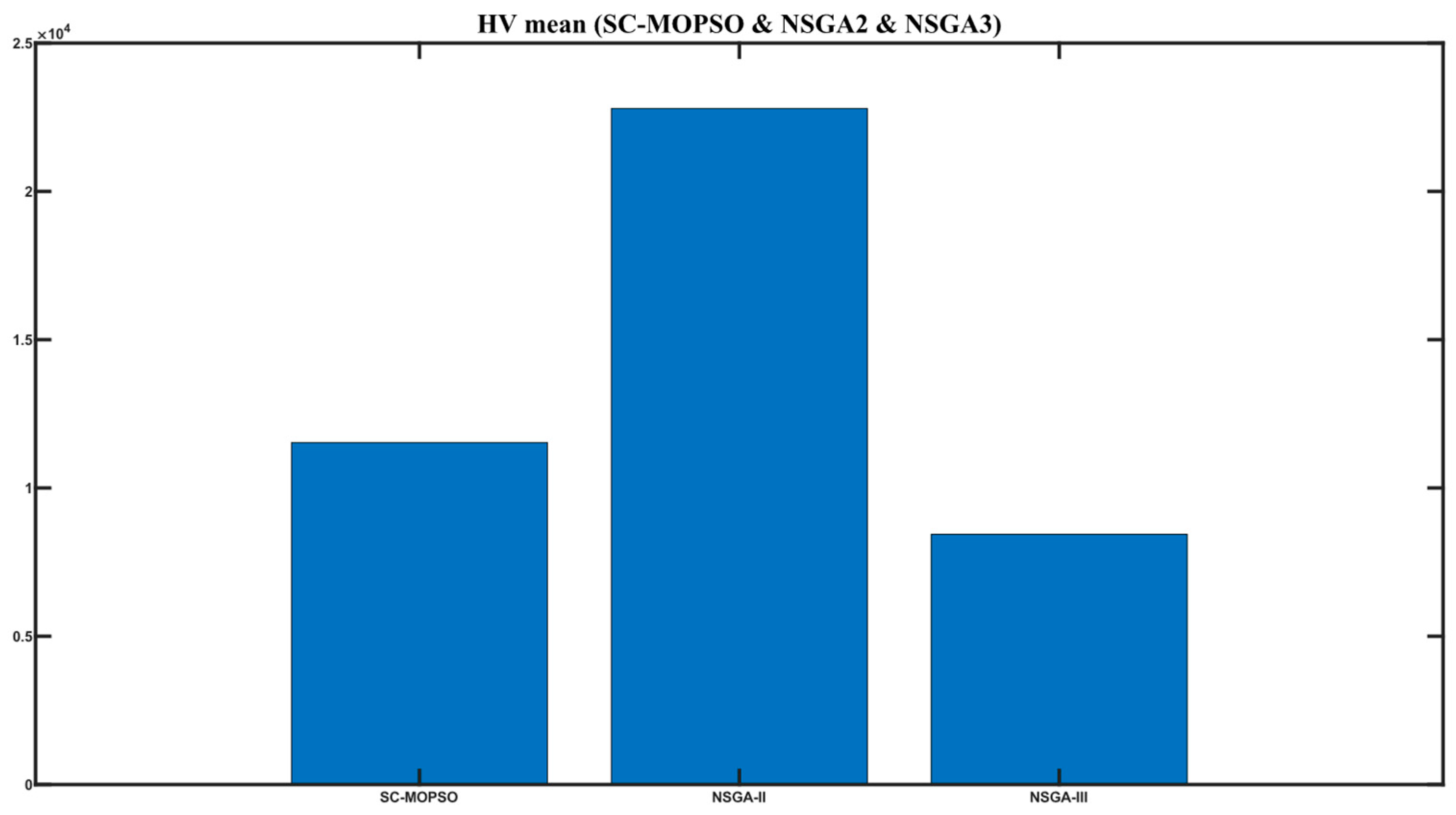
4.1.2. Hyper-Volume
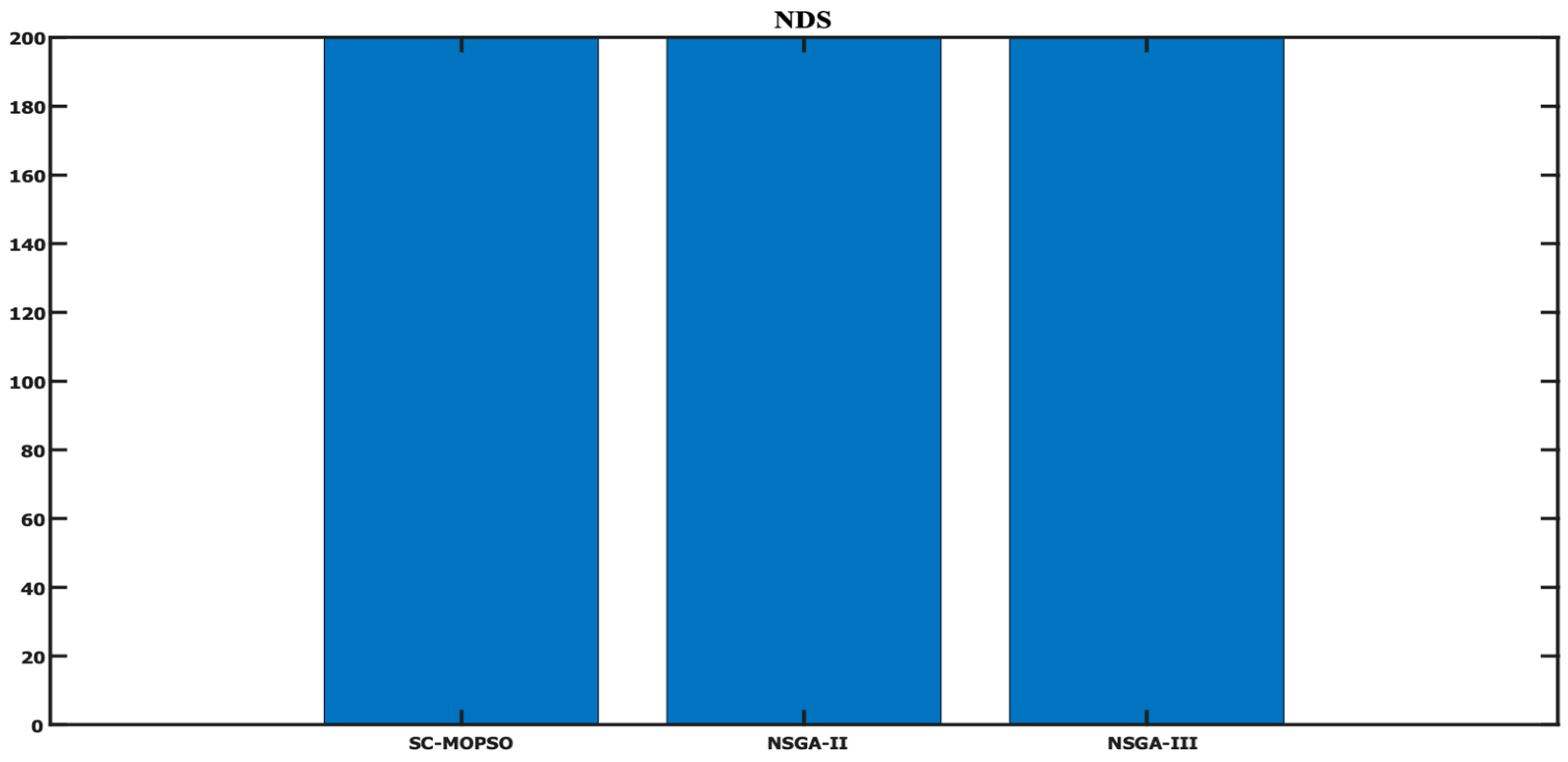
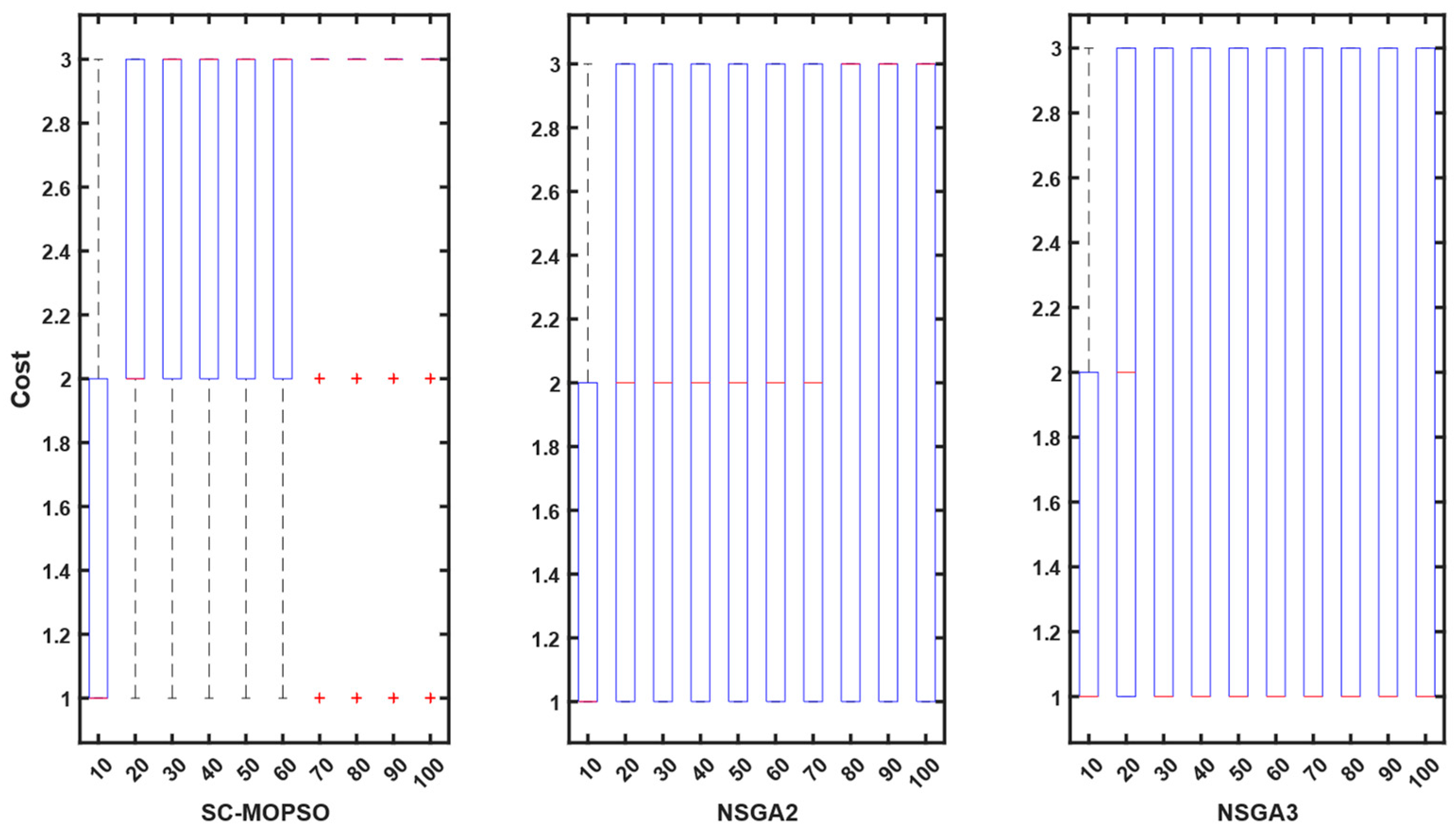
4.1.3. Number of Nondominated Solution
4.1.4. Convergence Graphs
4.2. Networking Measures
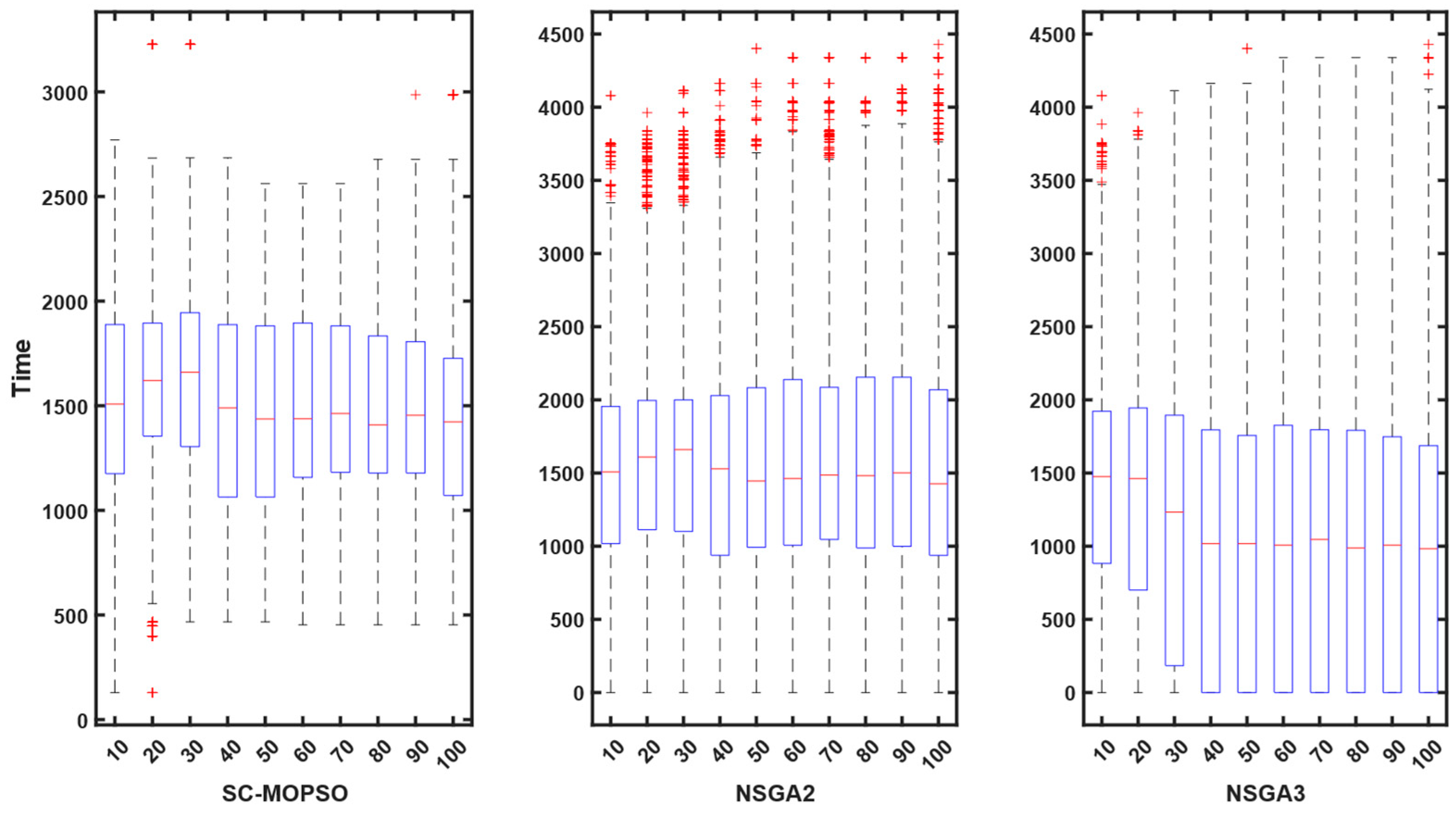
4.2.1. E2E Delay
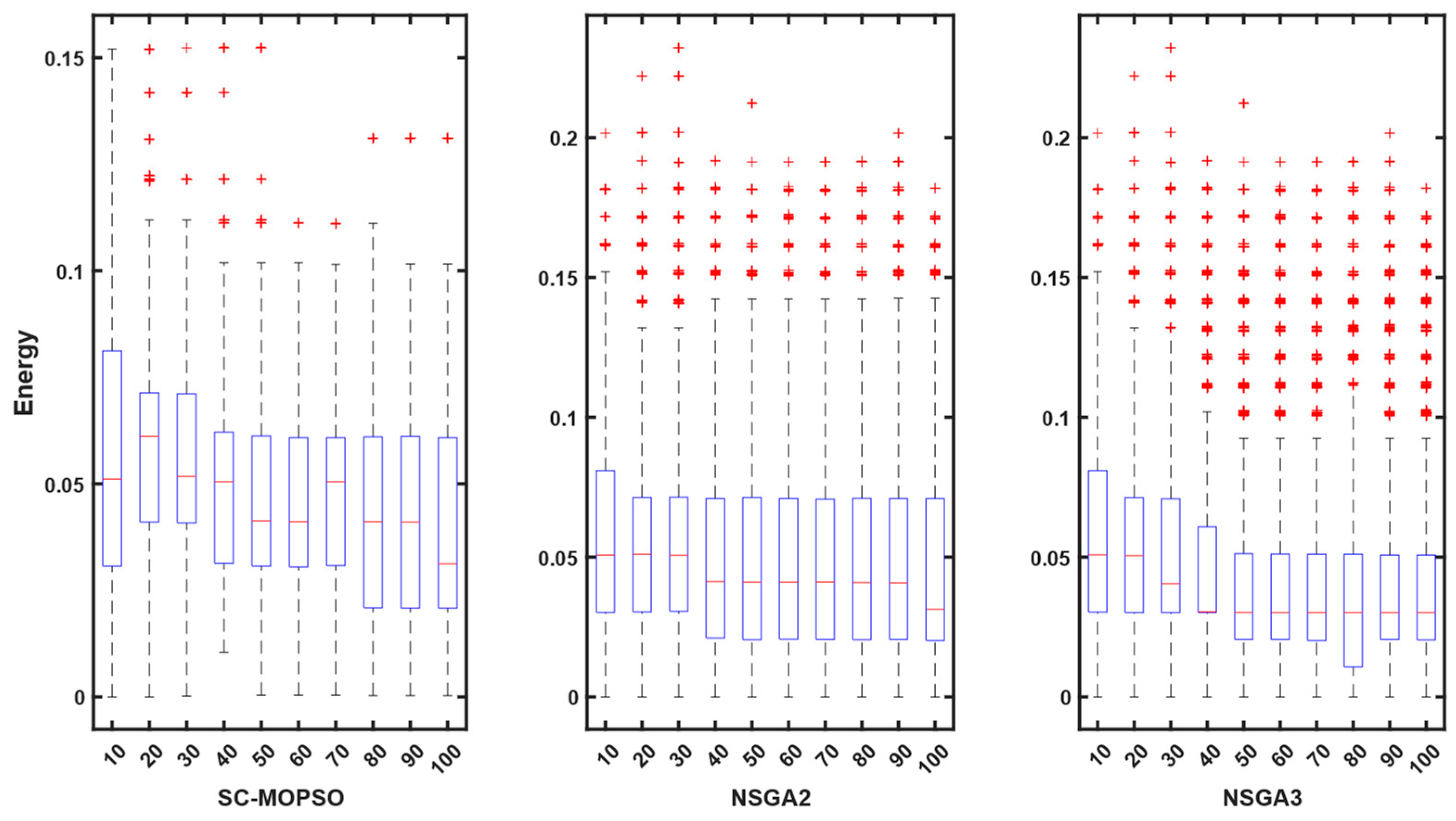
4.2.2. Energy Consumption
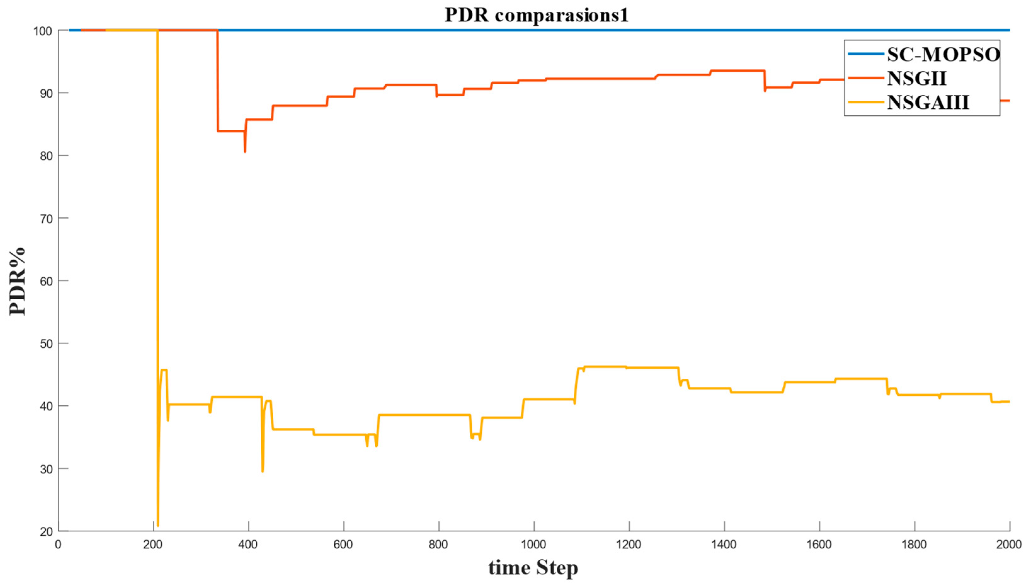
4.2.3. PDR
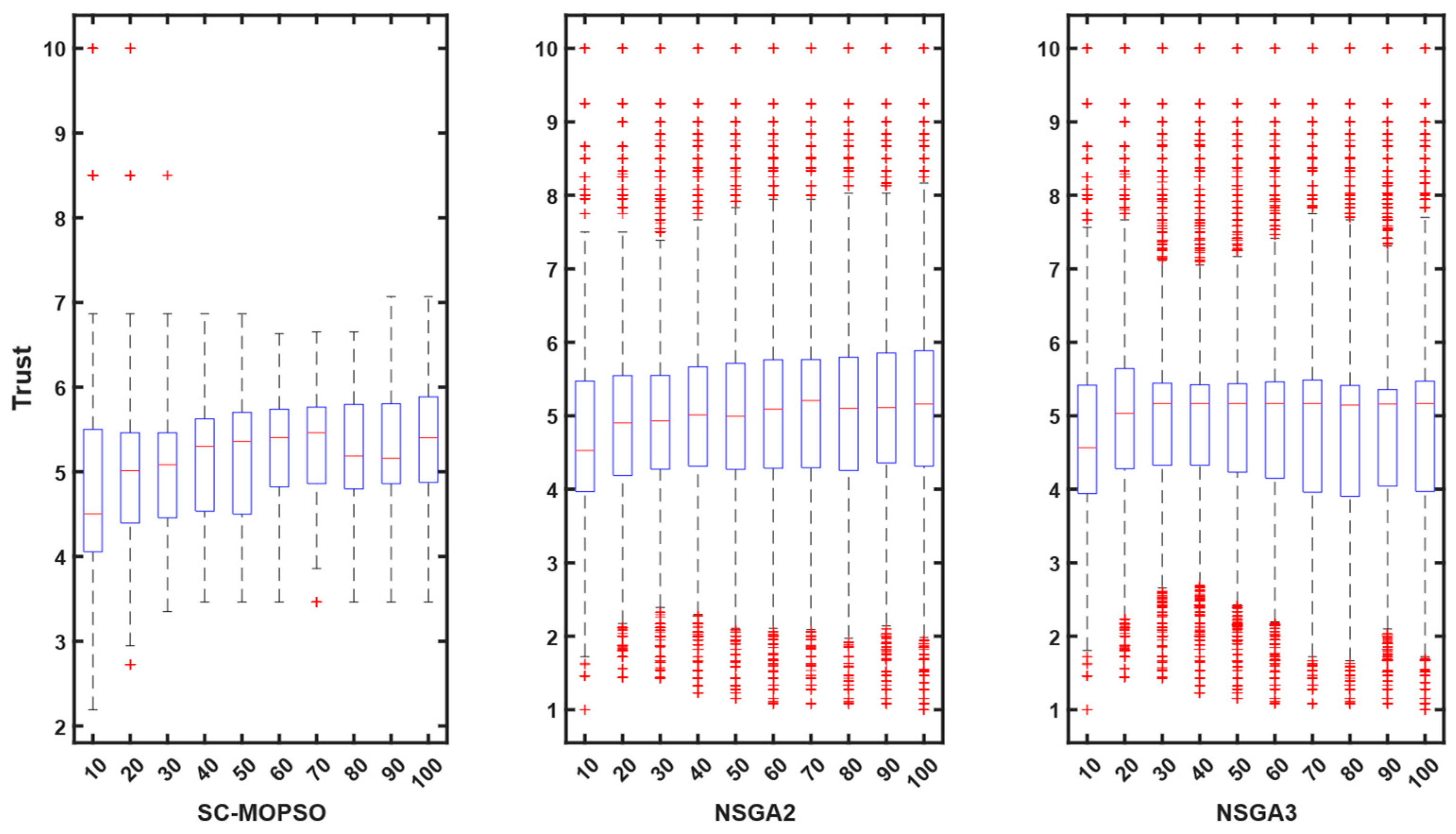
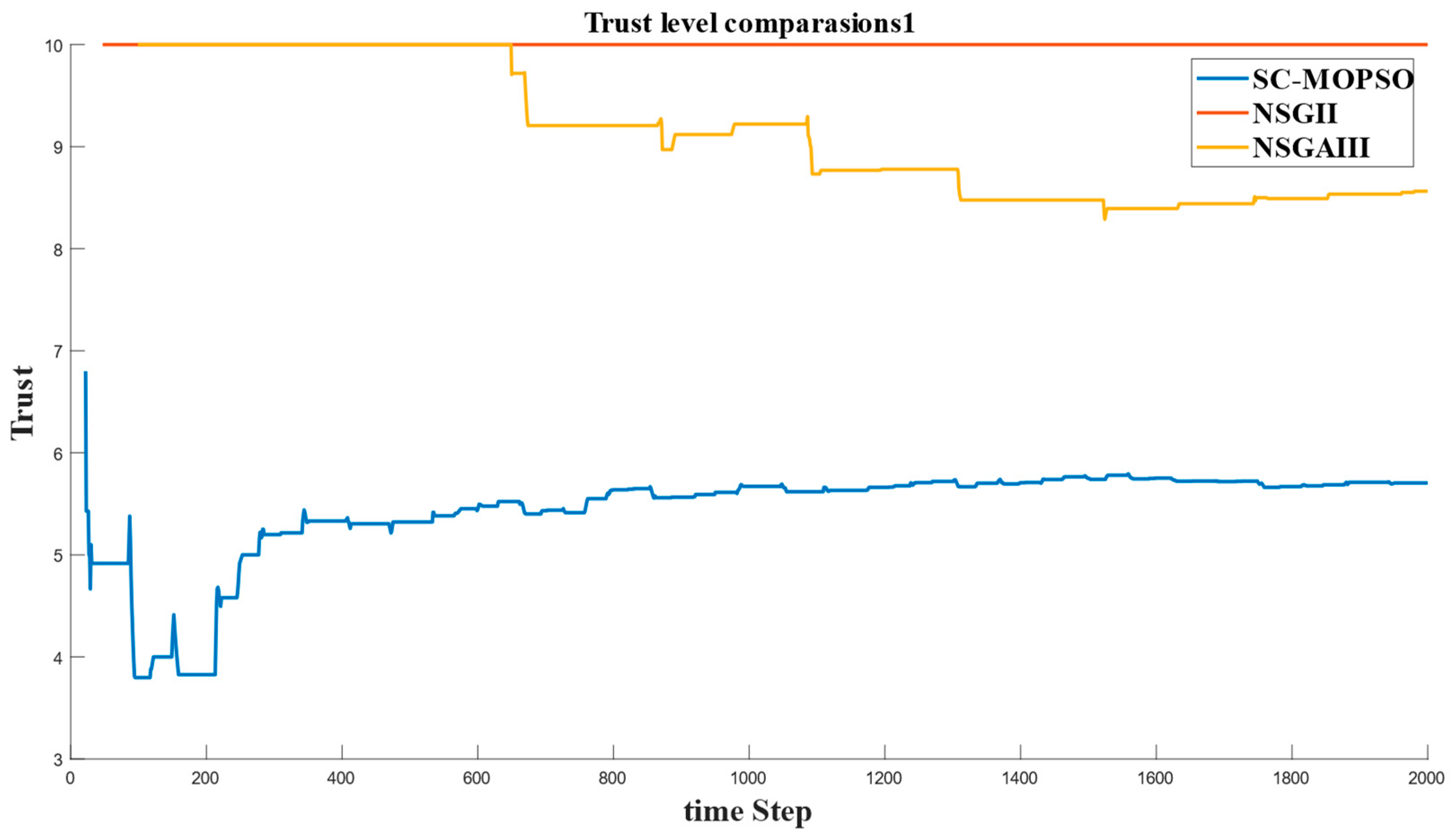
4.2.4. Trust
5. Discussion
6. Conclusions and Future Work
Author Contributions
Funding
Conflicts of Interest
Appendix A

| Article | Multiple Data Collector | Mobile Sensors | Dimension of Trustworthiness | Communication Trust | Distance between the Sensors | Packet Loss | Third-Party Recommendation | Energy | Number of Sensors | Area | Algorithms Used | Limitation | Simulation |
|---|---|---|---|---|---|---|---|---|---|---|---|---|---|
| [43] | Multiple dimensions | 100 | 300 × 300 | Virtual force-based modeling | Subject to local minima | MATLAB | |||||||
| [20] | Multiple dimensions | 250 | 100 × 100 | Probabilistic graph | Ignores various dimensions of trust | MATLAB | |||||||
| [24] | Two dimensions | 550 | 200 × 200 | secondary path optimization strategy | Ignores various dimensions of trust | MATLAB | |||||||
| [25] | Multiple dimensions | - | - | Temperature-Aware Trusted Routing Scheme (TTRS) | Sink is fixed | MATLAB | |||||||
| [21] | One dimension | 2000 | - | elliptic curve digital signature algorithm NSGA-II | It does not contain multi-dimension | MATLAB | |||||||
| [22] | One dimension | - | - | Energy-efficient mobile nodes-based algorithm using clustering | It does not contain a multi-dimension-based model for trust | NS3 | |||||||
| [26] | Two dimensions | 50 | 100 × 100 m | Believe based trust | Fixed single sink | OMNET ++ | |||||||
| [27] | Multiple dimensions | - | - | Aggregate Signature based Trust Routing | Fixed data aggregator | ||||||||
| [28] | Multiple dimensions | 54 | 100 × 100 | Trust-based data gathering | Stationary sink | MATLAB NS2 | |||||||
| [31] | Multiple dimensions | 30 | - | Trust Model based on the weighted average | Stationary sink | MATLAB | |||||||
| [29] | Multiple dimensions | 300 | 100 × 100 | Clustering | Stationary sink | MATLAB | |||||||
| [23] | Single dimension | 5 0 | 200 × 200 | Clustering | Stationary sink | - | |||||||
| [32] | Multiple dimensions | 50 | 100 × 100 | Dijkstra | Single mobile sink | MATLAB | |||||||
| [33] | Single dimension | - | Protocol | Fixed no Nodes | MATLAB | ||||||||
| [44] | Multiple dimensions | 1000 | 100 × 100 | Trust Model based on weighted average | It requires cloud management | MATLAB | |||||||
| OUR | Multiple dimensions | 100 | 200 × 200 | RL | Multiple mobile sink | MATLAB |
References
- Kirmani, S.; Mazid, A.; Khan, I.A.; Abid, M. A Survey on IoT-Enabled Smart Grids: Technologies, Architectures, Applications, and Challenges. Sustainability 2023, 15, 717. [Google Scholar] [CrossRef]
- Mohapatra, S.; Behera, P.K.; Sahoo, P.K.; Ojha, M.K.; Swarup, C.; Singh, K.U.; Pandey, S.K.; Kumar, A.; Goswami, A. Modified Ring Routing Protocol for Mobile Sinks in a Dynamic Sensor Network in Smart Monitoring Applications. Electronics 2023, 12, 281. [Google Scholar] [CrossRef]
- Liu, D.; Chen, S.; Lu, Z.; Jin, S.; Zhao, Y. CRLB Analysis for Passive Sensor Network Localization Using Intelligent Reconfigurable Surface and Phase Modulation. Electronics 2023, 12, 202. [Google Scholar] [CrossRef]
- Hamzah, F.M.; Seenc, W.K.; Asshaari, I.; Rusiman, M.S.; Kamarudin, M.K.A.; Sabrif, S.R.M. Modelling of Sea Water Level during High Tide Using Statistical Method and Neural Network; Penerbit Universiti Kebangsaan Malaysia: Bangi, Selangor, Malaysia, 2022. [Google Scholar]
- Jebi, R.C.; Baulkani, S. Mitigation of coverage and connectivity issues in wireless sensor network by multi-objective randomized grasshopper optimization based selective activation scheme. Sustain. Comput. Inform. Syst. 2022, 35, 100728. [Google Scholar] [CrossRef]
- El-Fouly, F.H.; Kachout, M.; Alharbi, Y.; Alshudukhi, J.S.; Alanazi, A.; Ramadan, R.A. Environment-Aware Energy Efficient and Reliable Routing in Real-Time Multi-Sink Wireless Sensor Networks for Smart Cities Applications. Appl. Sci. 2023, 13, 605. [Google Scholar] [CrossRef]
- Sathesh, A. Optimized multi-objective routing for wireless communication with load balancing. J. Trends Comput. Sci. Smart Technol. 2019, 1, 106–120. [Google Scholar]
- Sun, M.; Zhou, Z.; Wang, J.; Du, C.; Gaaloul, W. Energy-efficient IoT service composition for concurrent timed applications. Future Gener. Comput. Syst. 2019, 100, 1017–1030. [Google Scholar] [CrossRef]
- Rauniyar, A.; Engelstad, P.; Moen, J. A new distributed localization algorithm using social learning based particle swarm optimization for Internet of Things. In Proceedings of the 2018 IEEE 87th Vehicular Technology Conference (VTC Spring), Porto, Portugal, 3–6 June 2018; IEEE: New York, NY, USA, 2018; pp. 1–7. [Google Scholar]
- Cai, J.; Peng, P.; Huang, X.; Xu, B. A Hybrid Multi-phased Particle Swarm Optimization with Sub Swarms. In Proceedings of the 2020 International Conference on Artificial Intelligence and Computer Engineering (ICAICE), Beijing, China, 23–25 October 2020; pp. 104–108. [Google Scholar]
- Jawad, H.M.; Jawad, A.M.; Nordin, R.; Gharghan, S.K.; Abdullah, N.F.; Ismail, M.; Abu-AlShaeer, M.J. Accurate empirical path-loss model based on particle swarm optimization for wireless sensor networks in smart agriculture. IEEE Sens. J. 2019, 20, 552–561. [Google Scholar] [CrossRef]
- Saida, H.B.; Nordinb, R.; Abdullahb, N.F. Energy Models of Zigbee-Based Wireless Sensor Networks for Smart-Farm. J. Kejuruter. 2019, 31, 77–83. [Google Scholar] [CrossRef]
- Xu, X.; Tang, J.; Xiang, H. Data Transmission Reliability Analysis of Wireless Sensor Networks for Social Network Optimization. J. Sens. 2022, 2022, 3842722. [Google Scholar] [CrossRef]
- Wala, T.; Chand, N.; Sharma, A.K. Identification of optimal location points for efficient data gathering in IoT environment. Int. J. Commun. Syst. 2021, 34, e4843. [Google Scholar] [CrossRef]
- Gurewitz, O.; Shifrin, M.; Dvir, E. Data Gathering Techniques in WSN: A Cross-Layer View. Sensors 2022, 22, 2650. [Google Scholar] [CrossRef] [PubMed]
- Prakash, N.; Rajalakshmi, M.; Nedunchezhian, R. Optimized energy aware routing based on suitable based antlion group with advanced algorithm (SA-AOA) in wireless sensor network. Wirel. Pers. Commun. 2020, 113, 59–77. [Google Scholar] [CrossRef]
- Kaur, T.; Kumar, D. A survey on QoS mechanisms in WSN for computational intelligence based routing protocols. Wirel. Netw. 2020, 26, 2465–2486. [Google Scholar] [CrossRef]
- Sumathi, M.; Anitha, G.S. Link Aware Routing Protocol for Landslide Monitoring Using Efficient Data Gathering and Handling System. Wirel. Pers. Commun. 2020, 112, 2663–2684. [Google Scholar] [CrossRef]
- Lateef, H.H.; Burhan, A.M. Time-cost-quality trade-off model for optimal pile type selection using discrete particle swarm optimization algorithm. Civ. Eng. J. 2019, 5, 2461–2471. [Google Scholar] [CrossRef]
- Wang, T.; Luo, H.; Jia, W.; Liu, A.; Xie, M. MTES: An intelligent trust evaluation scheme in sensor-cloud-enabled industrial Internet of Things. IEEE Trans. Ind. Inform. 2019, 16, 2054–2062. [Google Scholar] [CrossRef]
- Tao, M.; Li, X.; Yuan, H.; Wei, W. UAV-Aided trustworthy data collection in federated-WSN-enabled IoT applications. Inf. Sci. 2020, 532, 155–169. [Google Scholar] [CrossRef]
- Haseeb, K.; Jan, Z.; Alzahrani, F.A.; Jeon, G. A Secure Mobile Wireless Sensor Networks based Protocol for Smart Data Gathering with Cloud. Comput. Electr. Eng. 2022, 97, 107584. [Google Scholar] [CrossRef]
- Refaee, E.A.; Shamsudheen, S. Trust-and energy-aware cluster head selection in a UAV-based wireless sensor network using Fit-FCM. J. Supercomput. 2021, 78, 5610–5625. [Google Scholar] [CrossRef]
- Ouyang, Y.; Liu, W.; Yang, Q.; Mao, X.; Li, F. Trust based task offloading scheme in UAV-enhanced edge computing network. Peer-to-Peer Netw. Appl. 2021, 14, 3268–3290. [Google Scholar] [CrossRef]
- Khan, T.; Singh, K.; Manjul, M.; Ahmad, M.N.; Zain, A.M.; Ahmadian, A. A Temperature-Aware Trusted Routing Scheme for Sensor Networks: Security Approach. Comput. Electr. Eng. 2022, 98, 107735. [Google Scholar] [CrossRef]
- Anwar, R.W.; Zainal, A.; Outay, F.; Yasar, A.; Iqbal, S. BTEM: Belief based trust evaluation mechanism for wireless sensor networks. Future Gener. Comput. Syst. 2019, 96, 605–616. [Google Scholar] [CrossRef]
- Tang, J.; Liu, A.; Zhao, M.; Wang, T. An aggregate signature based trust routing for data gathering in sensor networks. Secur. Commun. Netw. 2018, 2018, 1–30. [Google Scholar] [CrossRef]
- Karthik, N.; Ananthanarayana, V. Trust based data gathering in wireless sensor network. Wirel. Pers. Commun. 2019, 108, 1697–1717. [Google Scholar] [CrossRef]
- Salim, A.; Osamy, W.; Aziz, A.; Khedr, A.M. SEEDGT: Secure and energy efficient data gathering technique for IoT applications based WSNs. J. Netw. Comput. Appl. 2022, 202, 103353. [Google Scholar] [CrossRef]
- Rajesh, L.; Mohan, H. EPO Based Clustering and Secure Trust-Based Enhanced LEACH Routing in WSN, in Sustainable Communication Networks and Application. In Proceedings of the ICSCN 2021, Sanya, China, 23–24 July 2021; pp. 41–54. [Google Scholar]
- Wang, T.; Zhang, G.; Bhuiyan, M.Z.A.; Liu, A.; Jia, W.; Xie, M. A Novel Trust Mechanism Based on Fog Computing in Sensor–Cloud System. Future Gener. Comput. Syst. 2018, 109, 573–582. [Google Scholar] [CrossRef]
- Wang, T.; Wang, P.; Cai, S.; Zheng, X.; Ma, Y.; Jia, W.; Wang, G. Mobile edge-enabled trust evaluation for the Internet of Things. Inf. Fusion 2021, 75, 90–100. [Google Scholar] [CrossRef]
- Mo, W.; Wang, T.; Zhang, S.; Zhang, J. An active and verifiable trust evaluation approach for edge computing. J. Cloud Comput. 2020, 9, 51. [Google Scholar] [CrossRef]
- Deb, K.; Agrawal, S.; Pratap, A.; Meyarivan, T. A fast elitist non-dominated sorting genetic algorithm for multi-objective optimization: NSGA-II. In Proceedings of the 6th International Conference, Paris, France, 18–20 September 2000; pp. 849–858. [Google Scholar]
- Mkaouer, W.; Kessentini, M.; Shaout, A.; Koligheu, P.; Bechikh, S.; Deb, K.; Ouni, A. Many-objective software remodularization using NSGA-III. ACM Trans. Softw. Eng. Methodol. 2015, 24, 1–45. [Google Scholar] [CrossRef]
- Yang, J.; Huo, J.; Al-Neshmi, H.M.M. Multi-Objective Decision-Making of Cluster Heads Election in Routing Algorithm for Field Observation Instruments Network. IEEE Sens. J. 2021, 21, 25796–25807. [Google Scholar] [CrossRef]
- Mythili, V.; Suresh, A.; Devasagayam, M.M.; Dhanasekaran, R. SEAT-DSR: Spatial and energy aware trusted dynamic distance source routing algorithm for secure data communications in wireless sensor networks. Cogn. Syst. Res. 2019, 58, 143–155. [Google Scholar] [CrossRef]
- Redha Bouakouk, M.; Abdelli, A.; Mokdad, L.; Ben Othman, J. Dealing with complex routing requirements using an MCDM based approach. arxiv 2022, arXiv:2204.01876. [Google Scholar]
- Wang, X.; Li, D.; Zhang, X.; Cao, Y. MCDM-ECP: Multi criteria decision making method for emergency communication protocol in disaster area wireless network. Appl. Sci. 2018, 8, 1165. [Google Scholar] [CrossRef]
- Ghosh, A.; Misra, S.; Udutalapally, V. Multiobjective Optimization and Sensor Correlation Framework for IoT Data Validation. IEEE Sens. J. 2022, 22, 23581–23589. [Google Scholar] [CrossRef]
- Al-Kaseem, B.R.; Taha, Z.K.; Abdulmajeed, S.W.; Al-Raweshidy, H.S. Optimized Energy–Efficient Path Planning Strategy in WSN with Multiple Mobile Sinks. IEEE Access 2021, 9, 82833–82847. [Google Scholar] [CrossRef]
- Jubair, A.M.; Hassan, R.; Aman, A.H.M.; Sallehudin, H. Social class particle swarm optimization for variable-length Wireless Sensor Network Deployment. Appl. Soft Comput. 2021, 113, 107926. [Google Scholar] [CrossRef]
- Liu, Q.; Wang, J.; Kang, S.A.; Thoreen, C.C.; Hur, W.; Ahmed, T.; Sabatini, D.M.; Gray, N.S. Discovery of 9-(6-aminopyridin-3-yl)-1-(3-(trifluoromethyl)phenyl)benzo[h][1,6]naphthyridin-2(1H)-one (Torin2) as a potent, selective and orally available mTOR inhibitor for treatment of cancer. J. Med. Chem. 2010, 54, 1473–1480. [Google Scholar] [CrossRef]
- Wang, H.; Tang, X.; Kuo, Y.-H.; Kifer, D.; Li, Z. A simple baseline for travel time estimation using large-scale trip data. ACM Trans. Intell. Syst. Technol. 2019, 10, 1–22. [Google Scholar] [CrossRef]


| Article | Application | MCDM | Optimization | Domain |
|---|---|---|---|---|
| [36] | Clustering | TOPSIS | Greedy | WSNs |
| [37] | Routing | SEAT-DSR | - | WSNs |
| [39] | Routing | AHP and TOPSIS | - | WSNs |
| [40] | Sensor selection | - | - | WSNs |
| [41] | Path planning | - | multiobjective evolutionary algorithms (MOEAs) | WSNs |
| Symbol | Meaning |
|---|---|
| FAM | Matrix of fitness adjacencies |
| Length of solutions inside the class | |
| RAM | Reduced adjacency matrix |
| Fitness value of class concerning objective | |
| WCT | Weak classes threshold |
| SCT | Strong class threshold |
| Number of mobile sinks | |
| Number of rendezvous points for mobile sink | |
| Number of hops at mobile sink at rendezvous point | |
| Trust of sensor that sending data to mobile sink at rv | |
| Distance travelled by mobile sink | |
| Number of sensors at the rendezvous point for mobile sink | |
| Energy consumption at sensor , rendezvous point , and mobile sink | |
| Rendezvous point |
| Criterion | Weight | Value |
|---|---|---|
| C(i) | Very Less important | 1 |
| Less important | 2 | |
| important | 3 | |
| High important | 4 | |
| very high importance | 5 |
| No | Alternative | C1 | C2 | C3 | C4 |
|---|---|---|---|---|---|
| Solution |
| No. | Alternative | C1 | C2 | C3 | C4 | Ranking |
|---|---|---|---|---|---|---|
| Weight | ||||||
| Solution |
| Solution | Mobile Sink | Index of RV | POS | Index of nHops | NHops |
|---|---|---|---|---|---|
| [150 400] | 2 | ||||
| RV(1,1,2) | [200 144] | nh(1,1,2) | 3 | ||
| RV(1,1,3) | [160 350] | nh(1,1,3) | 2 | ||
| ms(1,2) | RV(1,2,1) | [549 988] | nh(1,2,1) | 1 | |
| RV(1,2,2) | [234 633] | nh(1,2,2) | 3 | ||
| ms(2,1) | RV(2,1,1) | [237 645] | nh(2,1,1) | 3 | |
| RV(2,1,2) | [455 744] | nh(2,1,2) | 2 | ||
| ms(2,2) | RV(2,2,1) | [753 433] | nh(2,2,1) | 1 | |
| ms(2,3) | RV(2,3,1) | [543 865] | nh(2,3,1) | 2 | |
| RV(2,3,2) | [236 765] | nh(2,3,2) | 1 | ||
| RV(2,3,3) | [653 778] | nh(2,3,3) | 2 |
| Parameters | SC-MOPSO | NSGA II | NSGA III |
|---|---|---|---|
| Lower boundary positions | X = 0, y = 0 | X = 0, y = 0 | X = 0, y = 0 |
| Coverage radius | 100 | 100 | 100 |
| Higher boundary positions | X = 1000, y = 1000 | X = 1000, y = 1000 | X = 1000, y = 1000 |
| Lower boundary dimensions | [1,2,2] | [1,2,2] | [1,2,2] |
| Higher boundary dimensions | [3,4,6] | [3,4,6] | [3,4,6] |
| Velocity min | [0,0,0] | N/A | N/A |
| Velocity max | [200,200,2] | N/A | N/A |
| Number of iterations | 100 | 100 | 100 |
| Repository size | 200 | N/A | N/A |
| Percentage mutation | 1 | N/A | N/A |
| Mutated ration | 0.5 | 0.5 | N/A |
| Number of grids | 7 | N/A | N/A |
| Alpha | 0.1 | N/A | N/A |
| Weight | 0.5 | N/A | N/A |
| Scale | 0.1 | 0.1 | 0.1 |
| Shrink | 0.5 | 0.5 | 0.5 |
| Fraction | N/A | 0.5 | 0.5 |
| Min No. of particles | 3 | N/A | N/A |
| Coverage radius | 100 | 100 | 100 |
Disclaimer/Publisher’s Note: The statements, opinions and data contained in all publications are solely those of the individual author(s) and contributor(s) and not of MDPI and/or the editor(s). MDPI and/or the editor(s) disclaim responsibility for any injury to people or property resulting from any ideas, methods, instructions or products referred to in the content. |
© 2023 by the authors. Licensee MDPI, Basel, Switzerland. This article is an open access article distributed under the terms and conditions of the Creative Commons Attribution (CC BY) license (https://creativecommons.org/licenses/by/4.0/).
Share and Cite
Saad, M.A.; Jaafar, R.; Chellappan, K. Variable-Length Multiobjective Social Class Optimization for Trust-Aware Data Gathering in Wireless Sensor Networks. Sensors 2023, 23, 5526. https://doi.org/10.3390/s23125526
Saad MA, Jaafar R, Chellappan K. Variable-Length Multiobjective Social Class Optimization for Trust-Aware Data Gathering in Wireless Sensor Networks. Sensors. 2023; 23(12):5526. https://doi.org/10.3390/s23125526
Chicago/Turabian StyleSaad, Mohammed Ayad, Rosmina Jaafar, and Kalaivani Chellappan. 2023. "Variable-Length Multiobjective Social Class Optimization for Trust-Aware Data Gathering in Wireless Sensor Networks" Sensors 23, no. 12: 5526. https://doi.org/10.3390/s23125526
APA StyleSaad, M. A., Jaafar, R., & Chellappan, K. (2023). Variable-Length Multiobjective Social Class Optimization for Trust-Aware Data Gathering in Wireless Sensor Networks. Sensors, 23(12), 5526. https://doi.org/10.3390/s23125526