Author Contributions
Conceptualization, M.J. and H.H.; methodology, M.J. and H.H.; software, M.J. and G.Y.; validation, M.J. and G.Y.; formal analysis, M.J. and G.Y.; investigation, M.J.; resources, M.J., H.C. and G.K.; data curation, M.J., H.C. and G.K.; writing—original draft preparation, M.J.; writing—review and editing, M.J., G.Y. and H.H.; visualization, M.J. and G.Y.; supervision, H.H. All authors have read and agreed to the published version of the manuscript.
Figure 1.
Examples of classified solution images. (a) Cases classified as DS. (b) Cases classified as US1. (c) Cases classified as US2.
Figure 1.
Examples of classified solution images. (a) Cases classified as DS. (b) Cases classified as US1. (c) Cases classified as US2.
Figure 2.
Overall process of the automated solubility screening method.
Figure 2.
Overall process of the automated solubility screening method.
Figure 3.
A series of preprocessing steps. (a) Images of the solution captured on the background image. (b) ROI masking images.
Figure 3.
A series of preprocessing steps. (a) Images of the solution captured on the background image. (b) ROI masking images.
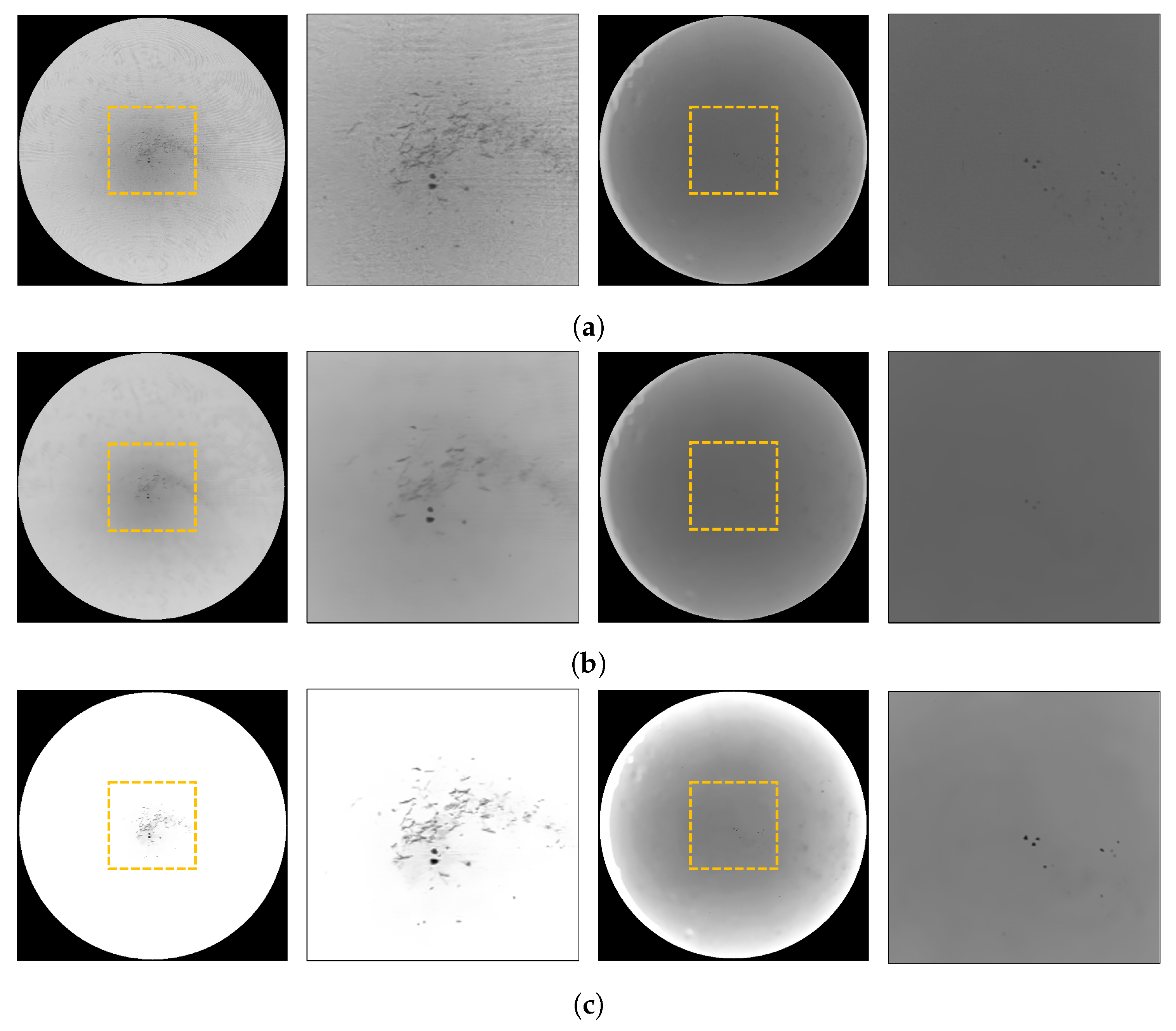
Figure 4.
Moiré removal processes. The left panel is a solution containing undissolved fine particles captured with a Moiré pattern. The right panel is a colored solution containing undissolved fine particles. The yellow box represents the magnification region. (a) The original ROI image. (b) The result of applying the non-local means filter directly to the original ROI image. (c) The result of adjusting the scale and contrast of the original ROI image and applying the non-local means filter.
Figure 5.
Examples that visualize the grid used to calculate the intensity distribution of pixels within the ROI area.
Figure 5.
Examples that visualize the grid used to calculate the intensity distribution of pixels within the ROI area.
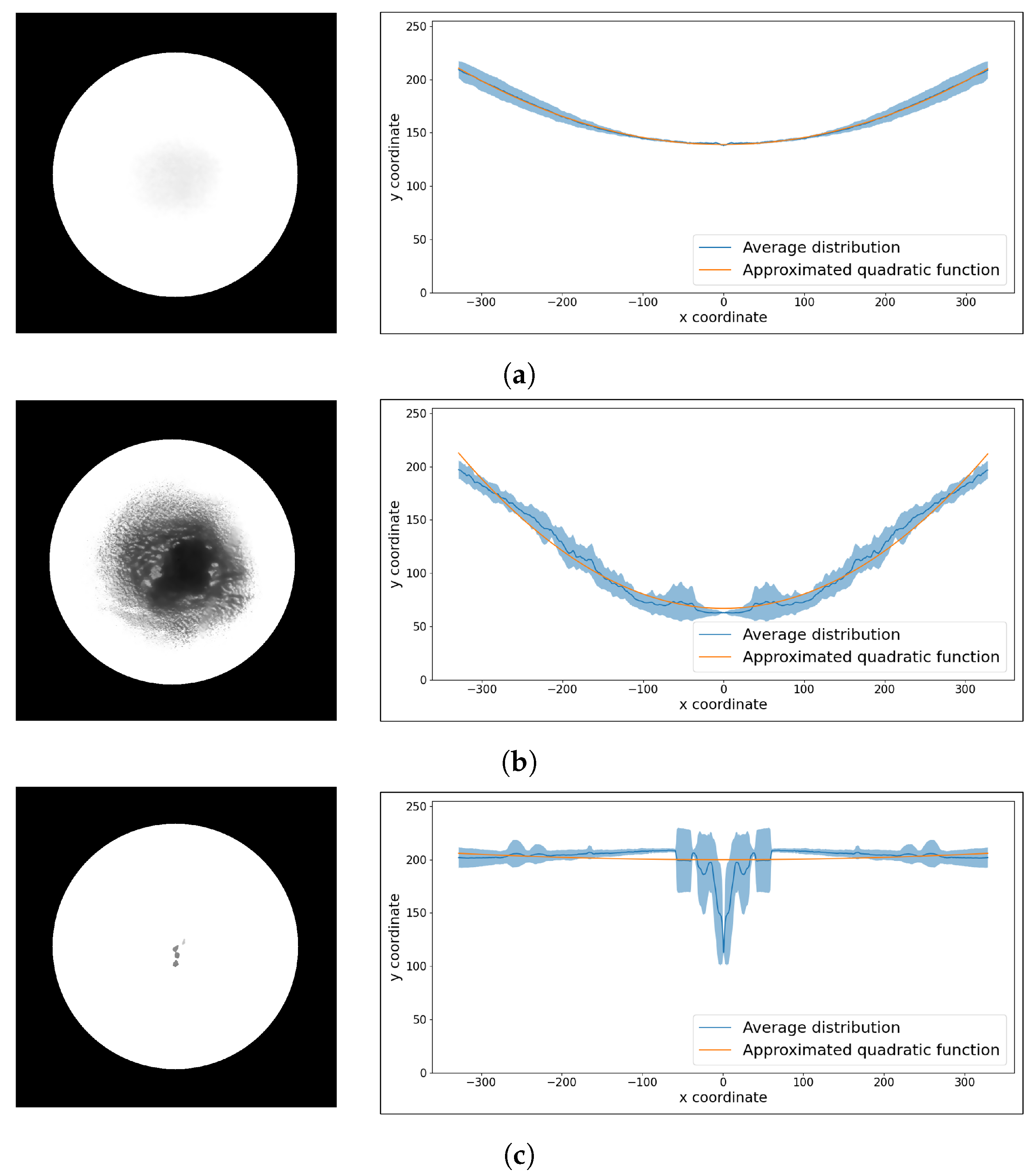
Figure 6.
The left panels show the ROI images of solutions. The radial profile shows the average of the 12 distributions and a quadratic function approximating the average distribution. Additionally, the colored areas correspond to deviations from the 12 distributions. (a) DS, (b) US1, (c) US2 case example.
Figure 7.
A series of PAA processes were performed on a solution with varying amounts of undissolved solute. (a) The ROI image. (b) The result of applying adaptive thresholding. (c) The result of applying a Gabor filter and binary thresholding. (d) The final particle segmentation result.
Figure 7.
A series of PAA processes were performed on a solution with varying amounts of undissolved solute. (a) The ROI image. (b) The result of applying adaptive thresholding. (c) The result of applying a Gabor filter and binary thresholding. (d) The final particle segmentation result.
Figure 8.
For each figure, the left panels show the predicted checked background image using the detected check pattern and the right panels show the superposition result of the predicted checked background image and the detected check pattern. (a) DS, (b) US1, (c) US2 case examples.
Figure 8.
For each figure, the left panels show the predicted checked background image using the detected check pattern and the right panels show the superposition result of the predicted checked background image and the detected check pattern. (a) DS, (b) US1, (c) US2 case examples.
Figure 9.
Examples of training datasets with varying amounts of non-dissolving solutes. (a) CuSO, (b) CuOAc, (c) CuBr, (d) Pd(OAc).
Figure 9.
Examples of training datasets with varying amounts of non-dissolving solutes. (a) CuSO, (b) CuOAc, (c) CuBr, (d) Pd(OAc).
Figure 10.
Examples of the test datasets; (a) 2-bromo-4-phenylpyridine, (b) 4-methoxyphenol, (c) naphthalic anhydride, (d) 4,4′-bis(,-dimethylbenzyl)diphenylamine.
Figure 10.
Examples of the test datasets; (a) 2-bromo-4-phenylpyridine, (b) 4-methoxyphenol, (c) naphthalic anhydride, (d) 4,4′-bis(,-dimethylbenzyl)diphenylamine.
Figure 11.
Equipment used for data acquisition. (a) Equipment modeling, (b) actual equipment.
Figure 11.
Equipment used for data acquisition. (a) Equipment modeling, (b) actual equipment.
Figure 12.
Confusion matrices resulting from ablation studies of DNN on the training dataset. (a) w/o Moiré removal, (b) w/o GHA, (c) w/o RPA, (d) w/o PAA, (e) w/o SA, (f) our method.
Figure 12.
Confusion matrices resulting from ablation studies of DNN on the training dataset. (a) w/o Moiré removal, (b) w/o GHA, (c) w/o RPA, (d) w/o PAA, (e) w/o SA, (f) our method.
Figure 13.
Confusion matrices resulting from ablation studies of DNNs on the test dataset. (a) w/o Moiré removal, (b) w/o GHA, (c) w/o RPA, (d) w/o PAA, (e) w/o SA, (f) our method.
Figure 13.
Confusion matrices resulting from ablation studies of DNNs on the test dataset. (a) w/o Moiré removal, (b) w/o GHA, (c) w/o RPA, (d) w/o PAA, (e) w/o SA, (f) our method.
Figure 14.
Confusion matrices resulting from ablation studies of SVM on the training dataset. (a) w/o Moiré removal, (b) w/o GHA, (c) w/o RPA, (d) w/o PAA, (e) w/o SA, (f) our method.
Figure 14.
Confusion matrices resulting from ablation studies of SVM on the training dataset. (a) w/o Moiré removal, (b) w/o GHA, (c) w/o RPA, (d) w/o PAA, (e) w/o SA, (f) our method.
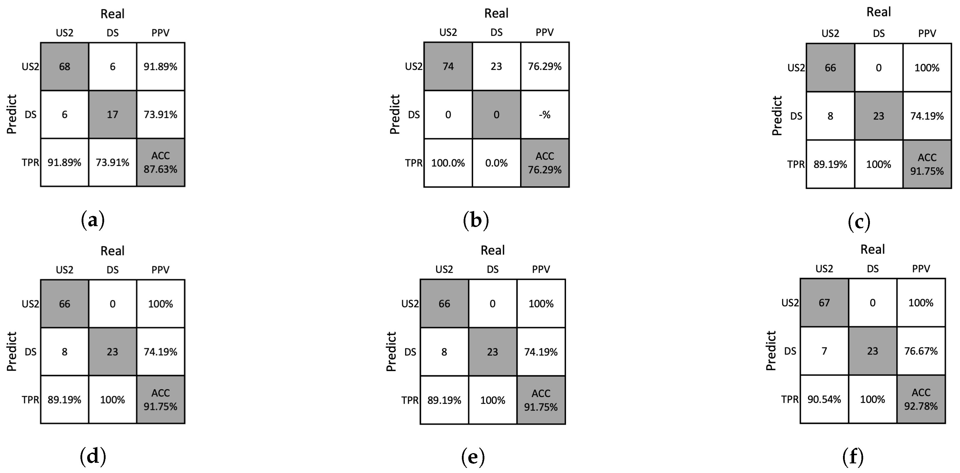
Figure 15.
Confusion matrices resulting from the ablation study of SVM on the test dataset. (a) w/o Moiré removal, (b) w/o GHA, (c) w/o RPA, (d) w/o PAA, (e) w/o SA, (f) our method.
Figure 15.
Confusion matrices resulting from the ablation study of SVM on the test dataset. (a) w/o Moiré removal, (b) w/o GHA, (c) w/o RPA, (d) w/o PAA, (e) w/o SA, (f) our method.
Table 1.
Handcrafted features.
Table 1.
Handcrafted features.
| Feature Name | Background Type | Analysis Method |
|---|
| MMG | White | GHA |
| MSG | White | GHA |
| SMG | White | GHA |
| SSG | White | GHA |
| Minimum value | White | RPA |
| Curvature | White | RPA |
| MSE | White | RPA |
| Number of particles | White | PAA |
| Superposition ratio | Checked | SA |
Table 2.
Combination of the solutes and solvents in the training dataset.
Table 2.
Combination of the solutes and solvents in the training dataset.
| Solute | Solvent | No. Samples |
|---|
| CuSO | DI water | 43 |
| CuOAc | DI water | 41 |
| CuBr | DI water | 30 |
| Pd(OAc) | DI water | 37 |
Table 3.
Combination of solutes and solvents in the test dataset.
Table 3.
Combination of solutes and solvents in the test dataset.
| Solute | Solvent | No. Samples |
|---|
| 2-bromo-4-phenylpyridine | Toluene | 10 |
| 4-Methoxyphenol | Toluene | 65 |
| Naphthalic anhydride | Toluene | 5 |
| Naphthalic anhydride | Methylene chloride | 3 |
| Naphthalic anhydride | Hexane | 2 |
| 4,4′-bis(,-dimethylbenzyl)diphenylamine | Toluene | 12 |
Table 4.
Comparison of various models.
Table 4.
Comparison of various models.
| Model | Training Dataset Acc | Test Dataset Acc | k-Fold Avg Acc |
|---|
| ResNet18 [37] | 98.11 ± 0.43 |
|
|
| ResNet34 [37] |
|
|
|
| InceptionV3 [38] |
|
|
|
| DenseNet121 [39] |
|
|
|
| MobileNetV2 [40] |
|
|
|
| MobileNetV3(small) [41] |
|
|
|
| MobileNetV3(large) [41] |
|
|
|
| ASSNet (Ours) |
|
|
|
Table 5.
Comparison between DNN and SVM.
Table 5.
Comparison between DNN and SVM.
| Model | Training Dataset Acc | Test Dataset Acc | k-Fold Avg Acc |
|---|
| DNN |
|
|
|
| SVM |
|
|
|
Table 6.
Ablation studies on DNN.
Table 6.
Ablation studies on DNN.
| Moiré Removal | GHA | RPA | PAA | SA | Training Dataset Acc | Test Dataset Acc | k-Fold Avg Acc |
|---|
| - | ✓ | ✓ | ✓ | ✓ | 98.34 | 89.69 | 89.29 |
| ✓ | - | ✓ | ✓ | ✓ | 92.22 | 76.29 | 87.78 |
| ✓ | ✓ | - | ✓ | ✓ | 96.52 | 93.81 | 91.52 |
| ✓ | ✓ | ✓ | - | ✓ | 96.85 | 88.66 | 89.80 |
| ✓ | ✓ | ✓ | ✓ | - | 96.19 | 93.81 | 91.61 |
| ✓ | ✓ | ✓ | ✓ | ✓ | 97.68 | 94.85 | 92.12 |
Table 7.
Ablation studies on SVM.
Table 7.
Ablation studies on SVM.
| Moiré Removal | GHA | RPA | PAA | SA | Training Dataset Acc | Test Dataset Acc | k-Fold Avg Acc |
|---|
| - | ✓ | ✓ | ✓ | ✓ | 84.11 | 87.63 | 86.29 |
| ✓ | - | ✓ | ✓ | ✓ | 78.15 | 76.29 | 81.96 |
| ✓ | ✓ | - | ✓ | ✓ | 88.25 | 91.75 | 90.32 |
| ✓ | ✓ | ✓ | - | ✓ | 89.07 | 91.75 | 90.32 |
| ✓ | ✓ | ✓ | ✓ | - | 86.59 | 91.75 | 89.72 |
| ✓ | ✓ | ✓ | ✓ | ✓ | 89.24 | 92.78 | 90.53 |


