

Real-Time Kinematically Synchronous Planning for Cooperative Manipulation of Multi-Arms Robot Using the Self-Organizing Competitive Neural Network


Abstract
1. Introduction
2. Cooperative Manipulation of Multi-Arms
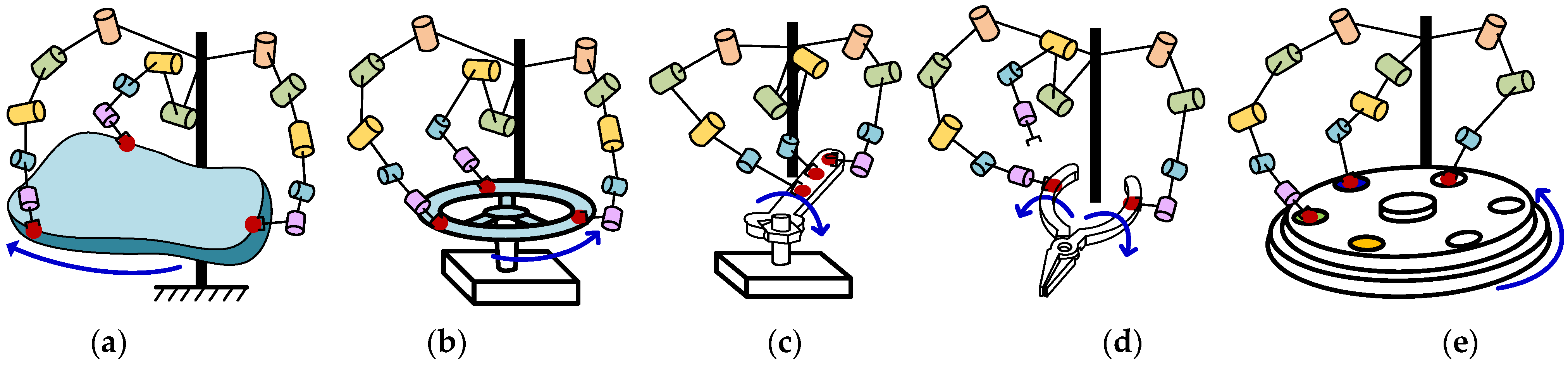
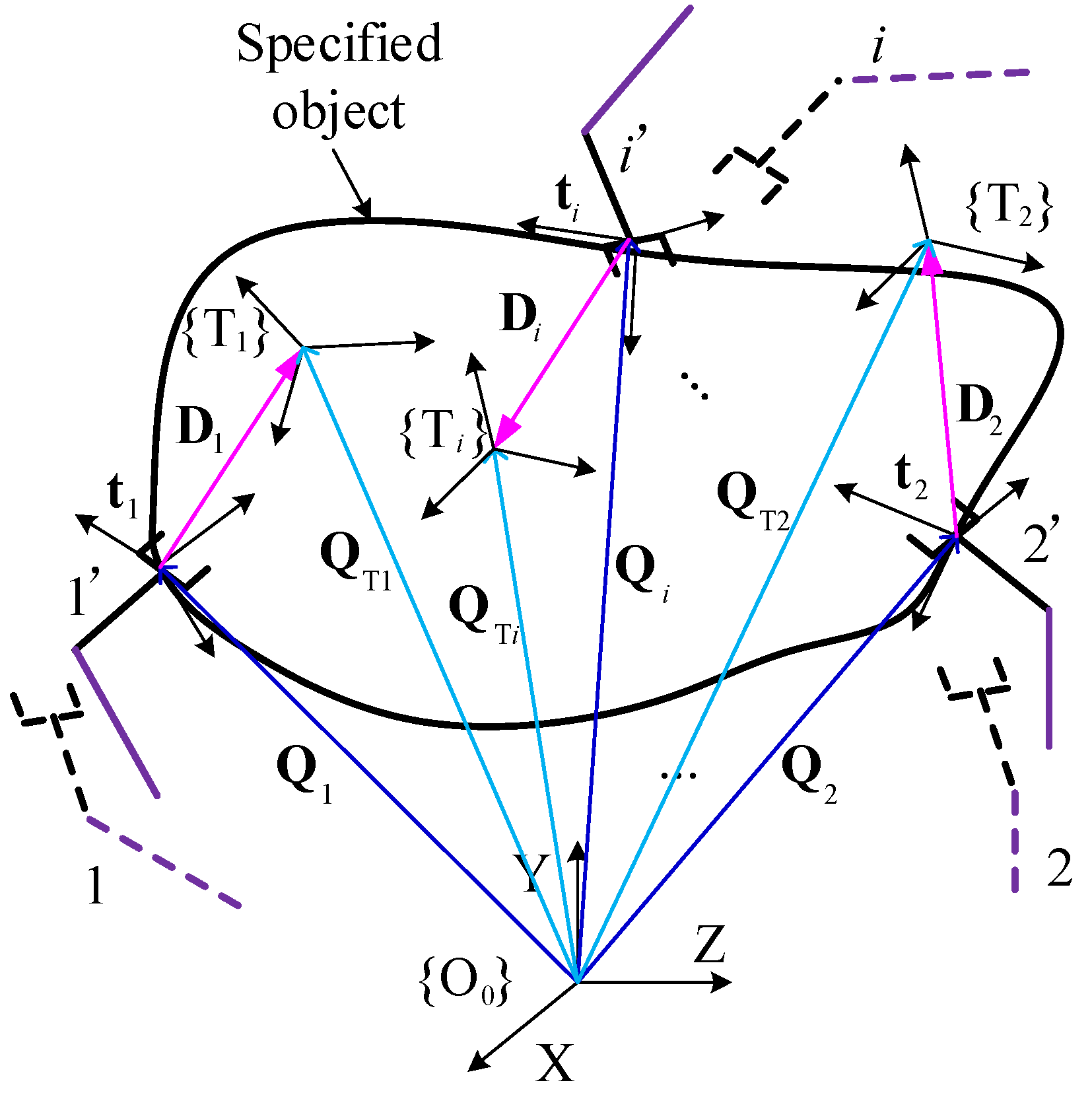
2.1. A Type of Kinematically Cooperative Manipulation
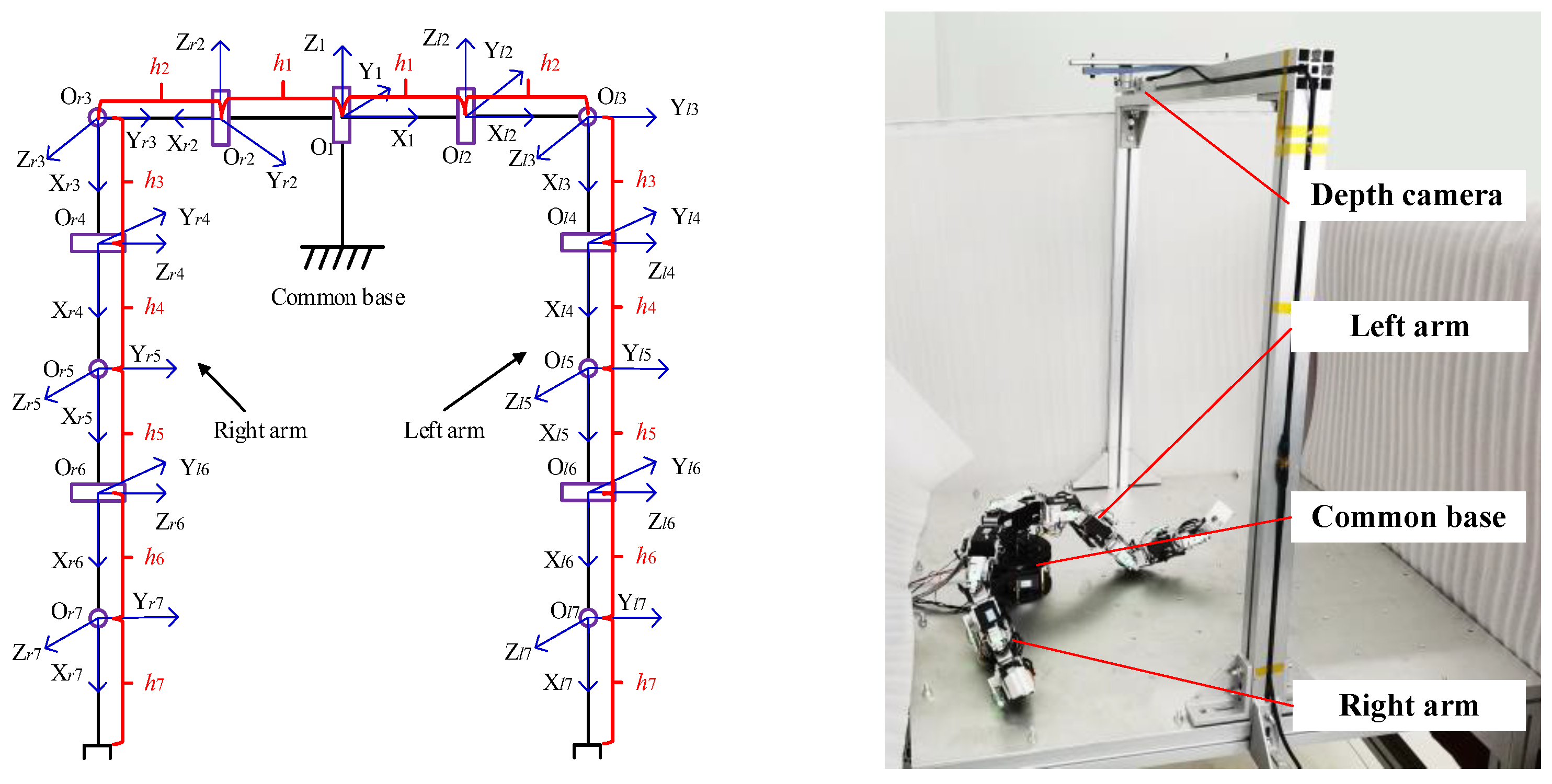
2.2. Multi-Arms Robot with Physical Coupling
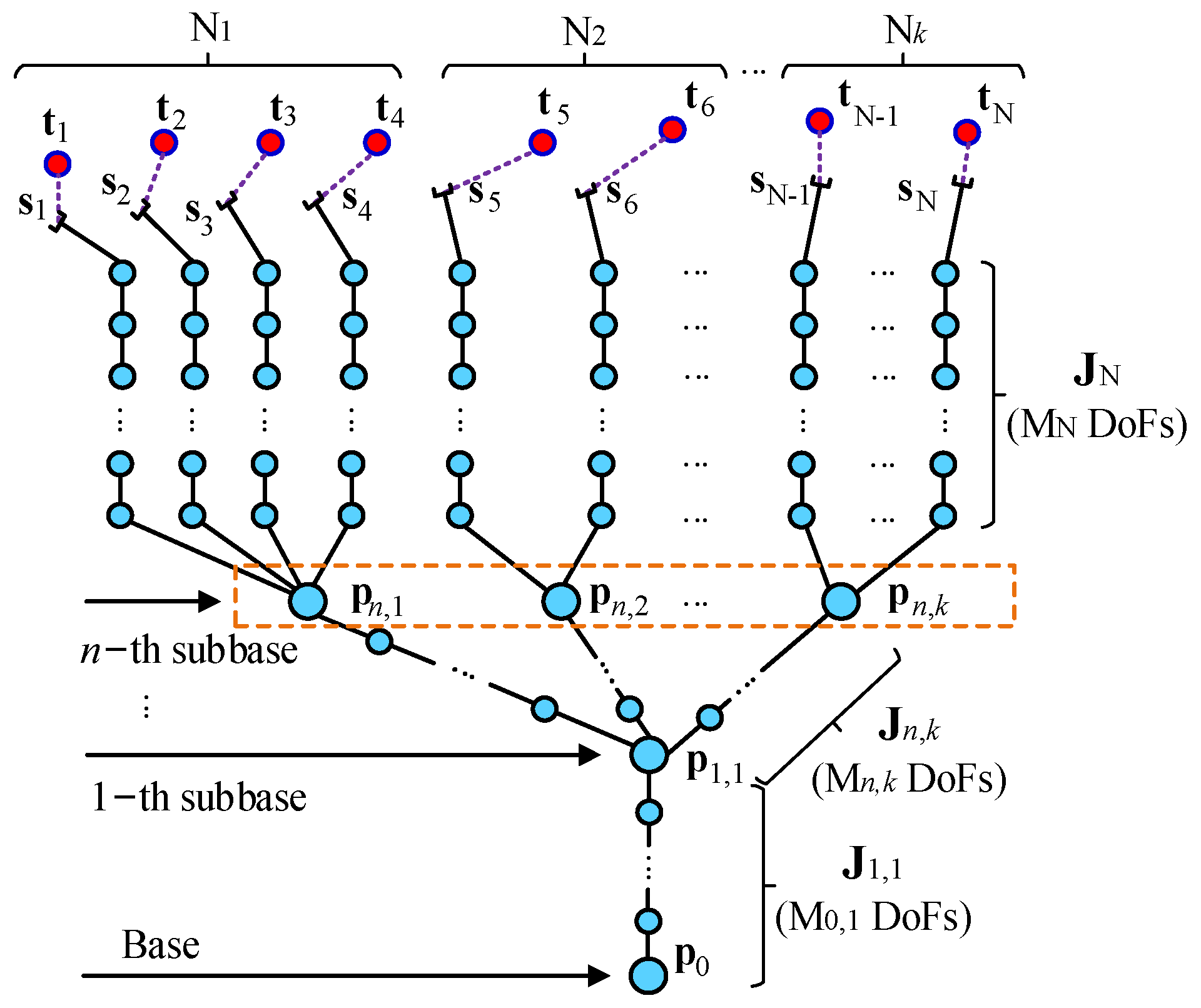
2.3. Definition of Sub-Bases
2.4. Iteration for Multi-Arms Robot Motion
3. Kinematically Synchronous Planning
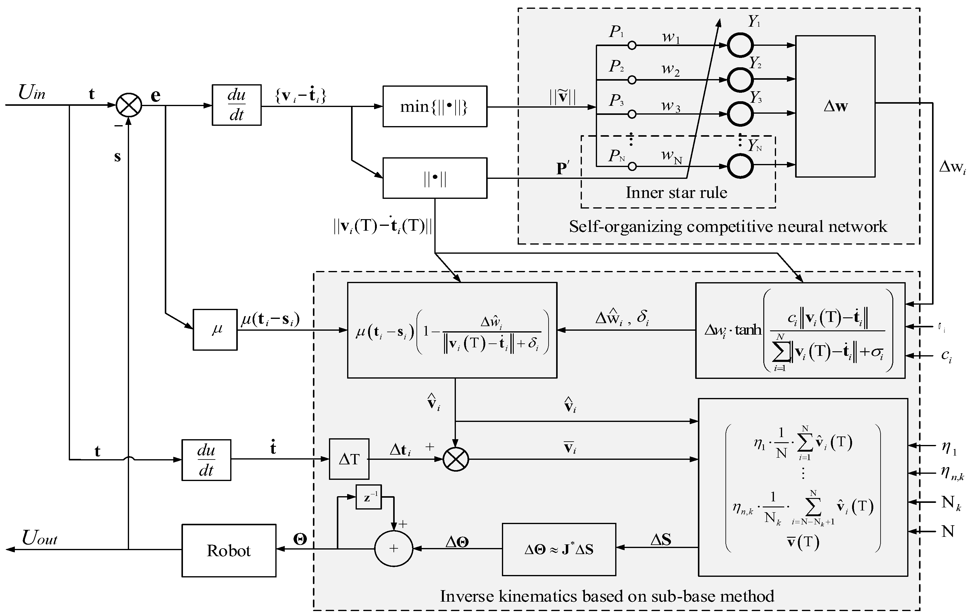
3.1. Synchronous Planning Using Self-Organizing Competitive Neural Network
3.2. Stability Analysis
4. Simulation
5. Experimental Verification
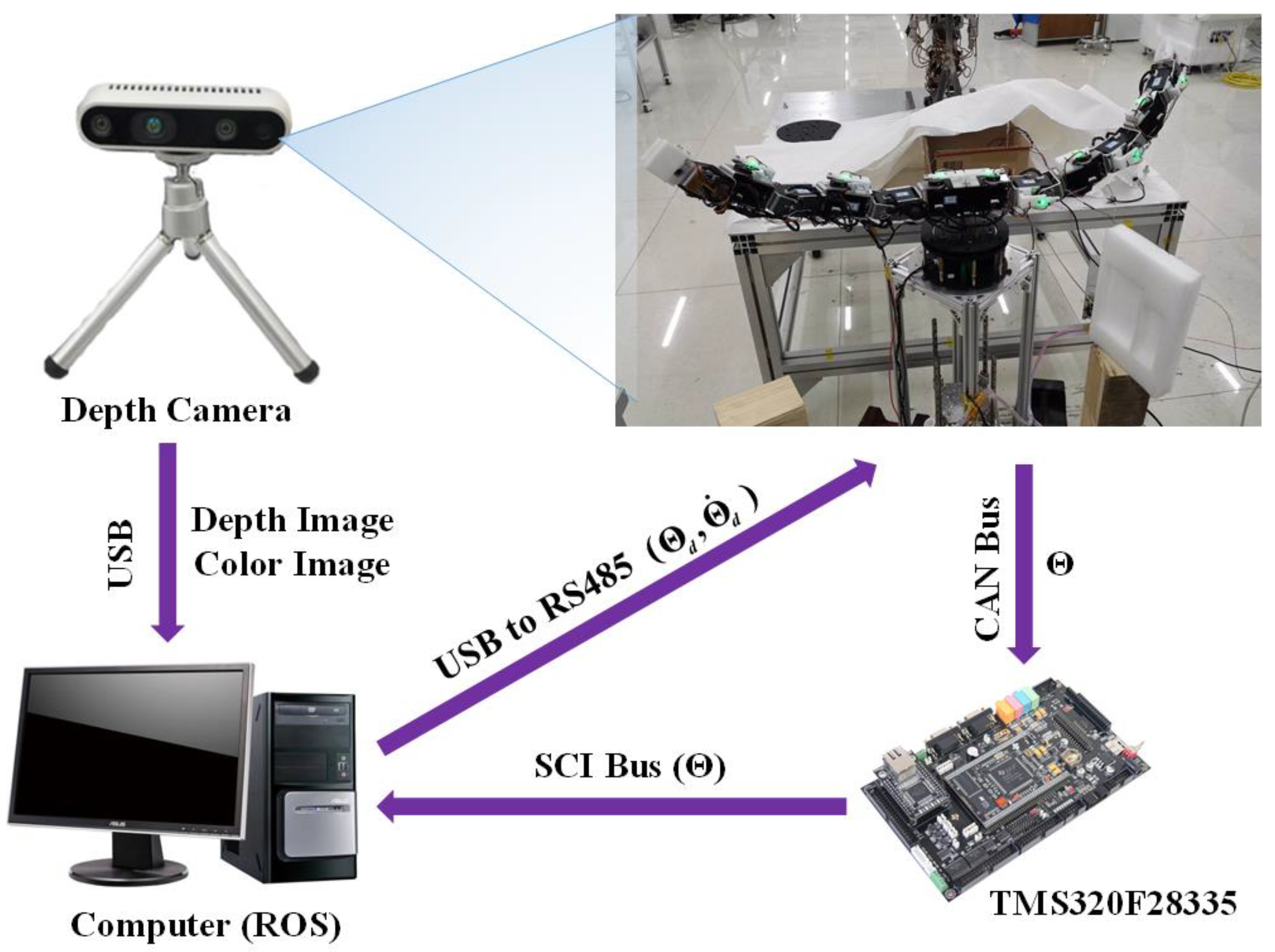
5.1. Experimental Setup
- (1)
- The global depth camera transfers the observed frame of depth and color images to the computer by using a universal serial bus (USB) in real time. The robot operating system (ROS) node runs in the computer and extracts the position information of the object from each frame image. The vision-processing procedures in the computer are developed based on the morphology, using the Open Source Computer Vision Library and the camera Software Development Kit.
- (2)
- The joint feedback data, Θ, of the robot are transmitted to the TMS320F28335 controller through the Controller Area Network (CAN) bus. At the same time, the controller transfers the received joint data, Θ, to the ROS nodes through the Serial Communication Interface (SCI) bus in real time.
- (3)
- The ROS nodes receive the data (xobj, Θ) and execute the forward and inverse kinematics calculation and motion-planning algorithm. The real-time control command data, Θd and , are sent to the robot joint actuator through the RS485 bus to control the motion. The baud rate of the CAN bus, USB serial bus, SCI bus, and RS485 bus is set to 1 MHz. The control period of the whole system containing the proposed kinematically synchronous planning method is less than 10 ms.
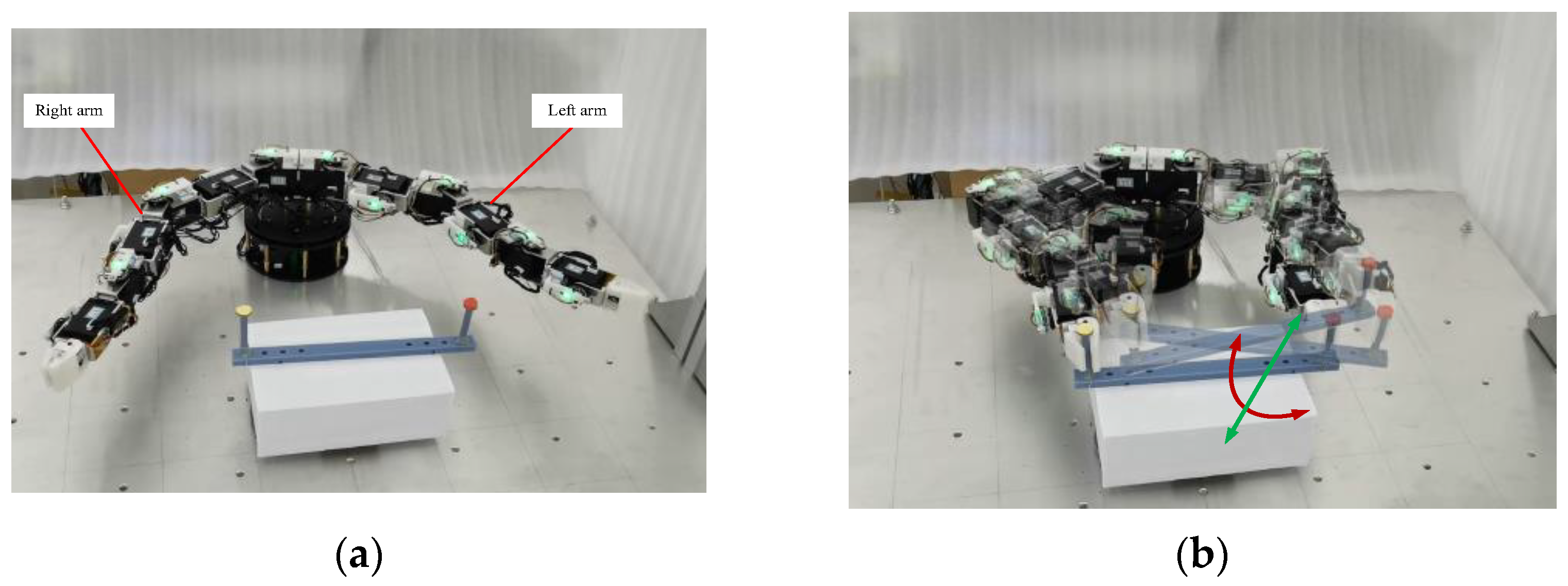
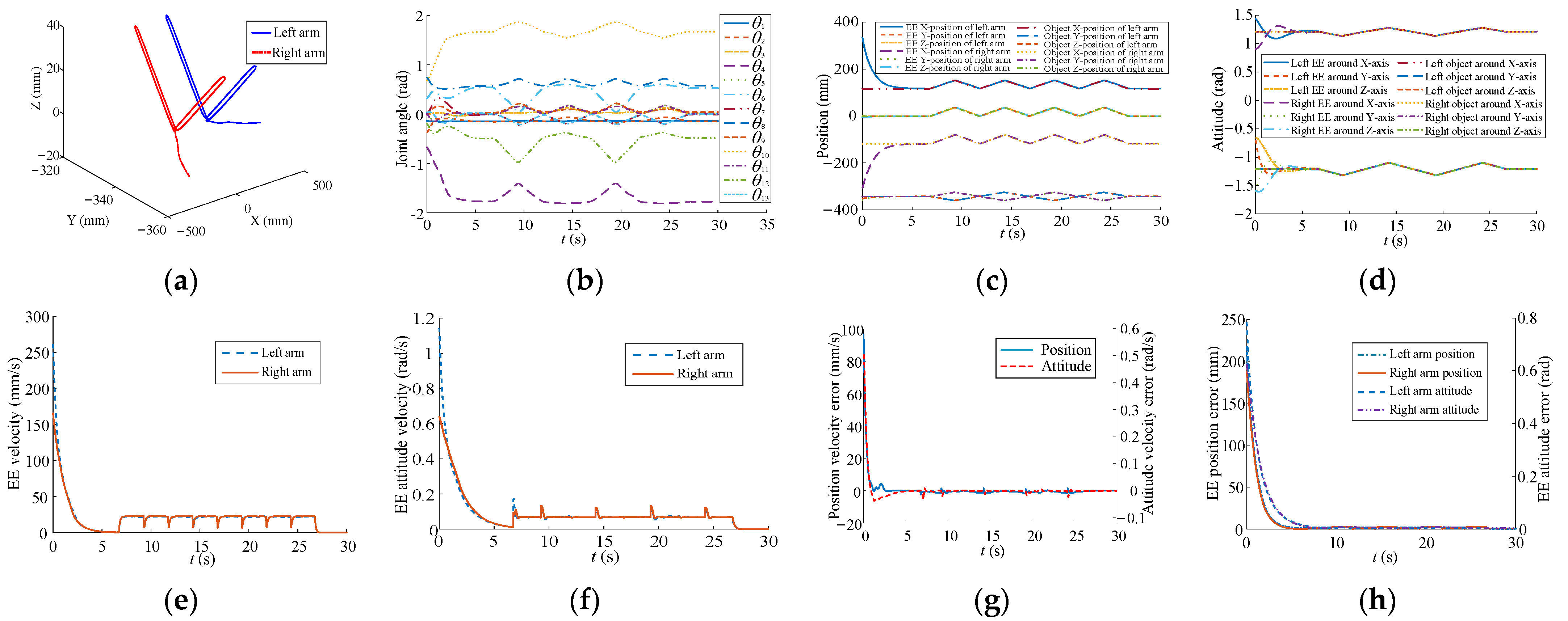
5.2. Synchronous Planning Experiments
- (1)
- Collaboration Carrying
- (2)
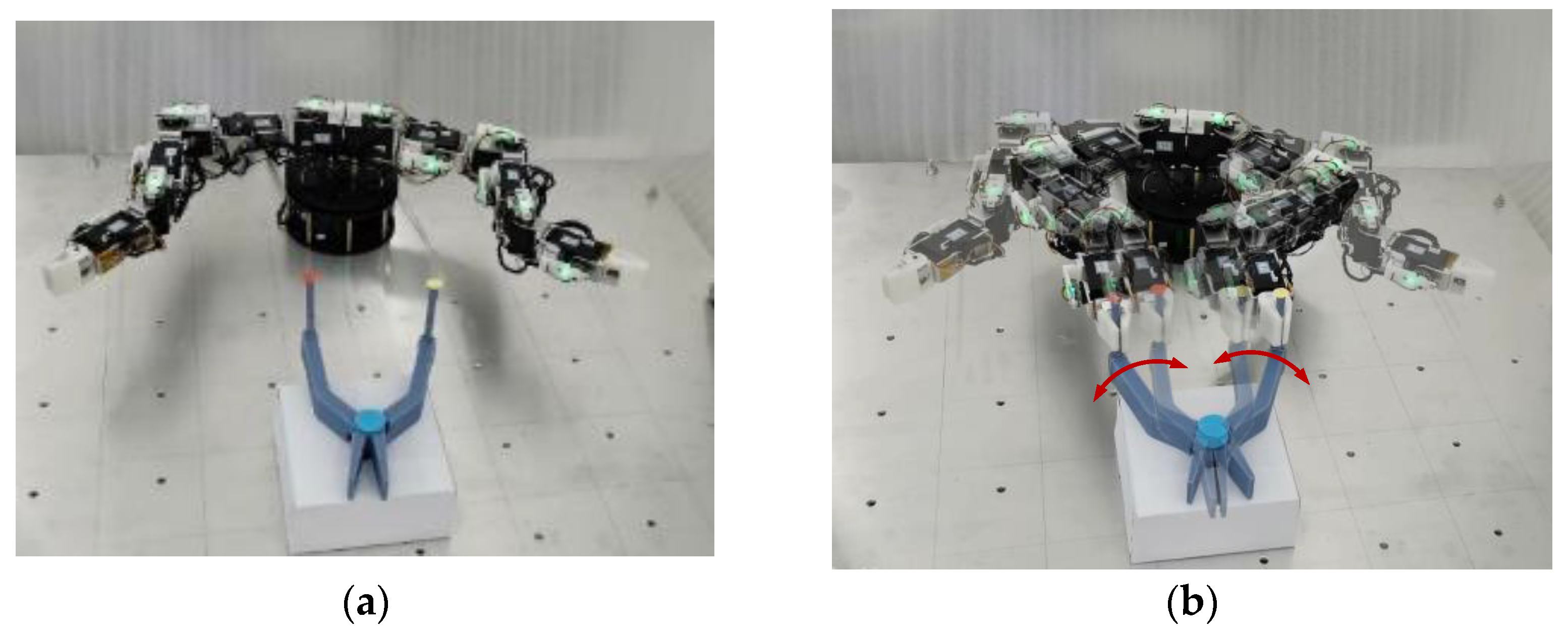
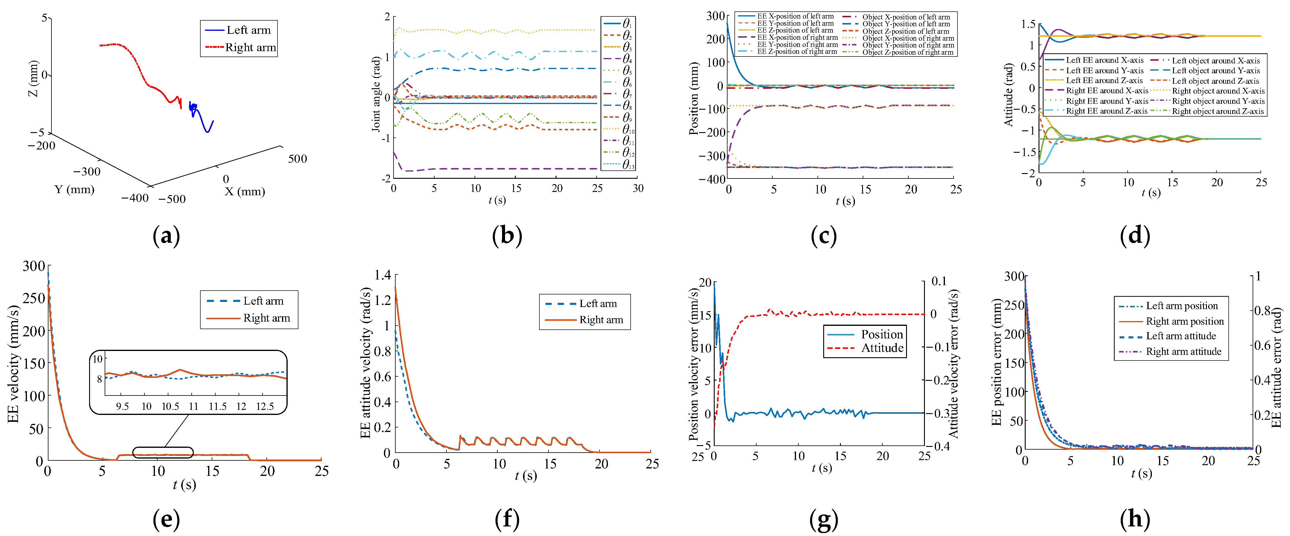
- Manipulating the pliers
- (3)
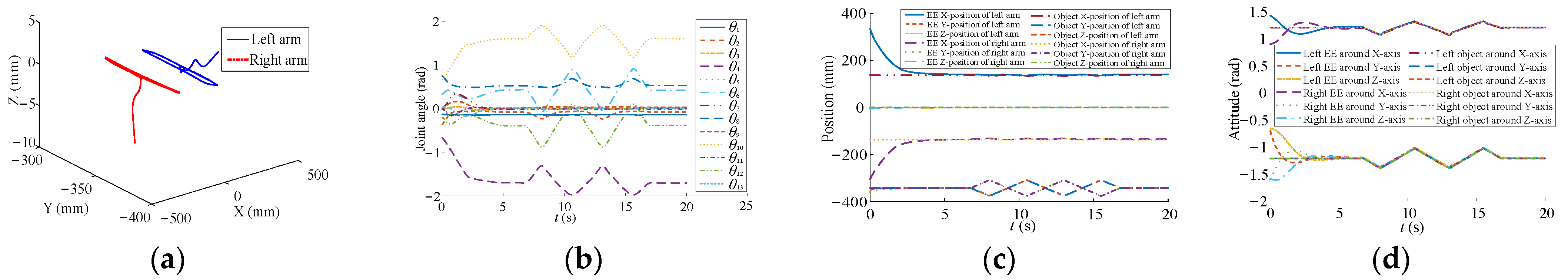
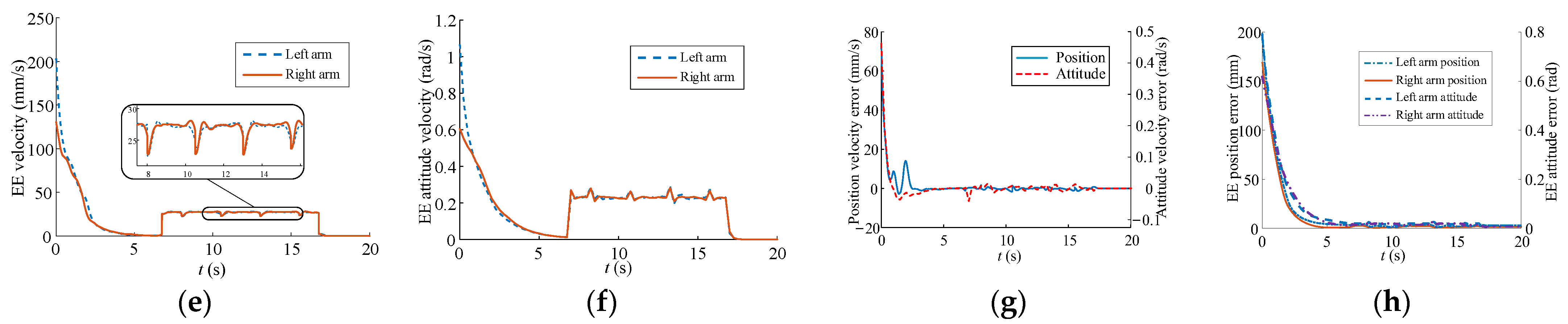
- Manipulating a rudder
6. Conclusions
Author Contributions
Funding
Data Availability Statement
Conflicts of Interest
References
- Li, Z.; Yuan, W.; Zhao, S.; Yu, Z.; Kang, Y.; Chen, C.L.P. Brain-Actuated Control of Dual-Arm Robot Manipulation With Relative Motion. IEEE Trans. Cogn. Dev. Syst. 2019, 11, 51–62. [Google Scholar] [CrossRef]
- Yang, C.; Chen, C.; Wang, N.; Ju, Z.; Fu, J.; Wang, M. Biologically Inspired Motion Modeling and Neural Control for Robot Learning From Demonstrations. IEEE Trans. Cogn. Dev. Syst. 2019, 11, 281–291. [Google Scholar]
- Nicolis, D.; Palumbo, M.; Zanchettin, A.M.; Rocco, P. Occlusion-Free Visual Servoing for the Shared Autonomy Teleoperation of Dual-Arm Robots. IEEE Robot. Autom. Lett. 2018, 3, 796–803. [Google Scholar] [CrossRef]
- Schmaus, P.; Leidner, D.; Bayer, R.; Pleintinger, B.; Krüger, T.; Lii, N.Y. Continued Advances in Supervised Autonomy User Interface Design for METERON SUPVIS Justin. In Proceedings of the 2019 IEEE Aerospace Conference, Big Sky, MT, USA, 2–9 March 2019; pp. 1–11. [Google Scholar]
- Ambrose, R.; Savely, R.; Goza, S.; Strawser, P.; Radford, N. Mobile Manipulation using NASA’s Robonaut. In Proceedings of the IEEE International Conference on Robotics and Automation, New Orleans, LA, USA, 26 April–1 May 2004; Volume 2, pp. 2104–2109. [Google Scholar]
- Chen, B.; Wang, Y.; Lin, P. A Hybrid Control Strategy for Dual-arm Object Manipulation Using Fused Force/Position Errors and Iterative Learning. In Proceedings of the 2018 IEEE/ASME International Conference on Advanced Intelligent Mechatronics (AIM), Auckland, New Zealand, 9–12 July 2018; pp. 39–44. [Google Scholar]
- Nozawa, S.; Kakiuchi, Y.; Okada, K.; Inaba, M. Controlling the Planar Motion of a Heavy Object by Pushing with a Humanoid Robot using Dual-Arm Force Control. In Proceedings of the 2012 IEEE International Conference on Robotics and Automation, Saint Paul, MN, USA, 14–18 May 2012; pp. 1428–1435. [Google Scholar]
- Suarez, A.; Heredia, G.; Ollero, A. Physical-Virtual Impedance Control in Ultralightweight and Compliant Dual-Arm Aerial Manipulators. IEEE Robot. Autom. Lett. 2018, 3, 2553–2560. [Google Scholar] [CrossRef]
- Lee, J.; Chang, P.H.; Jamisola, R.S. Relative Impedance Control for Dual-Arm Robots Performing Asymmetric Bimanual Tasks. IEEE Trans. Ind. Electron. 2014, 61, 3786–3796. [Google Scholar] [CrossRef]
- Kong, L.; He, W.; Yang, C.; Li, Z.; Sun, C. Adaptive Fuzzy Control for Coordinated Multiple Robots With Constraint Using Impedance Learning. IEEE T. Cybern. 2019, 49, 3052–3063. [Google Scholar] [CrossRef] [PubMed]
- Zhang, Z.; Lin, Y.; Li, S.; Li, Y.; Yu, Z.; Luo, Y. Tricriteria Optimization-Coordination Motion of Dual-Redundant-Robot Manipulators for Complex Path Planning. IEEE Trans. Control Syst. Technol. 2018, 26, 1345–1357. [Google Scholar] [CrossRef]
- Li, X.; Tan, S.; Feng, X.; Rong, H. LSPB Trajectory Planning: Design for the Modular Robot Arm Applications. In Proceedings of the 2009 International Conference on Information Engineering and Computer Science, Wuhan, China, 19–20 December 2009; pp. 1–4. [Google Scholar]
- Bouteraa, Y.; Ghommam, J.; Poisson, G. Adaptive Backstepping Synchronization for Networked Lagrangian Systems. Int. J. Comput. Appl. Technol. 2012, 42, 1–8. [Google Scholar] [CrossRef]
- Uchiyama, M.; Dauchez, P. Symmetric Kinematic Formulation and Non-master/Slave Coordinated Control of Two-Arm Robots. Adv. Robot. 1992, 7, 361–383. [Google Scholar] [CrossRef]
- Caccavale, F.; Chiacchio, P.; Chiaverini, S. Task-Space Regulation of Cooperative Manipulators. Automatica 2000, 36, 879–887. [Google Scholar] [CrossRef]
- Adorno, B.; Fraisse, P.; Druon, S. Dual Position Control Strategies Using the Cooperative Dual Task-Space Framework. In Proceedings of the 2010 IEEE/RSJ International Conference on Intelligent Robots and Systems, Taipei, Taiwan, 18–22 October 2010; pp. 3955–3960. [Google Scholar]
- Park, H.; Lee, C. Cooperative-Dual-Task-Space-based Whole-Body Motion Balancing for Humanoid Robots. In Proceedings of the 2013 IEEE International Conference on Robotics and Automation, Karlsruhe, Germany, 6–10 May 2013; pp. 4797–4802. [Google Scholar]
- Park, H.; Lee, C. Extended Cooperative Task Space for Manipulation Tasks of Humanoid Robots. In Proceedings of the 2015 IEEE International Conference on Robotics and Automation (ICRA), Seattle, WA, USA, 26–30 May 2015; pp. 6088–6093. [Google Scholar]
- Park, H.; Lee, C. Dual-Arm Coordinated-Motion Task Specification and Performance Evaluation. In Proceedings of the 2016 IEEE/RSJ International Conference on Intelligent Robots and Systems (IROS), Daejeon, Republic of Korea, 9–14 October 2016; pp. 929–936. [Google Scholar]
- Basile, F.; Caccavale, F.; Chiacchio, P.; Coppola, J.; Marino, A. A Decentralized Kinematic Control Architecture for Collaborative and Cooperative Multi-Arm Systems. Mechatronics 2013, 23, 1100–1112. [Google Scholar] [CrossRef]
- Basile, F.; Caccavale, F.; Chiacchio, P.; Coppola, J.; Curatella, C. Task-Oriented Motion Planning for Multi-Arm Robotic Systems. Robot. Comput.-Integr. Manuf. 2012, 28, 569–582. [Google Scholar] [CrossRef]
- Zhang, Z.; Kong, L.; Niu, Y. A Time-Varying-Constrained Motion Generation Scheme for Humanoid Robot Arms. In Advances in Neural Networks; Springer: Berlin/Heidelberg, Germany, 2018; Volume 10878, pp. 757–767. [Google Scholar]
- Curkovic, P.; Jerbic, B. Dual-arm Robot Motion Planning based on Cooperative Coevolution. Emerg. Trends Technol. Innov. 2010, 314, 169–178. [Google Scholar]
- Caccavale, F.; Lippiello, V.; Muscio, G.; Pierri, F.; Ruggiero, F.; Villani, L. Grasp Planning and Parallel Control of A Redundant Dual-Arm/Hand Manipulation System. Robotica 2013, 31, 1169–1194. [Google Scholar] [CrossRef]
- Stavridis, S.; Doulgeri, Z. Bimanual Assembly of Two Parts with Relative Motion Generation and Task Related Optimization. In Proceedings of the 2018 IEEE/RSJ International Conference on Intelligent Robots and Systems (IROS), Madrid, Spain, 1–5 October 2018; pp. 7131–7136. [Google Scholar]
- Almeida, D.; Karayiannidis, Y. A Lyapunov-Based Approach to Exploit Asymmetries in Robotic Dual-Arm Task Resolution. In Proceedings of the 2019 IEEE 58th Conference on Decision and Control (CDC), Nice, France, 3 May 2019; pp. 4252–4258. [Google Scholar]
- Jin, T.; Xia, H. Lookback Option Pricing Models Based on the Uncertain Fractional-Order Differential Equation with Caputo Type. J. Ambient Intell. Hum. Comput. 2021, 14, 6435–6448. [Google Scholar] [CrossRef]
- Zhang, S.; Cao, Y. Consensus in Networked Multi-robot Systems Via Local State Feedback Robust Control. Int. J. Adv. Robot Syst. 2019, 16, 45–52. [Google Scholar] [CrossRef]
- Zhang, S.; Cao, Y. Cooperative Localization Approach for Multi-Robot Systems Based on State Estimation Error Compensation. Sensors 2019, 19, 3842. [Google Scholar] [CrossRef] [PubMed]
- Aristidou, A.; Lasenby, J. Inverse Kinematics: A Review of Existing Techniques and Introduction of a New Fast Iterative Solver; Technical Report; Cambridge University Engineering Department: Cambridge, UK, 2009. [Google Scholar]
- Buss, S.R.; Kim, J.-S. Selectively Damped Least Squares for Inverse Kinematics. J. Graph. Tools 2005, 10, 37–49. [Google Scholar] [CrossRef]


| li | 1 | 2 | 3 | 4 | 5 |
| Length (m) | 1.18 | 0.88 | 0.88 | 0.88 | 0.88 |
| li | 6 | 7 | 8 | 9 | 10 |
| Length (m) | 0.88 | 57.85 | 0.88 | 0.88 | 0.88 |
| li | 11 | 12 | 13 | 14 | 15 |
| Length (m) | 57.85 | 0.88 | 0.88 | 0.88 | 57.85 |
| 1 | 2 | 3 | 4 | 5 | |
| Initial angle (°) | −5.0 | 5.0 | 5.0 | 30.0 | 20.0 |
| 6 | 7 | 8 | 9 | 10 | |
| Initial angle (°) | 20.0 | 20.0 | −70.0 | 20.0 | 20.0 |
| 11 | 12 | 13 | 14 | 15 | |
| Initial angle (°) | 20.0 | 10.0 | 10.0 | 20.0 | 20.0 |
| Parameters | μ | N | b | R | ||
| Value | 0.08 | 1/6 | 3 | 3 | 1 | 15 |
| Parameters | M0,1 | M1 | M2 | M3 | λ | |
| Value | 3 | 4 | 4 | 4 | 0.01 | 0.05 |
| i | (mm) | (rad) | i | (mm) | (rad) | ||||||
|---|---|---|---|---|---|---|---|---|---|---|---|
| Left Arm | 1 | 0 | = 42 | 0 | 0 | Right Arm | 1 | 0 | = 42 | π | 0 |
| 2 | 0 | h2 = 84 | π/2 | 0 | 2 | 0 | = 84 | π/2 | 0 | ||
| 3 | 0 | = 84 | −π/2 | 0 | 3 | 0 | = 84 | −π/2 | 0 | ||
| 4 | 0 | = 84 | π/2 | 0 | 4 | 0 | = 84 | π/2 | 0 | ||
| 5 | 0 | = 78 | −π/2 | 0 | 5 | 0 | = 78 | −π/2 | 0 | ||
| 6 | 0 | h7 = 71 | π/2 | 0 | 6 | 0 | = 71 | π/2 | 0 | ||
| 7 | 0 | = 71 | 0 | 0 | 7 | 0 | = 71 | 0 | 0 |
| Parameters | μ | N | b | r | ||
| Value | 0.005 | 5 | 2 | 2 | 1 | 13 |
| Parameters | M0,1 | M1 | M2 | λ | — | |
| Value | 1 | 6 | 6 | 0.01 | 0.05 | — |
| Parameters | ||||
| Value | 1 × 10⁻⁵ | 1 × 10⁻⁵ | 2.0 | 0.03 |
Disclaimer/Publisher’s Note: The statements, opinions and data contained in all publications are solely those of the individual author(s) and contributor(s) and not of MDPI and/or the editor(s). MDPI and/or the editor(s) disclaim responsibility for any injury to people or property resulting from any ideas, methods, instructions or products referred to in the content. |
© 2023 by the authors. Licensee MDPI, Basel, Switzerland. This article is an open access article distributed under the terms and conditions of the Creative Commons Attribution (CC BY) license (https://creativecommons.org/licenses/by/4.0/).
Share and Cite
Zhang, H.; Jin, H.; Ge, M.; Zhao, J. Real-Time Kinematically Synchronous Planning for Cooperative Manipulation of Multi-Arms Robot Using the Self-Organizing Competitive Neural Network. Sensors 2023, 23, 5120. https://doi.org/10.3390/s23115120
Zhang H, Jin H, Ge M, Zhao J. Real-Time Kinematically Synchronous Planning for Cooperative Manipulation of Multi-Arms Robot Using the Self-Organizing Competitive Neural Network. Sensors. 2023; 23(11):5120. https://doi.org/10.3390/s23115120
Chicago/Turabian StyleZhang, Hui, Hongzhe Jin, Mingda Ge, and Jie Zhao. 2023. "Real-Time Kinematically Synchronous Planning for Cooperative Manipulation of Multi-Arms Robot Using the Self-Organizing Competitive Neural Network" Sensors 23, no. 11: 5120. https://doi.org/10.3390/s23115120
APA StyleZhang, H., Jin, H., Ge, M., & Zhao, J. (2023). Real-Time Kinematically Synchronous Planning for Cooperative Manipulation of Multi-Arms Robot Using the Self-Organizing Competitive Neural Network. Sensors, 23(11), 5120. https://doi.org/10.3390/s23115120