1. Introduction
Several sensors aim at estimating the direction of arrival (DoA) of narrowband signals exploit linear antenna arrays with a small number of receiving elements. This choice allows for the minimizing of the number of receiving channels and the reducing of the overall system complexity, enabling the design of low-cost, lightweight, and compact sensors which are suitable for the mass-market.
Among the many applications that could benefit from a small number of receiving channels are low-cost radars for vehicular anti-collision applications—which estimate the direction of the target echo passive sonar systems—as well as passive radar (PR) systems [
1], usually characterized by low-cost requirements compared to their active counterparts. Specifically, PRs based on different RF waveforms of opportunity have been widely studied. For example, considering the drone detection application, encouraging results have been obtained by parasitically exploiting a variety of RF waveforms, such as GSM [
2], UMTS [
3], LTE [
4], DVB-T [
5,
6,
7,
8,
9], and Wi-Fi signals [
10,
11].
Furthermore, low-cost sensors are particularly attractive in civil surveillance applications, e.g., PR sensors for the surveillance of private facilities [
12], passive location sensors for the indoor monitoring of human activity [
13], and sensors for the localization of survivors during the search and rescue operations after natural disasters. For all these applications, cost containment, limited complexity, and system lightness are crucial features. Therefore, the number of employed antenna elements and receiving channels must be kept as low as possible.
Three-element array configurations are currently widely considered for the practical, cost-effective implementation of limited beamforming and/or DoA estimation capability. As an example, the application for radio science experiments is presented in [
14], whereas an example for 5G applications is reported in [
15] for the C-band case using a uniform linear array (ULA) configuration with a pre-assigned element distance. Reference [
16] presents the design and measurements of a 122 GHz on-chip patch antenna array in a 130 nm SiGe BiCMOS technology. The array is formed by three rectangular patches in the top metallization layer, with the ground plane in the lowest layer. Reference [
17] presents a 300 GHz three-element on-chip patch antenna for applications in broadband Sub-THz communication and high-resolution radar sensing. The practical interest regarding the three-element array case also suggested the investigation of the possibility of removing the undesired e.m. coupling among its elements [
18].
As pointed out in [
19], when dealing with DoA estimation, two main reasons motivate the designer to use inter-element distances greater than
λ/2, especially when using a small number of receiving channels:
Achieving a longer global array length, thus improving DoA estimation accuracy;
Attaining compliance with technological constraints (e.g., the antenna element size might set a minimum inter-element distance).
Recently, significant efforts have been invested in the optimization of this simple, but useful, configuration. Unfortunately, it is well known that when estimating the DoA in an angular sector
, a ULA is affected by deterministic angular ambiguities if the uniform spacing between adjacent antenna elements exceeds
. In particular, in reference [
20], the binomial weight configuration is used, and both the element distance and the array factor are selected for a specific case.
In contrast, a non-uniform linear array (NULA) is only affected by statistical ambiguities, whose impact largely depends on the available signal-to-noise power ratio (
). The use of NULA configurations has been explored in [
21,
22].
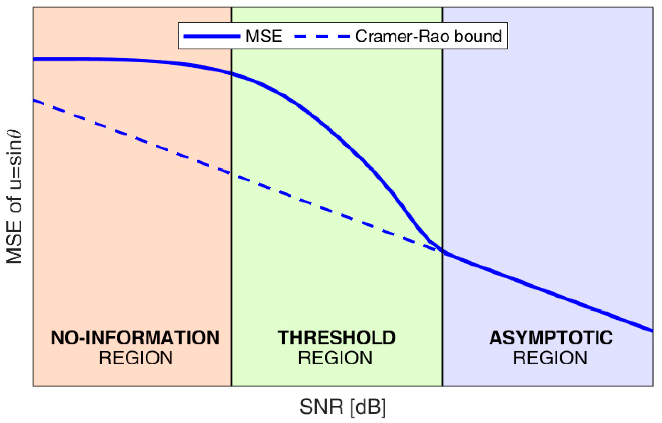
Specifically, under very high
conditions, the NULA estimation accuracy reaches the Cramer–Rao bound (
), which essentially depends on the global array length. In this
region, known as asymptotic region, the estimation variance is inversely proportional to the
. However, below a specific
value, the presence of statistical ambiguities results in large estimation errors, also known as outliers, occurring with a non-negligible probability. Several authors addressed this issue in literature [
23,
24,
25,
26,
27], exploring the use of different lower bounds, such as the Ziv-Zakai bound [
27]. In this range of
values, known as the threshold region, the outlier probability monotonically grows as the
decreases, while the DoA estimation variance rapidly deviates from the
.
Therefore, a design strategy to select the optimal NULA configuration is particularly attractive, since the operational application of the previously introduced low-cost sensors typically faces limited
conditions. The design strategy proposed in [
28] provides useful guidelines to select a proper array configuration. However, only antenna spacings in multiples of
are considered, which in turn leads to the following two weaknesses:
Depending on the value and on the angular sector of interest, there is no guarantee that using inter-element distances with quantization provides the optimal solution;
Depending on the physical size of the employed antennas, operating with half-wavelength quantization may strongly limit the available design solutions, making the technological constraint more severe.
Moreover, it is unlikely that the quantized element spacing will allow for the investigation of the impact of the element positioning tolerance due to practical installation and/or manufacturing.
Array layout design approaches based on the symmetrical number system were proposed in [
29,
30], using an optimum symmetrical number system (OSNS) and a robust symmetrical number system (RSNS) of a pairwise relatively prime number, respectively. However, these design strategies do not provide a control of the performance in terms of statistical ambiguity resolution. More interestingly, an array spacing design procedure was presented in [
31] for three- and four-elements arrays, including a constraint on a maximum admissible phase error in the design procedure, which allows for the exclusion of arrays that provide DoA ambiguity if the phase error exceeds a preassigned value. This approach can be considered as a first step towards our proposed design approach. In fact, in the following, we present an array spacing design procedure for the three-elements case that includes a direct control over the statistics of the ambiguity resolution. We fully characterize the probability of ambiguity resolution and provide an array spacing design procedure that guarantees a preassigned probability.
Specifically, based on the theoretical characterization of the DoA estimation error carried out by the author of [
32], the proposed design strategy provides an array configuration which is not subject to the quantization constraint on the inter-element distance. The findings in [
32] allow us to devise a procedure that constrains the searched NULA array configurations to provide an outlier probability below a maximum tolerable value. Moreover, the prediction of the maximum likelihood estimator (MLE) performance provided therein, in both the threshold and asymptotic regions, enables the identification of the solution with minimum mean square error (MSE), even for limited values of the available
. This also allows us to include additional constraints related to practical array manufacturing. It is interesting to note that design approaches for arrays with more than three elements were proposed in [
33,
34] as evolutions or combinations of the three-elements array procedures. Therefore, the contribution of this paper is also expected to provide useful elements for the design of longer arrays.
The remainder of the paper is organized as follows. In
Section 2, the signal model, DoA MLE, and theoretical characterization of the MSE are introduced. In
Section 3, the admissible pairwise probability (APP) region is defined as the parameters region containing the arrays that satisfy the constraint on the maximum outlier probability for a chosen
. Based on the APP region, the design strategy is derived as a constrained optimization problem and is presented in
Section 4. In
Section 5, a numerical analysis is carried out to assess the performance of various NULA configurations obtained with the proposed strategy. A comparison with the design strategy proposed in [
27] is also carried out to show the limitations of the quantization constraint.
Section 6 shows the benefits of the proposed strategy over the conventional approach when adding technological constraints, which further limits the available array configurations. Finally, in
Section 7, the advantages shown for the simulated data are tested against an experimental dataset collected in the Wi-Fi band. Concluding remarks are reported in
Section 8.
3. Admissible Pairwise Probability Region
From the approximation in Equation (7), we notice that the values of act as scaling factors for the large error contributions that add to the to provide the global MSE. Therefore, the array configuration achieving the minimum MSE certainly lies in a region where the pairwise probabilities have negligible values. Consequently, an important step toward the array optimization consists of the identification of the region of the array parameters, namely , where all values are below an assigned threshold (i.e., the maximum acceptable value). This region will be referred to in the following as the APP region.
To identify the APP region, we notice that the th pairwise error probability in Equation (9) is a monotonic decreasing function of both the and the array beampattern evaluated at the th sidelobe peak location . Therefore, the array configuration achieving the minimum MSE depends on the specific conditions. To carry out the optimization, we first select a fixed value for the , i.e., . With this choice, the constraint on is equivalent to setting an upper bound on the value of , namely , where ).
By using the steering vector in Equation (1), the likelihood function
in Equation (5) can be expressed in terms of the array parameters
:
where
While this constraint is valid for any value of
, we are especially interested to the case of
, which is appealing when addressing the design of low-cost, lightweight sensors, as described in the
Section 1. For
array elements, the constraint in Equation (11) can be simplified as:
which is a function of two parameters and can be easily represented in a plane.
Figure 3 shows a contour plot representing the function
on a
axis system.
Notice that
is a periodic function of both
and
with a unity period, i.e.,
for any
. For future reference, we define its single period
as
This is represented in the red box in
Figure 3, where the numeric labels refer to the contour lines drawn for different possible values of
(with
. Using the definition of
, we can rewrite
as
so that the replica for
k,
h = 0 represents the main lobe of the ideal likelihood function, while the replicas for
represent its grating lobes.
Our goal now is to exploit the constraint on the likelihood function to identify the subset of array configurations satisfying the constraint on the maximum pairwise error probability, under the assumed condition of .
To achieve this, we first represent the beampattern
of a specific array configuration
in the plane
. From Equation (12), we notice that
and
depend both on the array design parameters
and
and on the difference
. However, the ratio between
and
is independent of
, and it is equal to the ratio between
and
, namely
. Therefore, as the steering direction
changes, the locus of points corresponding to the array beampattern
of a specific 3-element array
can be represented in the plane
as a linear segment
with slope
. For a specific array configuration, the endpoints
and
of the segment
only depend on the maximum and minimum values assumed by the difference
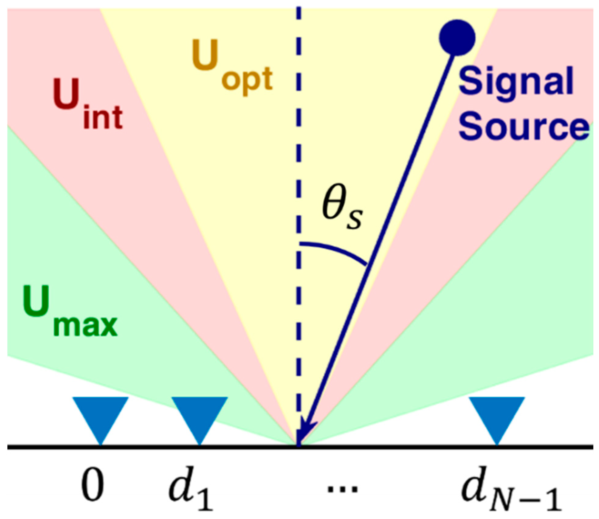
. By recalling that the array can only receive signals with DoA
in the sector
, and that the we are only interested in estimating the DoA of the sources located in the sector
, we have
and
. Hence, the difference
is bounded as
where
. For a given
, the coordinates of the endpoints
and
for the array
in the plane
can be derived by inverting Equation (12)
Given the biunivocal relationship between and , determining whether an array configuration is admissible or not is now straightforward. Specifically, an array can be considered admissible only if the corresponding segment in the plane does not intersect the contour for any . This condition guarantees that the sidelobes of the array beampattern are lower than , which in turn allows for satisfying the constraint on the maximum pairwise error probability. The following example allows for the visualization of the relationship between and , and further clarifies the notion of admissibility.
Let us assume an
and a maximum acceptable pairwise probability
. By inverting Equation (9), we obtain
. The corresponding contour plot of the
function is represented in
Figure 4a. As is apparent, the region external to the contour lines, namely the green area, represents the set of
values that satisfy the constraint
.
Now, consider the following array configurations, characterized by
:
As explained previously, these array configurations can be represented in the plane
as segments lying on the line
, and the extrema of these segments depend on the value of
. Assuming
(i.e.,
), we evaluate the endpoints
and
through Equation (17), and we represent the four considered configurations in
Figure 4a as colored segments
to verify their admissibility.
As visible in
Figure 4b, for
configurations
and
are admissible, since the segments representing their beampatterns do not intersect any replica of the likelihood function (except for the replica
, which is the likelihood function main lobe). Conversely, configurations
and
are not admissible, since the segments representing their beampatterns do intersect the contour
for
and for
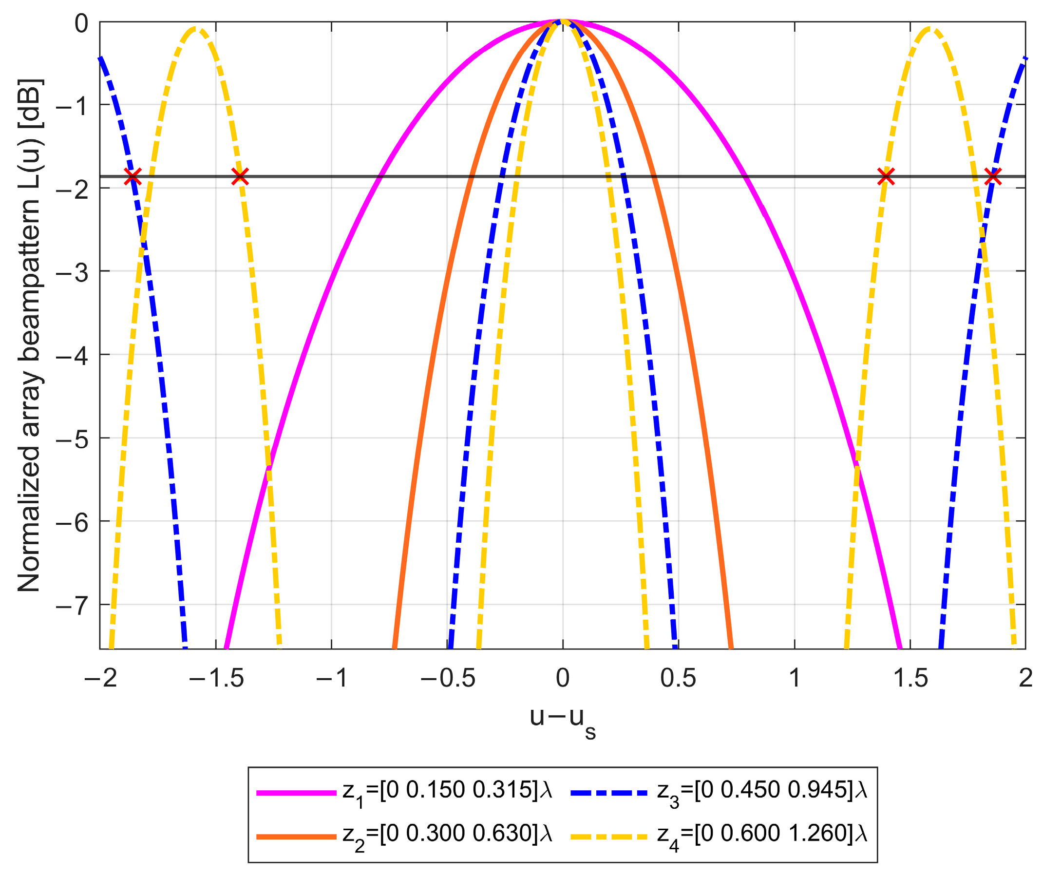
. The four array beampatterns are also represented in
Figure 5 as a function of
. Comparing these beampatterns, we notice that the array configurations denoted as
and
achieve the lowest sidelobes, while the others have high sidelobes that prevent fulfilling the requirement on
.
Notice how the beampatterns of the array configurations characterized by the same value are merely stretched versions of the same likelihood function. Specifically, the slope defines the shape of the likelihood function, while the value determines the abscissa of the axis in which the likelihood function is cut to obtain the array beampattern.
As mentioned in
Section 1, a straightforward approach to measure the robustness of a given array configuration to estimation ambiguities was proposed in [
31], based on the maximum admissible phase error. Therein, the authors introduced the synthetic parameter
, defined as the minimum distance between the folded replicas of the line
, with the wrapped phase within the angular sector
. The minimum distance
) of an array provides its maximum admissible phase error and is therefore a measure of the array’s immunity to ambiguities. By assigning a minimum acceptable distance, the parameter
can be used to determine the admissibility of an array.
The approach in [
31] is inherently different from the one proposed in this work, since it capitalizes on the phase ambiguity of the involved baselines rather than on the statistical formulation of the MLE. However, the two approaches generally provide consistent results. To carry out a comparison, we used the algorithm described in [
31] to evaluate
for the array configurations in
Figure 4a, with size scaled by
and reported their values, together with the corresponding maximum pairwise error probability
.
As visible in
Table 1, requiring that
is equivalent to requiring that
. However, while
ranges from
to
taking several intermediate values for different array configurations,
only takes two values, namely
for more robust configurations, and
for less robust examples. This suggests that constraining
provides an approximate admissibility criterion, while the proposed approach enables a more accurate assessment of array robustness to outliers. As a consequence, the two approaches provide consistent results for all array configurations, showing a well-defined behavior with respect to the presence of outliers. In contrast, they might yield conflicting indications for edge case configurations.
For example, from
Table 1, we notice that the constraint
is almost equivalent to the constraint
. With these parameters, the two approaches agree on the admissibility of both configurations
and
for any
value. However, when
, the criterion
suggests that all the included array configurations should be considered admissible. Conversely, we notice that configuration
z4 does not satisfy the constraint
, being characterized by
, and thus it would be discarded using the proposed approach. Similar considerations apply to configuration
when
.
Clearly, different values of and can lead to different edge cases on these arrays. Furthermore, additional edge cases can be found, considering array configurations with different slopes . However, the example above shows that the ML-derived proposed approach enables a more precise assessment of the array robustness to outliers, allowing us to better identify the boundaries of the APP region where the best constrained configurations in terms of MSE typically lie. This is shown in the following.
The green region in
Figure 4b identifies the subset of abscissa values
, for which a cut of the likelihood function provides an admissible array beampattern, namely
such that
. The extrema of the green patch are denoted as
. This abscissa value defines the longest admissible array with
, so that every array configuration
such that
is admissible.
Notice that the value of depends on the chosen slope . Hence, if we determine the value of maximum abscissa for every possible slope , we can identify the region in the plane which contains every array configuration that satisfies , namely the APP region.
In principle, the value can be derived as the intersection between the contours and a line through the origin with slope . Thus, the APP region can be derived in the plane before setting a specific value for .
Once the APP region has been identified, the value of is required to relate the coordinates to the inter-element distances . In other words, as visible from Equation (17), the definition of the endpoints of the segment associated to an array requires both the knowledge of and of . Therefore, the admissibility of a specific array depends not only on the constraint on the pairwise error probability, but also on how the sectors and are chosen.
For every slope , the analytical value of the optimal can be identified as follows. First, we notice that is symmetrical with respect to the two bisectors of the first and the second quadrants of the plane .
By defining the new set of coordinates
and
, such that:
and applying the transformation, we obtain
which can be easily solved for
, obtaining:
Using Equation (21) in Equation (19) allows us to express the points on the contour of
defined by
, in terms of
, as:
Since the segment representing an array lies on a line through the origin, the slope of the line crossing the contour of the replica
is given by the ratio
where
refers to the slope obtained from the positive solutions, and
refers to the slope obtained from the negative ones. As
varies in the range
, the results in Equation (23) provide the slopes of the lines crossing the replica
of the contour
and allow us to identify the maximum and minimum slope of its crossing line
By exploiting the previous analytical re41sults, together with the observation that the lower order replicas block the limiting effect of the higher order replicas, we propose the following procedure to identify the APP region in the plane. First, we identify the relative to the slopes crossing the lowest order replica, then we progressively evaluate the relative to the slopes crossing higher order replicas, until all slopes have been assigned a value , since by construction , in the following, we only consider . The following procedure is obtained:
Inside the set of all possible slopes , determine for the subset of slopes blocked by the first-order replica of the function, i.e., . Notice that all the replicas are blocked by replica (0,1) so they will be ignored in the following.
Determine the set of the non-blocked slopes after step I.
Determine for the subset of slopes blocked by next higher-order replica of the function, i.e., . Notice that the replicas are blocked by replica (1,1) so they will be ignored in the following.
Determine the set of the non-blocked slopes after step III.
Determine the subset of slopes blocked by next higher-order replica of the function.
Determine the set of the non-blocked slopes after step V.
Repeat steps V and VI until the set of non-blocked slopes is empty.
Conceptually, the presented procedure could be extended to N = 4 antenna elements, by operating in a 3D space, where the contours are replaced by surfaces, and the APP region resembles a Swiss cheese block. While the extension is straightforward, the analytical derivation would make the description uselessly cumbersome. Therefore, we avoid an explicit illustration of this case and leave it to the purview of interested reader.
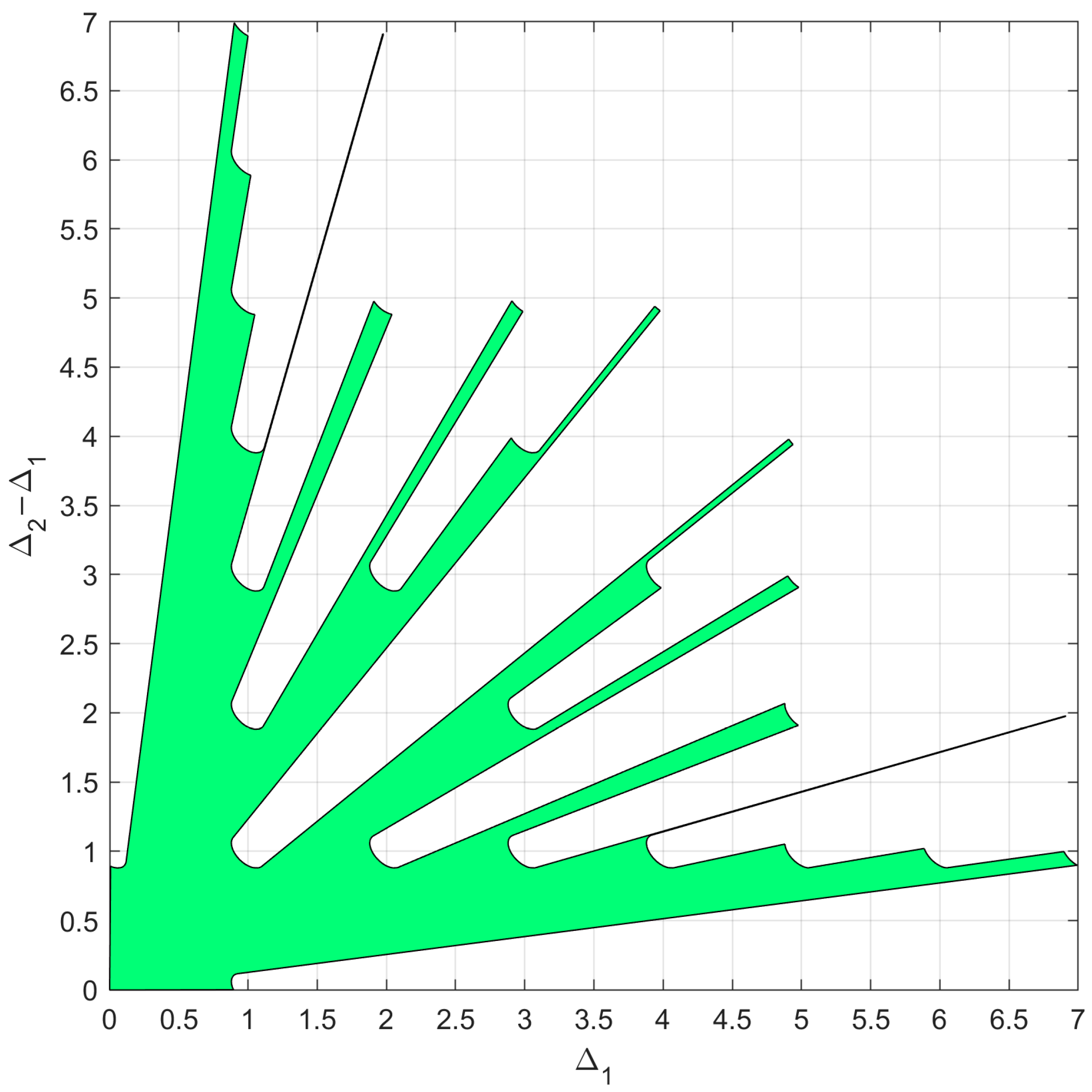
As an example of the application of the
case, the proposed procedure is applied for the case with
and
, resulting in
. Since only slopes
are of interest, the APP region occupies only the portion above the bisector of the first and third quadrant of the plane
as shown in
Figure 6, after remapping in the plane
.
Notice that the above procedure allowed us to determine the APP region in the plane . By defining the extrema and of the angular sectors and , we can map the admissible region in the plane of the array parameters . The identified APP region will be the basis for the array design approach presented in the following section.
4. Three-Element NULA Design Strategy
In this section, we present the design strategy for the three-elements array aimed at low-cost low-weight sensors for DoA estimation. Based on the MSE approximation in Equation (7), it is clear that minimizing the does not guarantee the best performance outside the asymptotic region, since for limited , there might be a significant error contribution caused by the outliers that tend to concentrate around the DoAs, , where the beampattern exhibits its peaks. Moreover, Equation (7) shows that the values of act as scaling factors for the large error contributions that add to the .
Therefore, for a given
, the only configurations that are of potential interest (i.e., provide small MSE) all have
values below the maximum acceptable value,
Pmax, and belong to the APP region. The procedure presented in
Section 3 is therefore a useful tool to restrict the search for valuable array configurations and is used as an important part of the proposed design approach.
Inside the APP region, the optimum array configuration
is obtained, adopting a minimax criterion as the one that minimizes the maximum MSE over any desired range of source angles,
:
can be either coincident with the whole sector of sources of interest
(i.e.,
), or it can be a smaller sector, where a higher accuracy is desired (i.e.,
). This formulation is equivalent to:
Since this array optimization approach is based on achieving the minimum MSE while keeping the probability of outliers under control, the obtained solution is referred to as the best outlier controlled array (BOCA). Its implementation diagram is sketched in
Figure 7. The four blocks perform the following steps:
- (i)
Identify the APP region in the plane
, using the procedure in
Section 3;
- (ii)
Set the value of , the maximum value for , based on the sensor estimation characteristic and operational scenario;
- (iii)
Map the APP region into the plane, based on the value of ;
- (iv)
Look for the array configuration providing the minimum of the MSE inside this region.
Notice that the APP region resulting from step (i) has been evaluated in the
plane. Recalling the definition of
in Equation (12), the APP region in
Figure 6 can be remapped in the
plane by scaling the maximum acceptable value
for every slope
by
. Hence, the inter-element distances
of the array configurations inside the APP region are given by
The scaling in Equation (27) requires knowledge of , which in turn requires defining the sectors and . The bounds of these sectors largely depend on the considered application and purpose, as illustrated in the following section.
Equation (27) allows us to represent the APP region in the array inter-element distances axis system, i.e., in the plane, thus fulfilling step (iii). The final optimization algorithm (step (iv)) is based on a minimax criterion by choosing the array configuration that minimizes the maximum MSE obtained inside a given angular sector .
When compared to conventional, well-known array design strategies, such as the one presented in [
28], the proposed approach offers three main advantages:
It allows for the relaxation of the half-wavelength quantization constraint on the inter-element distance.
It offers a high level of flexibility, as it allows us to distinguish the angular sector where the source can be located, the angular sector where the source is pursued, and the angular sector , where the performance is optimized.
It allows us to obtain satisfactory DoA estimation performances, even when the is in the threshold region, thanks to the constraint imposed on the maximum pairwise error probability.
In order to illustrate these advantages, in the next section, we assess the performances obtained by the BOCA in different case studies via numerical analysis.
5. Performance Assessment on Simulated Data
The purpose of this section is to test the proposed design approach against simulated data in order to prove its effectiveness. In addition, we compare it to the conventional design strategy presented in [
28], where the array inter-element distances are subject to a
quantization. To make a fair comparison, we compare the proposed BOCA with a quantized array that satisfies the same constraint on the maximum pairwise probability. This can be achieved by selecting one of the quantized array configurations falling inside the APP region, as conducted for the BOCA. The selected array will be referred to as
-best outlier controlled array (
-BOCA). Due to the quantization constraint, we expect that the
-BOCA will obtain an equal or higher MSE than the BOCA. Furthermore, there might be cases in which a
-BOCA is impossible to locate, as all quantized configurations fall outside the APP region.
As mentioned in the previous sections, the APP region depends on both and , while the selected BOCA inside the APP region changes with . Since different values for , , and can be selected based on the requirements of different applications, we define two case studies that will be used for performance assessment:
- (i)
Case A: , so that the source can be located at any possible DoA. Therefore, the possibility of having sources outside the angular sector of interest is considered.
- (ii)
Case B: , so that the possibility of having targets outside a given angular sector is excluded. This can be useful when electromagnetic shielding is employed, or when the antennas are characterized by a very directive pattern.
Both case studies are considered in
Section 5 and
Section 6, respectively dedicated to unconstrained and constrained design solutions. Notice that restricting
, as in case B, leads to smaller values of
, and thus to larger APP regions, as shown in Equation (27). In turn, this allows us to choose longer array configurations, which exhibit better performances in terms of MSE.
To study the performance of the resulting BOCA, for both Case A and Case B, we evaluate the MSE of its DoA estimate inside the area of interest (, ) as a function of the two remaining parameters, namely and , assuming assigned values for and . Since the MSE is variable in this region, a compact method to represent the performance is to average its value inside the sector . This provides us with a single averaged MSE value for each choice of and since , the angular sector in which performances are studied, is a subset of the sector of the sources of interest, i.e.,: .
To show numerical results, we assume an
value of
and we fix
.
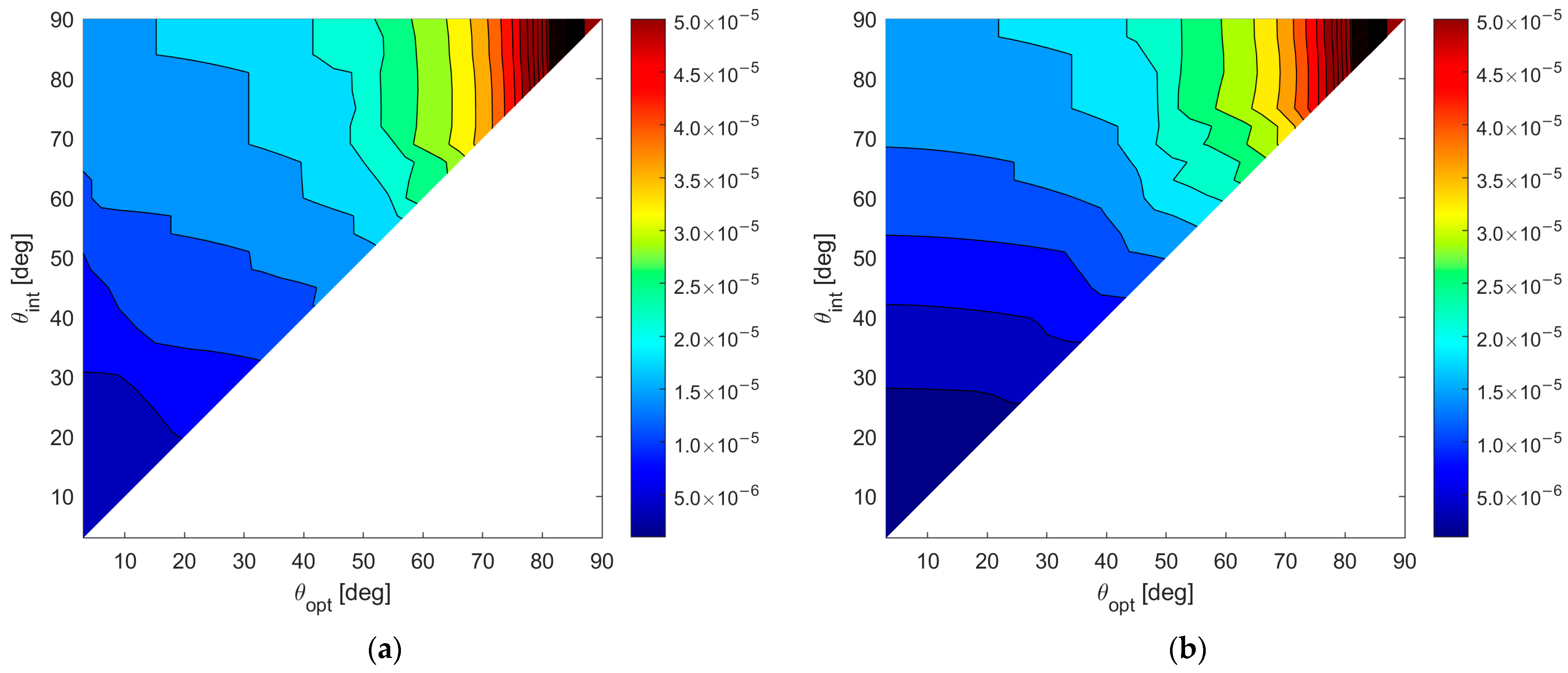
Figure 8a,b shows the map of the average MSE for case A and case B, respectively, for all the admissible values of
and
. According to these results, the following observations apply:
- (i)
Wider angular sectors result in higher values of MSE, whereas when we are interested only to the DoA estimate inside a narrow angular sector, much better MSE values can be obtained.
- (ii)
For greater values of the admissible region becomes smaller, leading to BOCA solutions with a higher MSE.
- (iii)
Hence, the larger the and are, the higher is the average MSE.
- (iv)
Case B provides generally lower values for the average MSE, since the smaller value of provides a wider APP region, thus increasing the opportunity to select a longer BOCA configuration.
To compare the performance of the BOCA and the
-BOCA, it is convenient to define the ratio
between the two mean MSEs, namely:
While the maximum (worst) MSE inside the sector
for the BOCA is always smaller compared to the
-BOCA, the ratio
of the averaged MSEs over the sector
are not necessarily greater than the unity. This ratio allows us to quantify the average improvement achieved by the proposed approach over the conventional method, as a function of
and
, over the whole area of interest.
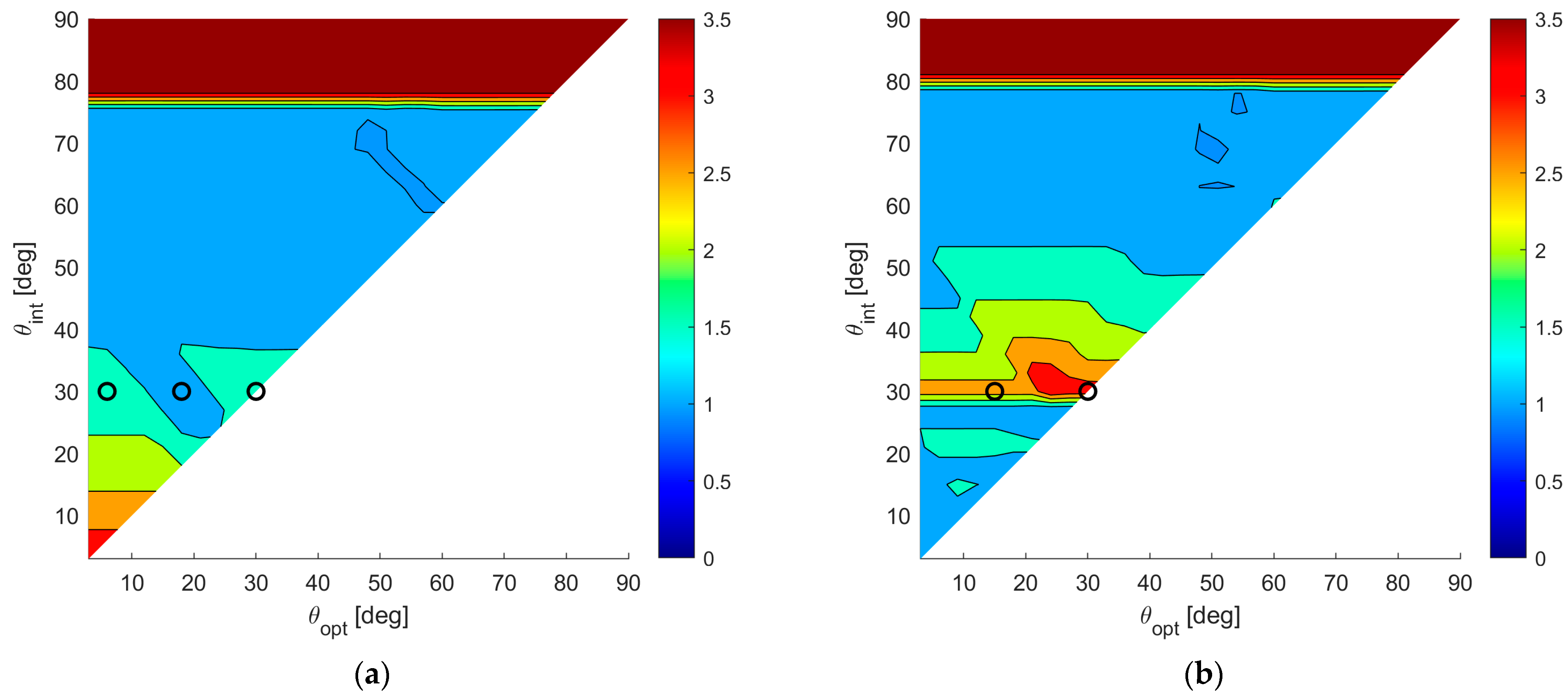
Figure 9a,b shows the
map for case study A and case study B, respectively.
By observing these results, the following remarks apply:
- (i)
The maximum achievable ratio is . This means that is at most about 3.5 times higher than ).
- (ii)
As anticipated at the beginning of this section, there are cases in which no -BOCA can be found. For the selected parameters and , this occurs when choosing . In these cases, the ratio shown in the figures has been conveniently saturated to its maximum value, namely 3.5, to denote that the improvement is not measurable.
- (iii)
As previously mentioned, in case B, we obtain wider APP regions. Therefore, longer arrays are generally admissible, and the average MSE in case B is always smaller or than or equal to the average MSE in case A, for any given pair of and .
- (iv)
Finally, while in case A, the best ratio values are obtained for smaller and , in case B, the best ratio values are obtained for .
To complete the analysis, we show the detailed performance analysis for few specific parameter sets
, corresponding to the points of the
maps in
Figure 9a,b, as shown with black circles, with the selected parameters
, and
for each case study.
5.1. Case Study A—Source Located within the Whole Angular Sector ()
In case study A, we focus on three subcases characterized by
. However, while the average MSE of both the BOCA and the
-BOCA monotonically increase with
, their ratio shows a different behavior, namely
at
and
at both
and
. As the considered subcases are characterized by the same values of
and
, they all share the same admissible region, as represented in
Figure 10.
The location of the BOCA and
-BOCA for the three subcases is represented with a blue and a green circle, respectively, in the three subplots. With the selected set of parameters, the optimization procedure leads to the BOCA and
-BOCA configurations reported in
Table 2.
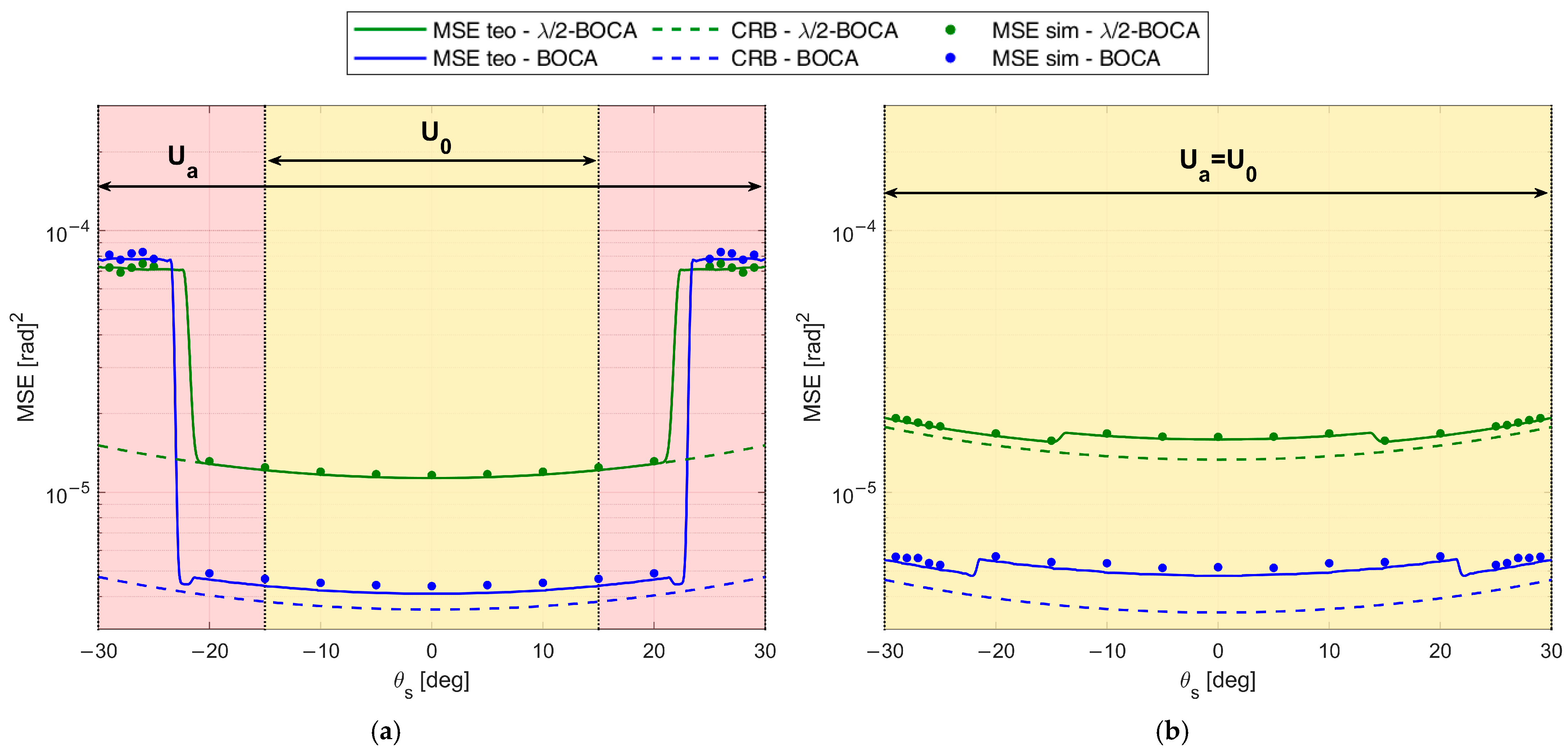
Figure 11a–c shows the MSE obtained using the
and the
, respectively, for case studies A1, A2, and A3 as a function of
. The solid curves represent the theoretical MSE, while the dashed examples represent
. Furthermore, dots represent the MSE obtained through simulation, and the vertical dash-dot lines denote the area where we look for the optimal solution.
The numerical MSE values were obtained through a Monte Carlo simulation, with runs. The simulated array output was generated according to the signal model in Equation (2), where the random samples in the noise vector were assumed to be complex valued and Gaussian distributed, namely: . The complex-valued amplitude of the source baseband signal is a deterministic parameter, set so as to guarantee the required condition, namely .
Figure 11a shows the MSE of
to be lower than those of
=
(see × markers in
Figure 10) for
; however, for
, the BOCA is subject to the presence of a sidelobe, and its MSE shows a step increase, whereas the
-BOCA is not subject to this effect. As clear from
Figure 11b, for values of
, the BOCA configuration changes to
, while the
-BOCA remains unchanged (see ○ markers in
Figure 10).
While the new BOCA still has a lower MSE than the
-BOCA, its value is not as low as it was previously. When
, the array
is subject to the presence of a sidelobe, which provides a step increase in the MSE, so that the
-BOCA configuration changes to
, as apparent from
Figure 11c. Its average MSE value increases, whereas the BOCA configuration is not subject to significant changes (see + markers in
Figure 10).
We also observe that when the MSE is too high, the simulated and theoretical MSE curves do not match exactly. This is because the union-bound approximation in Equations (7) and (8) is not tight.
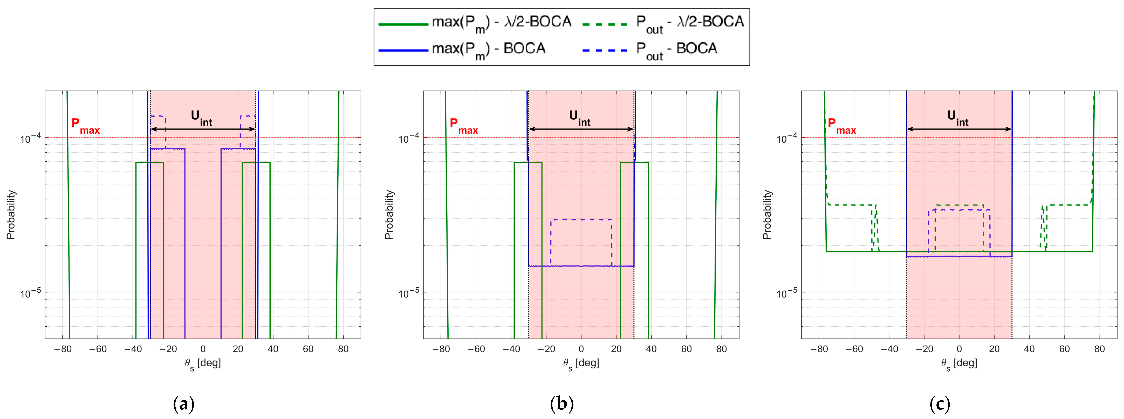
To complete the analysis,
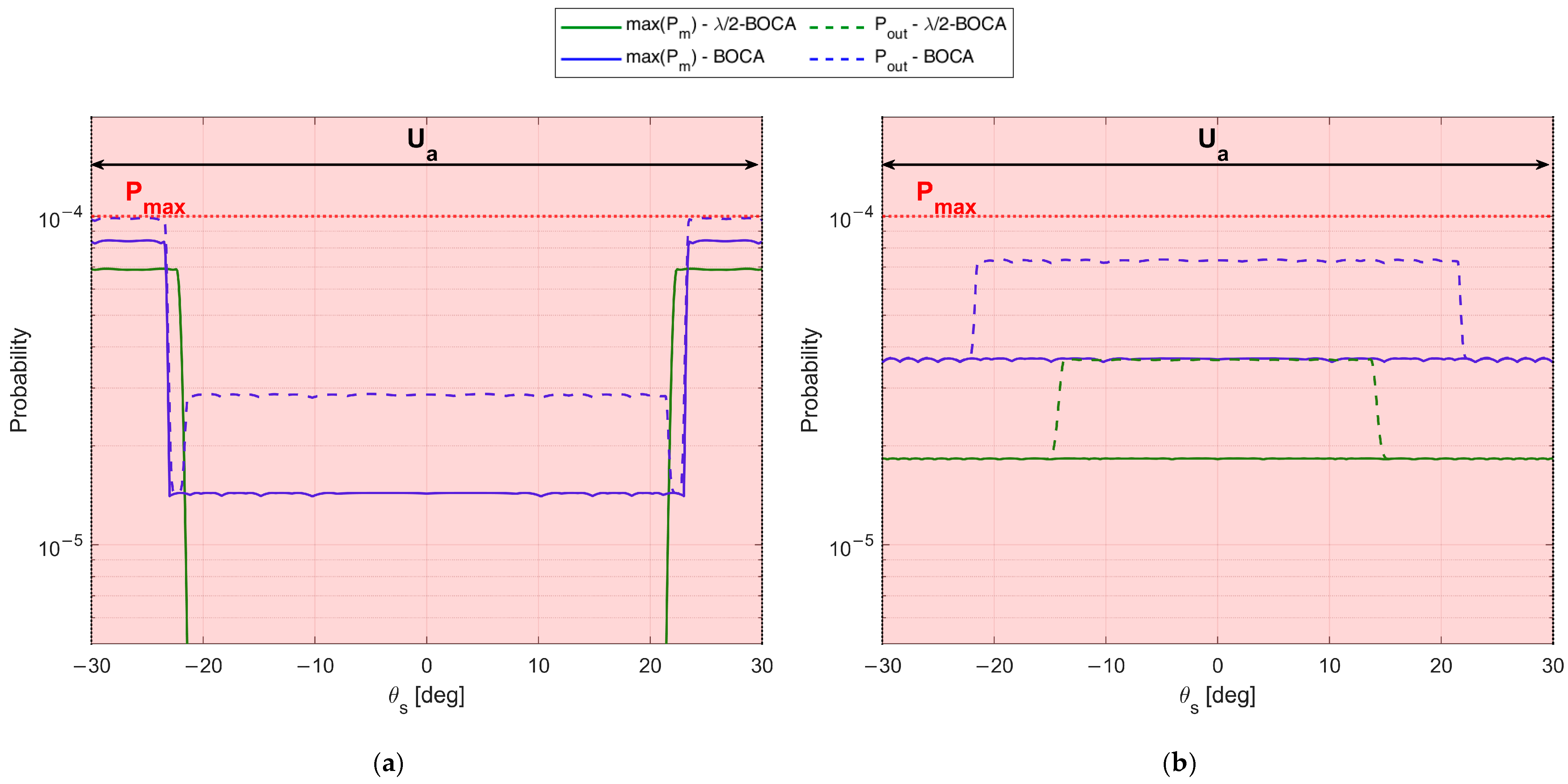
Figure 12 shows the maximum pairwise probability for each array configuration. The vertical dash-dot lines denote the area where the constraint must be guaranteed, while the horizontal dashed line represents the constraint value
.
Figure 12 illustrates that both the
-BOCA and the BOCA satisfy the constraint on the maximum pairwise probability inside the angular sector
, as we expected. However, as shown in
Figure 11, the BOCA performs better inside the
angular sector in terms of MSE.
5.2. Case Study B—Source Only Located within the Angular Sector of the DoA of Interest
As opposed to case study A, in case B, the possibility that a source might be located outside the angular sector of interest is excluded, i.e.,
. We focus on two subcases characterized by
, as they seem to be the cases in which the best ratios
are obtained. As in case A, the different subcases are characterized by the same admissible region, as represented in
Figure 13. With the selected set of parameters, the optimization procedure leads to the BOCA and
-BOCA reported in
Table 2.
Note that the decrease in
yields a larger admissible region. This allows us to choose longer array configurations, which were non-admissible in case A. Despite this, the
-BOCA is still the one selected in the previous cases, confirming the reduced flexibility of the quantized approach. These considerations are further confirmed by
Figure 14a,b and
Figure 15a,b, where the MSE and the maximum pairwise error probability obtained using the different configurations is evaluated across a grid of
values.
As a final consideration, we notice that the admissible regions shown in
Figure 10 and
Figure 13, have very spiky shapes in certain areas. Selecting an array configuration inside one of those thin portions would mean requiring an installation accuracy that would be unlikely to be guaranteed in practice. Furthermore, these types of solutions are highly unstable, and lead to the variability of the ratio
with
. Therefore, in the next section, we modify the optimization problem by adding additional constraints that might be required for the practical application of the proposed approach.
6. Constrained Three-Element NULA Design Strategy
In this section, we consider two technological constraints that are likely to arise in real case scenarios, and we introduce a slight modification in the proposed strategy that will make it suitable for practical applications.
The first technological constraint is introduced based on the following observation: the APP regions shown in the previous sections always include solutions in which the inter-element distance is very small. In practical applications, depending on the signal wavelength, the physical size of the antennas, and the coupling effects that might occur, it might not be possible to position the antenna elements at the required proximity. Therefore, we consider the possibility to exclude the solutions characterized by inter-element distances shorter than a fixed value from the admissible region.
The second technological constraint is related to installation accuracy. We define a finite installation accuracy , representing the maximum error tolerated in the installation. Specifically, a given array inside the APP region is considered admissible only if the four arrays also lie within the admissible region. This excludes all the thinner areas from the admissible region.
The block diagram in
Figure 16 illustrates the constrained optimization procedure. Clearly, for
and
, the constrained design strategy corresponds to the one in Equation (26).
To show the effect of the additional constraints on the results, let us consider a passive location system operating in the Wi-Fi band at
(
). We assume that the employed commercial antennas have a size
, constraining the minimum inter-element distance. Two different values are considered for
, namely
(micrometric positioning) and
(manual positioning).
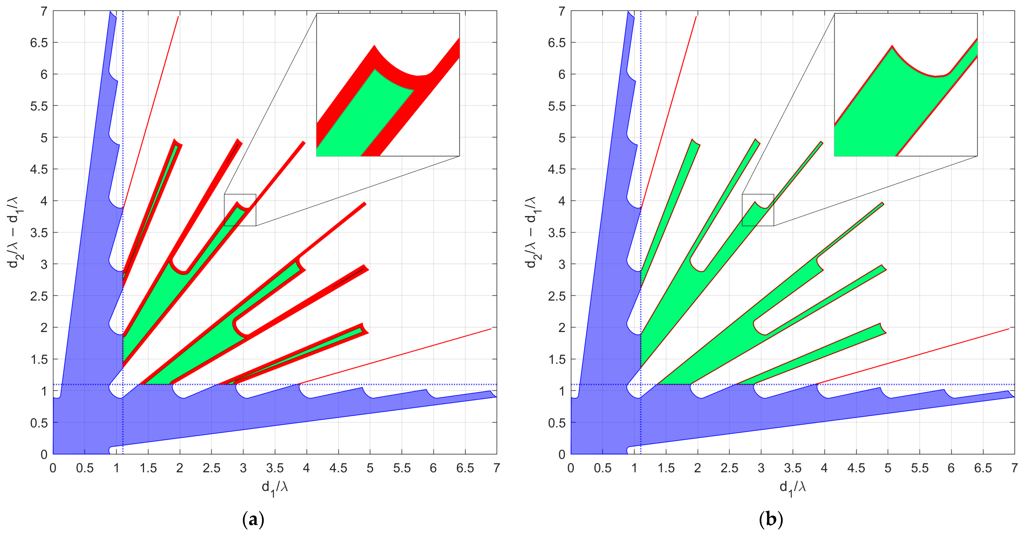
Figure 17a,b shows the admissible region obtained by including the technological constraints for the two cases, assuming
,
and
. The blue-colored areas are the portions of the APP region excluded by the constraint on the minimum inter-element distance, while the red-colored areas are the portions of the APP excluded to consider installation accuracy tolerance. As visible from
Figure 17, the installation accuracy constraint removes thinner areas from the APP region. These areas contain array configurations with highly unstable performance, for which a slight modification in the inter-element distance causes the array configuration to fall outside the APP region.
As visible in
Figure 17, the technological constraints lead to significant changes in the APP region, so that most of the array configurations considered in case studies A1-A3, and B1 and B2, are no longer admissible. Therefore, for each choice of
,
, and
, new BOCA and
-BOCA configurations must be identified. For example, considering
and
, as shown in
Figure 17b, and assuming
, the new BOCA configurations become
and
. We also notice that the obtained BOCA configuration
is characterized by a very low value of
, as evaluated following the procedure in [
31], and it would have not been considered admissible based on the maximum error criterion. However,
is guaranteed to satisfy the constraint
, since it belongs to the APP region. Therefore, in this case, the
value is not a good proxy for robustness to estimation ambiguities, since our ML-based admissibility criterion allows us to find a robust array configuration with low
. This is further confirmed by observing the ratio
between the MSEs of the
and that of the
. Since we have
, the BOCA design solution ultimately achieves an MSE which is about one-third of the MSE obtained by the
-BOCA. In conclusion,
is indeed a good alternative to both the
-BOCA and to the BOCA designs obtained in the case studies without technological constraints.
Depending on the value of the constraints and on the extrema of the considered angular sectors, the modified APP region might become so restrictive that no
-BOCA configurations could be found. In such cases, the ratio
is saturated at its maximum value, namely
.
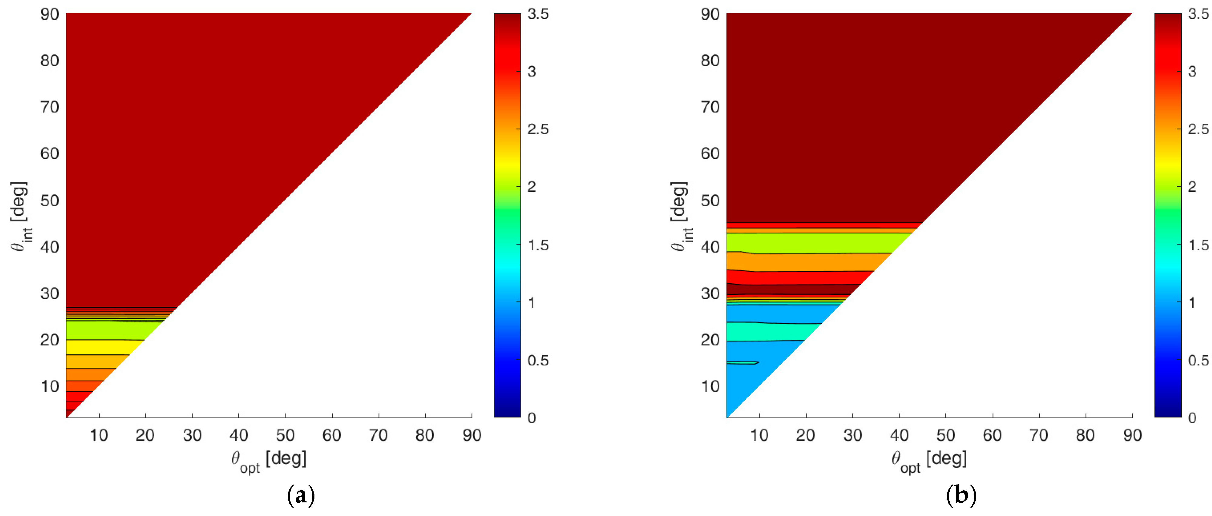
Figure 18a,b shows the contour plots of
, obtained considering case studies A and B, respectively, and assuming an installation accuracy tolerance of
. As is apparent, the additional design constraints degrade the estimation accuracies of both the
-BOCA and the BOCA configurations. Therefore, the ratio
between the two MSEs still assumes values between
and
.
By increasing the installation accuracy tolerance to
, we obtain the contour plots of
, as shown in
Figure 19a,b, relative to cases A and B, respectively.
As visible from these contour plots, the effect of the higher tolerance can provide a significant change in the array design. Specifically, most of the plane is saturated to 3.5. Based on this observation, we conclude that the proposed approach is always able to provide a valid array configuration, while there is no -BOCA solution that satisfies all the imposed constraints at the same time.
In conclusion, the results obtained in case study B, assuming are also used to validate the obtained design strategy in a real-case scenario using experimental data, as reported in the following section.
7. Experimental Results
To further support the effectiveness of the design procedure proposed in the previous sections, an experimental trial was conducted in a parking area.
For this experiment, we assumed
. The design of the array has been carried out to guarantee
when the operative
value is set to
. Finally, the minimum inter-element distance has been constrained to be
, as in the previous section, with
. With these parameters, we obtain the admissible region in
Figure 20.
To carry out the experimental acquisition, we exploited a four-channel National Instruments NI USRP-2955 board, operating in the 2.5 GHz Wi-Fi frequency band. To collect samples simultaneously with the two arrays, we must operate with two configurations that have two elements in common. For this purpose, we selected a non-optimal array, addressed in the following as Almost-BOCA array , that has one inter-element distance in common with the -BOCA, . This allowed us to make the acquisitions with a single 4-elements array with , with the individual element connected channels 0,1,2,3 of the 4-channel USRP acting as the coherent receiver. With this arrangement, the snapshots of the -BOCA array were obtained by using only the samples received by channels 0,1, and 2, whereas those of the Almost-BOCA array were obtained by using only the samples received by channels 0,1, and 3. Moreover, in this way, the snapshots of the two arrays are coherent and simultaneous. Note that the resulting array provides only slightly degraded performance with respect to the BOCA.
Figure 21a shows a sketch of the acquisition geometry. The green markers represent the element of the
-BOCA, while the blue markers indicate the elements of the Almost-BOCA. The two sensors in the middle are common between the two arrays. The four-element array that includes both the Almost-BOCA and the
-BOCA solutions was realized by deploying four Wi-Fi antennas on a plastic support mounted on a tripod.
Figure 21b shows this receiving system set in the origin of the reference system. The Wi-Fi access point (AP) in
Figure 21c is used as the transmitting source, which has been initially placed at 20 m with DoA
from the receiving antennas and then moved to
with respect to the boresight of the array. This was set to transmit the Wi-Fi beacons with a beacon interval of 3ms at
, (namely, using wavelength
).
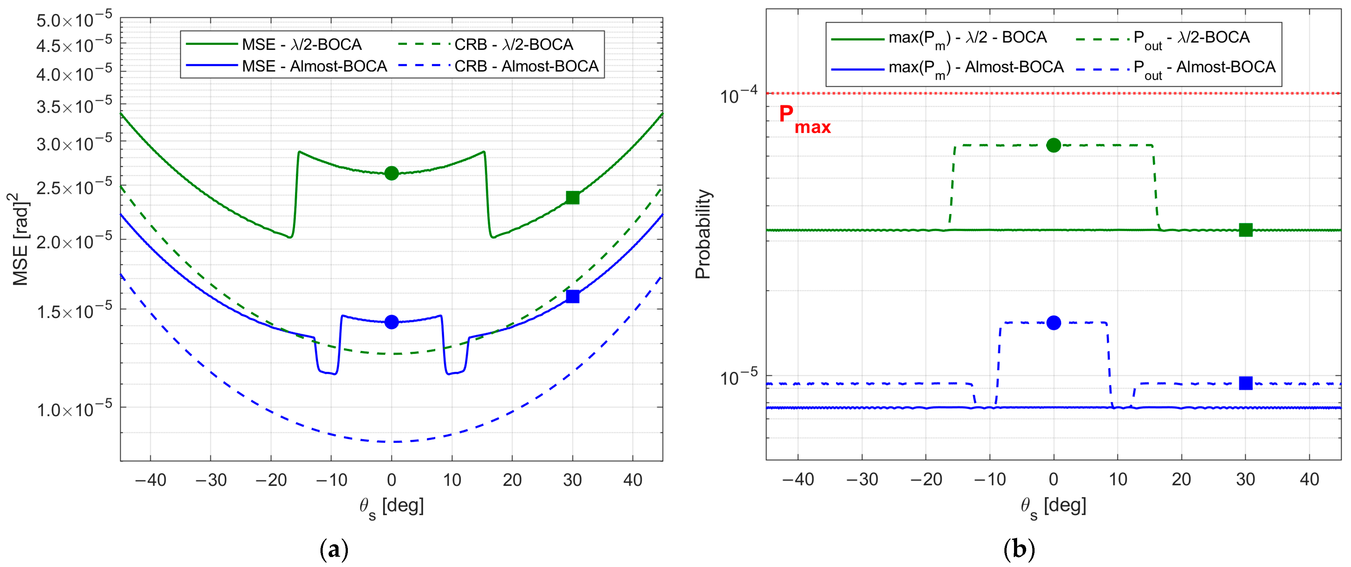
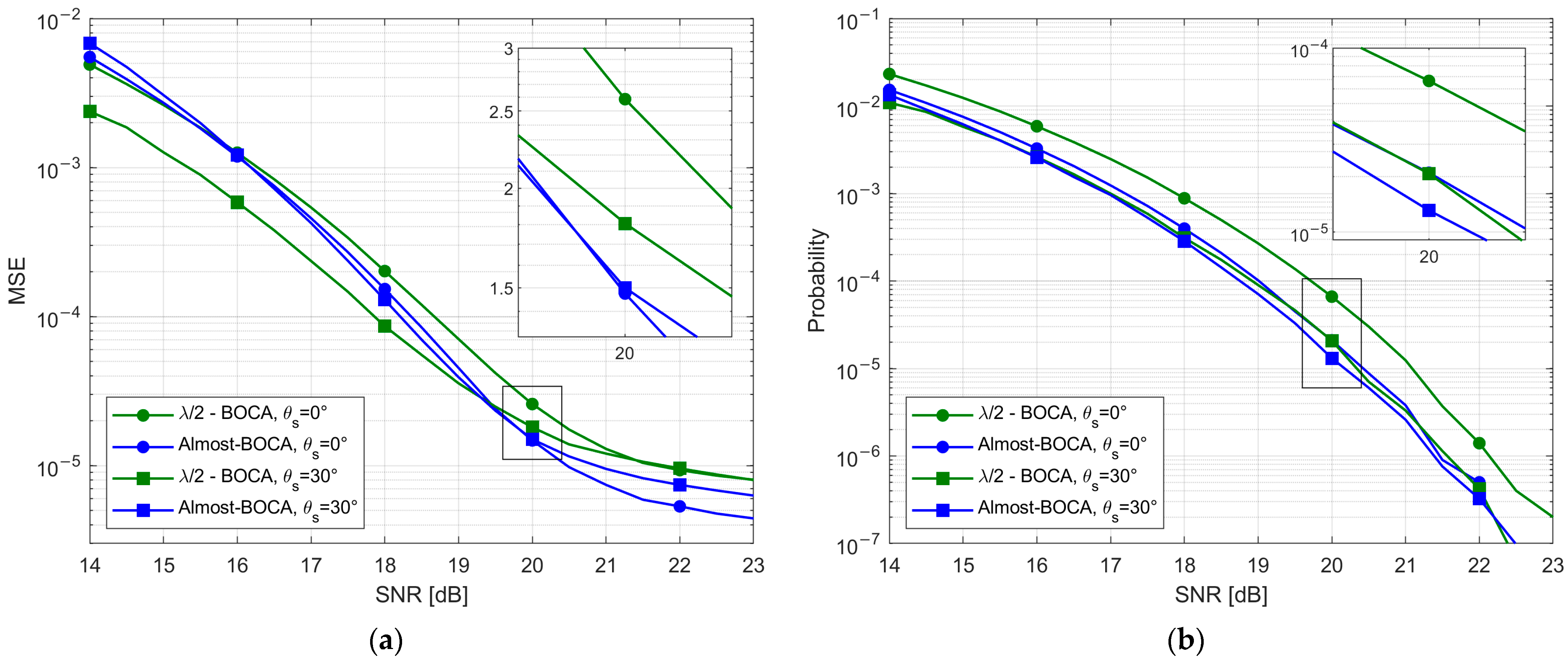
The expected performance for
in terms of both MSE and
is reported in
Figure 22a,b, as obtained from the theoretical framework in Equations (7)–(9) for both the Almost-BOCA and the
-BOCA. The following remarks apply:
When the source is located at , the MSE obtained with the -BOCA should be about times higher than the MSE obtained with the Almost-BOCA, while the is about times lower.
When the source is located at , the MSE obtained with the -BOCA should be about times higher than the MSE obtained with the Almost-BOCA, while the is about times lower.
The experimental results have been obtained by simultaneously collecting long sequences of samples with the 4 elements when the AP is active. These data are received with a measured . White Gaussian noise was added to the data to emulate lower values, specifically between and with a step.
By averaging the received samples, the resulting MSE and
curves are obtained and reported in
Figure 23a,b, respectively, as a function of the
value and for both considered DoAs. By observing
Figure 23, we note that:
For both the considered DoAs, the Almost-BOCA solution outperforms the -BOCA in the asymptotic region, since a longer array is used;
For , the Almost-BOCA solution outperforms the -BOCA, both in terms of MSE and for ;
For , the improvement is lower as predicted by theory, and starts at a higher ().
As apparent, the experimental results show that the non--spaced array always outperforms its counterpart for the design value and for higher SNR values. This confirms that the design procedure effectively allows us to design an array that provides a better performance than the -BOCA in a realistic experimental scenario.
We recall that a slightly different and better performing BOCA solution would be selected if we did not force it to have one inter-element distance in common with the -BOCA. Therefore, higher improvements are expected if the design strategy is applied with its entire set of degrees of freedom.
8. Conclusions
DoA estimation of narrowband signals is a ubiquitous task in several civil surveillance applications, such as passive coherent location systems, passive sonar, or passive radar. The main challenge in these applications is to comply with the typical low-cost requirements involving not only the economic cost, but also the computational load. Additionally, the DoA estimation accuracy is usually degraded by the presence of outliers, which occur as a result of the poor conditions characterizing low-cost systems. To achieve the required features of limited complexity and system lightness, the number of antenna elements must be kept sufficiently low. With this perspective, NULA configurations represent a viable solution to reduce the number of receiving elements without compromising performance.
The design strategy presented in this paper is set within the context of low-cost sensors applications, as it allows us to identify the so-called best outlier-controlled NULA configuration, achieving satisfactory DoA estimation performance by exploiting just three antenna elements. As a matter of fact, the BOCA solution allows for minimizing the MSE, while keeping the outlier probability under reasonable control.
The design procedure is based on the following two steps. First, an admissible pairwise probability region is identified, exploiting the algorithm presented in
Section 3. The APP region contains all the arrays for which the outlier probability is kept under control. Second, the BOCA configuration achieving the minimum MSE is located inside the APP region. It has also been shown that the APP region can be easily modified to incorporate practical design constraints, such as the minimum inter-element distance and the installation accuracy tolerance.
The proposed design strategy has been compared to the one presented in [
28], which represents our benchmark. Therein, the array inter-element distances are quantized to half-wavelength. To carry out a fair analysis, we compared the estimation accuracy achieved by the BOCA with the one achieved by the best outlier-controlled array with the half-wavelength quantization constraint, namely the
-BOCA. As shown via both theoretical and numerical analyses, the BOCA solutions generally achieve improved estimation accuracies compared to the
-BOCA estimations, with an improvement depending on how the angular sectors
,
, and
are chosen. The effectiveness of the proposed design procedure has also been verified using experimental data, confirming that the optimized array outperforms the
-quantized benchmark array. The comparison with a recent three-element NULA design approach to control ambiguity outliers is also included, which emphasizes the capability of our proposed model to accurately characterize and control the probability of ambiguities.
As a future research scope, it might be interesting to extend the design strategy to four-element and five-element NULA configurations in order to improve the estimation accuracy without significantly increasing the number of receiving channels. In such cases, alternative design strategies, such as nested or coprime array configurations, may also provide a useful benchmark. Furthermore, non-linear array configurations, such as circular arrays, could be investigated, as they would allow us to estimate the DoA regarding both azimuth and elevation. Lastly, the DoA estimation problem could be extended to multi-source scenarios, which would be useful not only when multiple sources of interest are present, but also to take any multipath effect into proper account.
