
Plant Disease Detection and Classification: A Systematic Literature Review

 ,
,  , and
, and
Abstract
1. Introduction
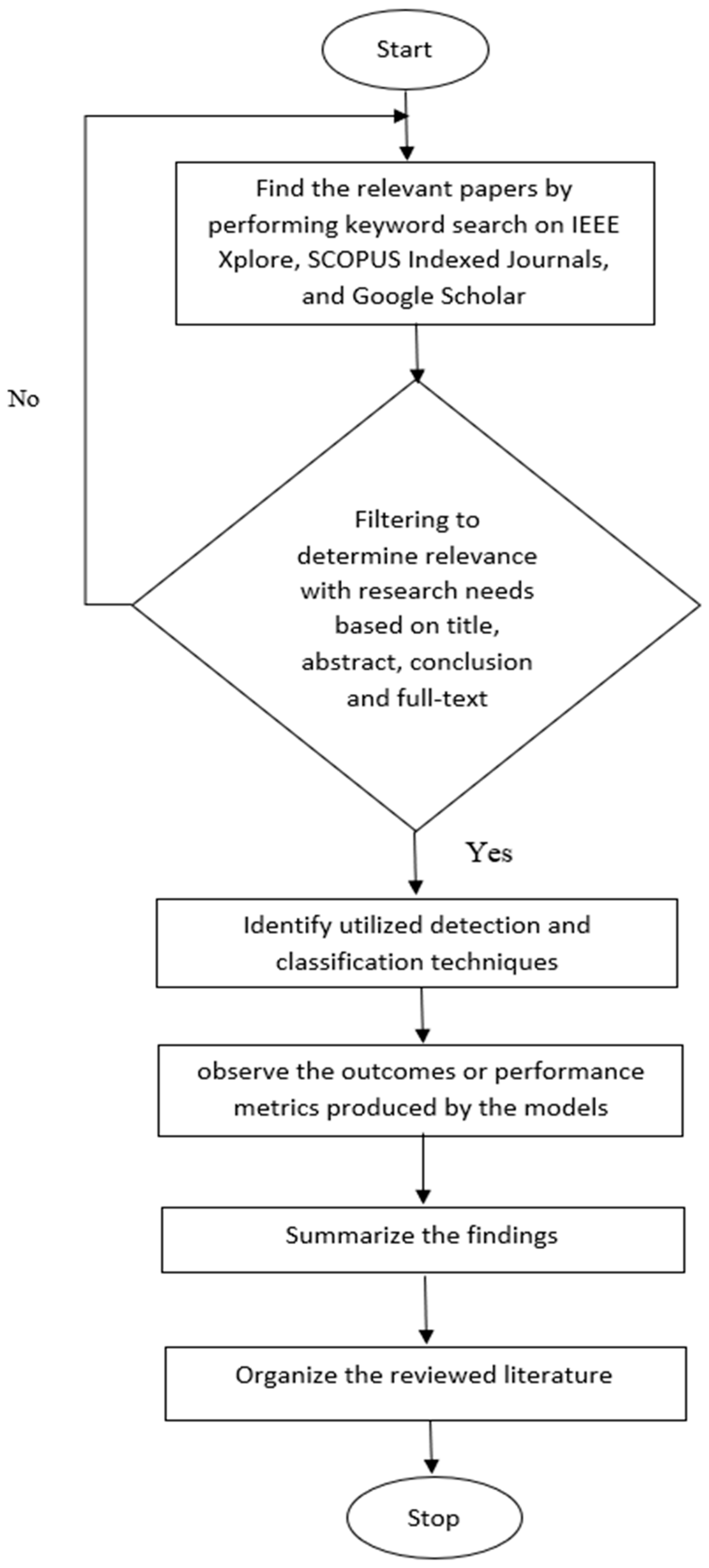
2. Methodology
2.1. Planning
2.2. Conduction
3. Related Work
3.1. Discussion for RQ1: What Are the Main Sources for Collecting Data on Plants?
Observation 1
3.2. Discussion for RQ2: What Different Pre-Processing Techniques Are Applied?
Observation 2
3.3. Discussion for RQ3: What Different Techniques Are Used for Data Augmentation?
Observation 3
3.4. Discussion for RQ4: What Kinds of Feature Extraction Methods Are Employed?
Observation 4
3.5. Discussion for RQ5: What Are the Typical Attributes That Are Used or Extracted?
Observation 5
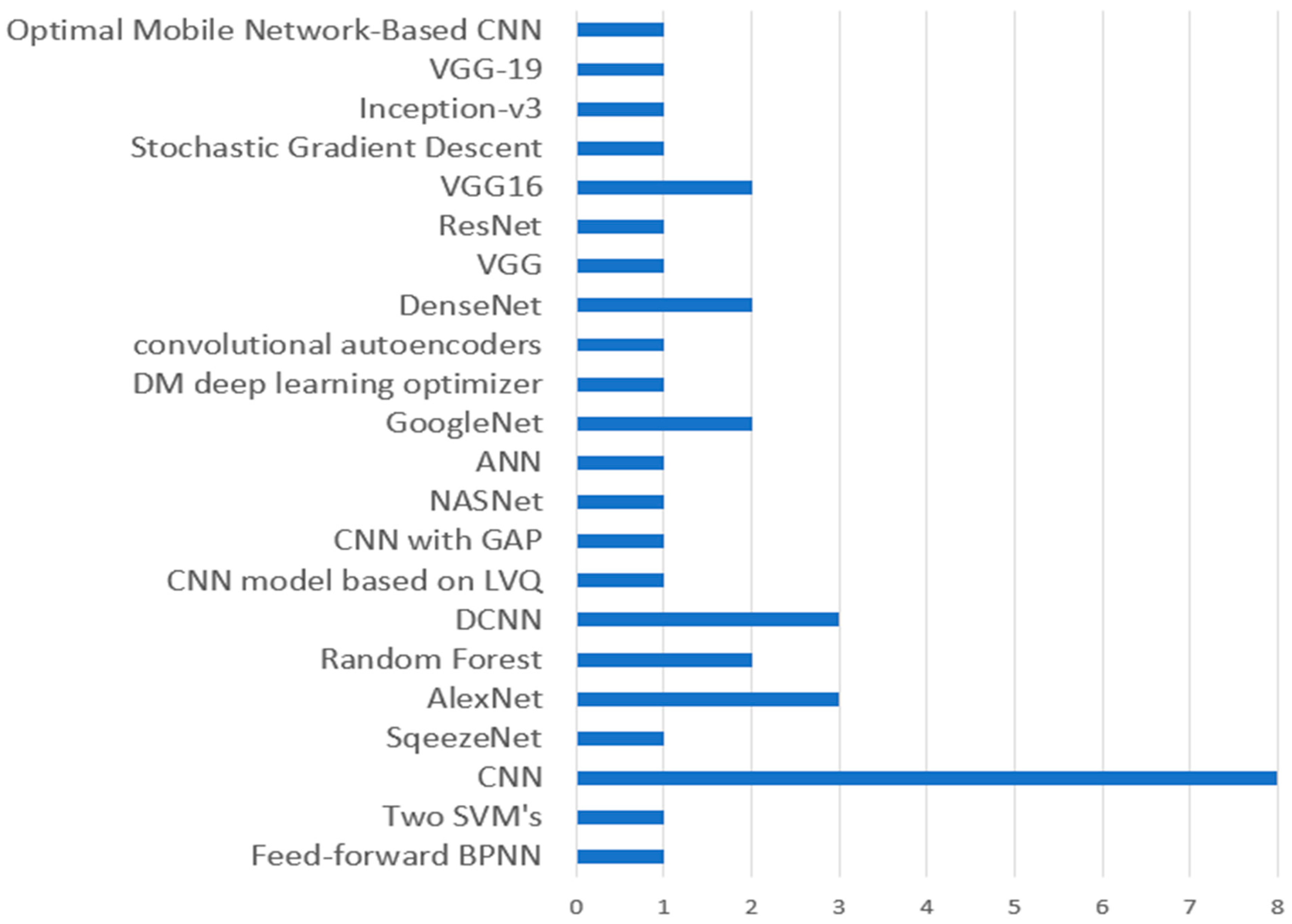
3.6. Discussion for RQ6: What Automated Systems Have Been Implemented for Identifying and Categorizing Plant Diseases?
Observation 6
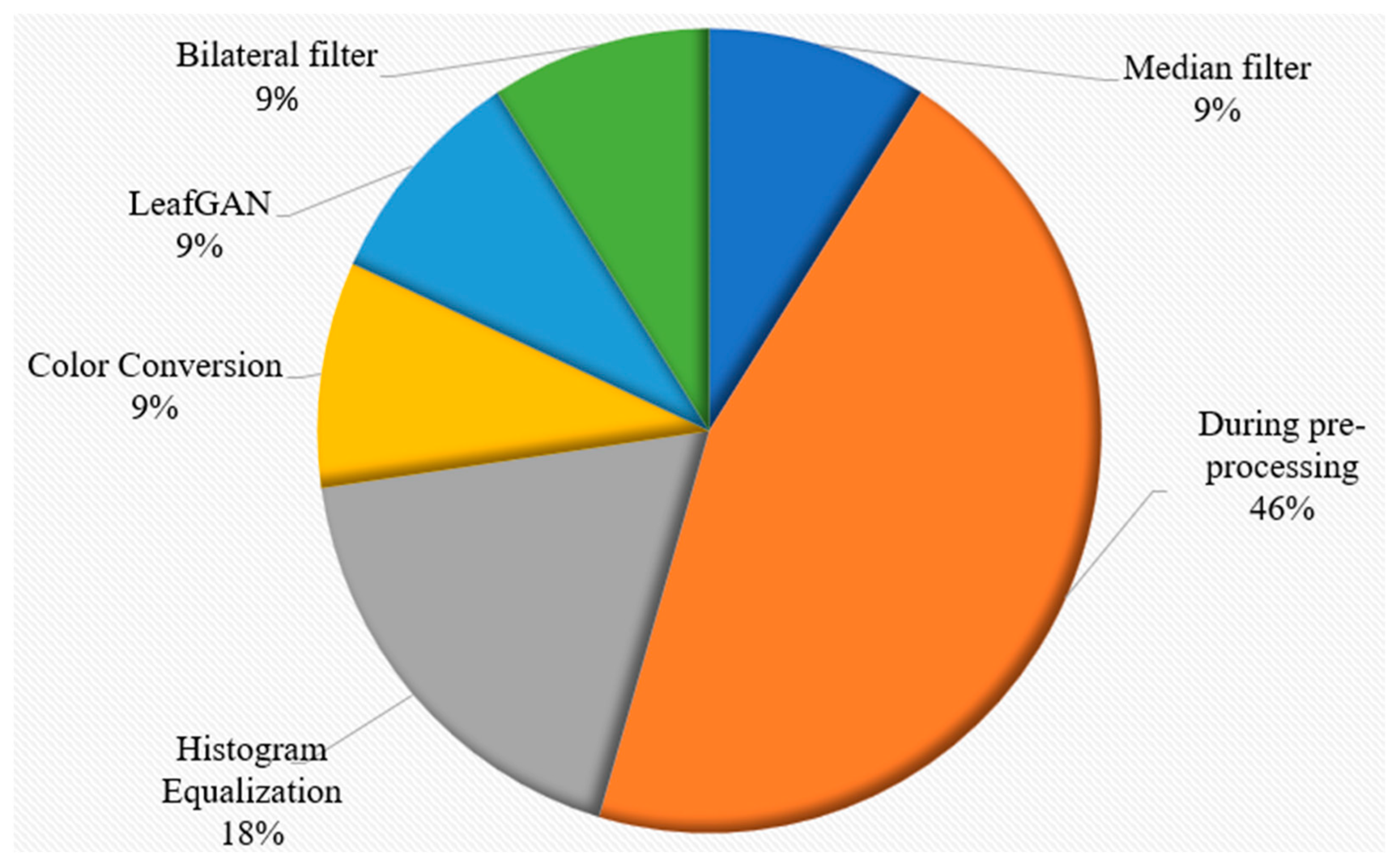
3.7. Discussion for RQ7: What Analytical Techniques Are Employed for Improving Image Quality?
Observation 7
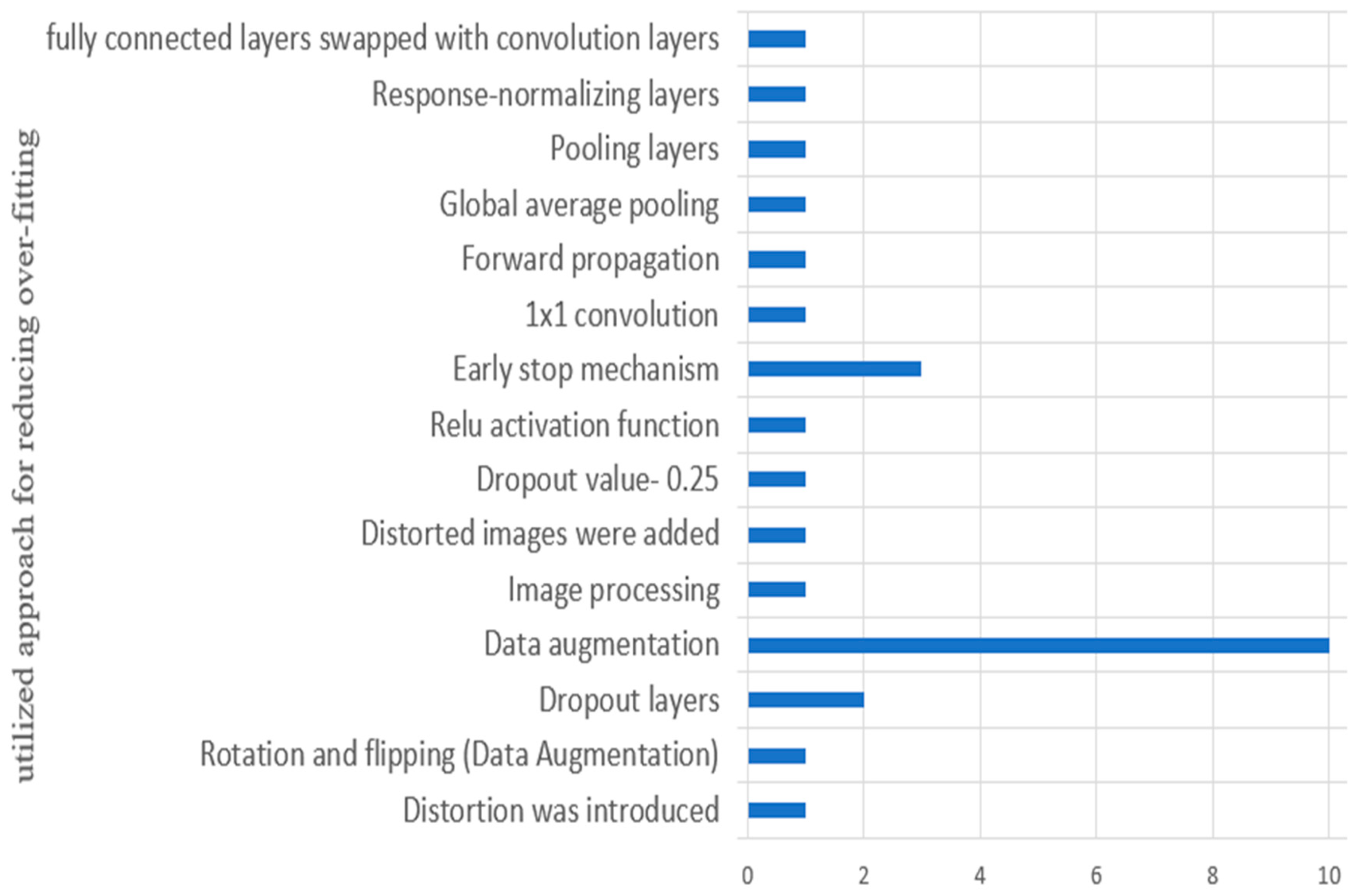
3.8. Discussion for RQ8: What Are the Techniques Utilized for Reducing/Removing Overfitting?
Observation 8
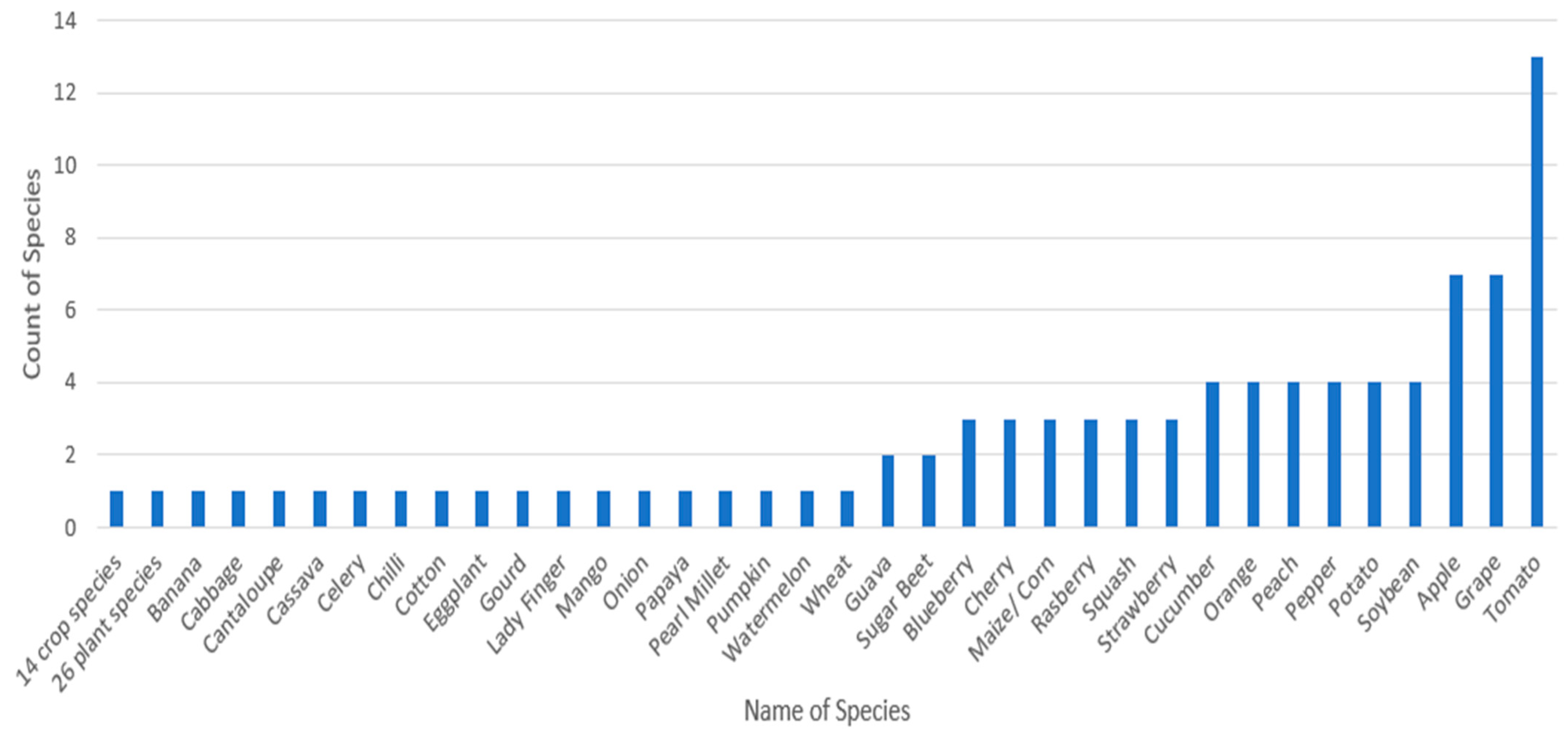
3.9. Discussion for RQ9: What Are the Different Plant Species That the Evaluated Research Is Based on, and What Classes of Diseases Have Been Found by the Evaluated Studies?
Observation 9
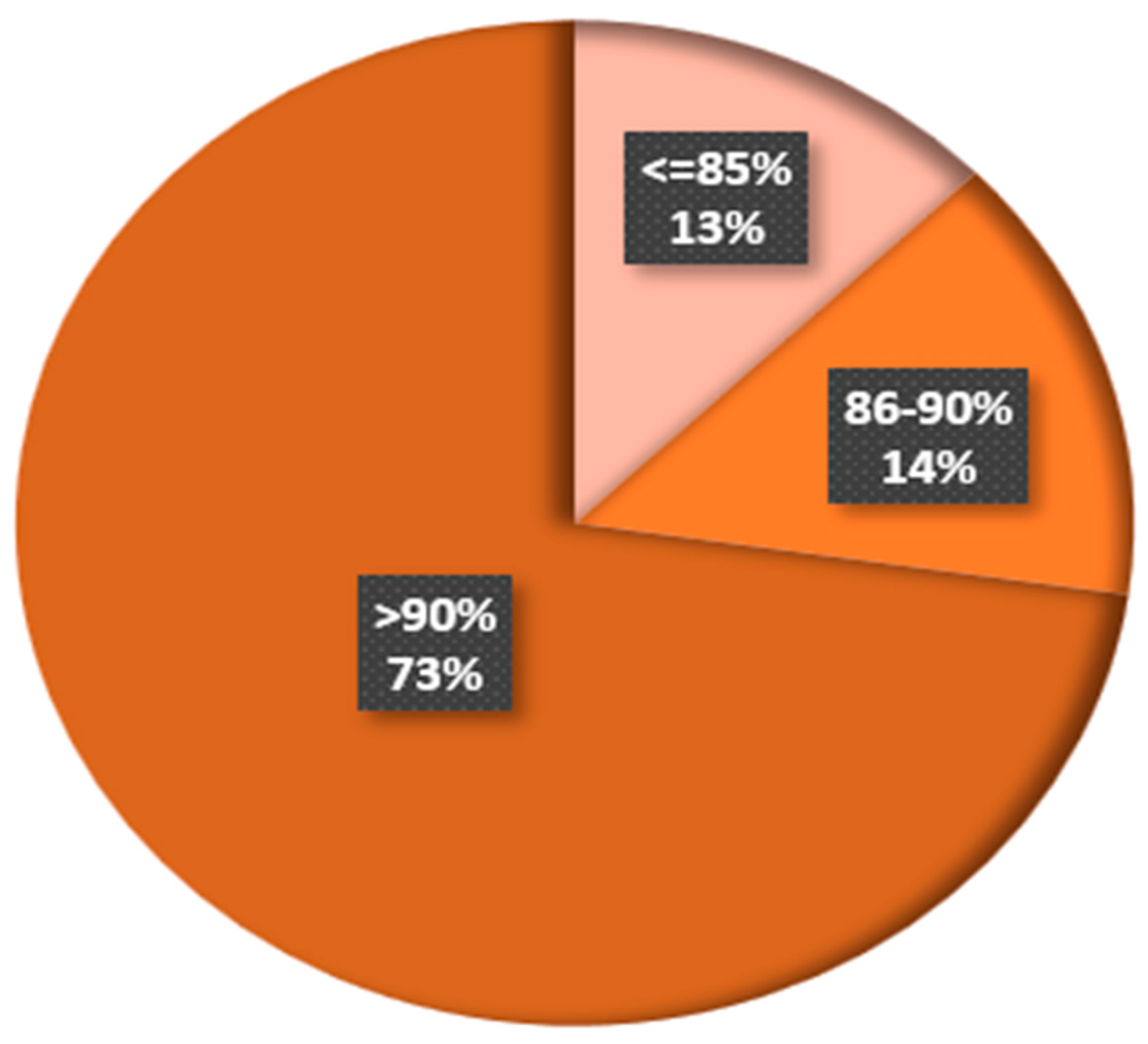
3.10. Discussion for RQ10: What Is the Accuracy of Existing Plant Disease Detection and Classification Approaches?
Observation 10
4. Challenges in Existing Approaches
- The analysis of disease classification can be impacted by environmental factors such as temperature and humidity;
- It is difficult to identify appropriate and unhealthy portions of leaves because disease symptoms are not well defined;
- Some models were unable to identify a certain stage of a plant leaf disease;
- Some models failed to extract the desired impacted area from images with intricate backgrounds;
- Several of the methods discussed in this review study were trained using the publicly available PlantVillage dataset, but they fell short when put to the test against a real-world environment.
5. Overall Observation and Comparison
5.1. Overall Observation
5.2. Comparison
6. Conclusions and Future Scope
Author Contributions
Funding
Institutional Review Board Statement
Informed Consent Statement
Data Availability Statement
Acknowledgments
Conflicts of Interest
References
- Malathy, S.; Karthiga, R.; Swetha, K.; Preethi, G. Disease Detection in Fruits Using Image Processing. In Proceedings of the 2021 6th International Conference on Inventive Computation Technologies (ICICT), Coimbatore, India, 20–22 January 2021; pp. 747–752. [Google Scholar] [CrossRef]
- Rumpf, T.; Mahlein, A.K.; Steiner, U.; Oerke, E.C.; Dehne, H.W.; Plümer, L. Early detection and classification of plant diseases with Support Vector Machines based on hyperspectral reflectance. Comput. Electron. Agric. 2010, 74, 91–99. [Google Scholar] [CrossRef]
- Dubey, S.R.; Jalal, A.S. Detection and Classification of Apple Fruit Diseases Using Complete Local Binary Patterns. In Proceedings of the 2012 3rd International Conference on Computer and Communication Technology, Allahabad, India, 23–25 November 2012; pp. 346–351. [Google Scholar] [CrossRef]
- Ramesh, S.; Hebbar, R.; Niveditha, M.; Pooja, R.; Shashank, N.; Vinod, P.V. Plant Disease Detection Using Machine Learning. In Proceedings of the 2018 International Conference on Design Innovations for 3Cs Compute Communicate Control (ICDI3C), Bangalore, India, 25–28 April 2018; pp. 41–45. [Google Scholar] [CrossRef]
- Behera, S.K.; Jena, L.; Rath, A.K.; Sethy, P.K. Disease Classification and Grading of Orange Using Machine Learning and Fuzzy Logic. In Proceedings of the 2018 IEEE International Conference on Communication and Signal Processing (ICCSP), Chennai, India, 3–5 April 2018; pp. 0678–0682. [Google Scholar] [CrossRef]
- Tulshan, A.S.; Raul, N. Plant Leaf Disease Detection Using Machine Learning. In Proceedings of the 2019 10th International Conference on Computing, Communication and Networking Technologies (ICCCNT), Kanpur, India, 6–8 July 2019; pp. 1–6. [Google Scholar] [CrossRef]
- Wahab, A.H.B.A.; Zahari, R.; Lim, T.H. Detecting Diseases in Chilli Plants Using K-Means Segmented Support Vector Machine. In Proceedings of the 2019 3rd International Conference on Imaging, Signal Processing and Communication (ICISPC), Singapore, 27–29 July 2019; pp. 57–61. [Google Scholar] [CrossRef]
- Sladojevic, S.; Arsenovic, M.; Anderla, A.; Culibrk, D.; Stefanovic, D. Deep Neural Networks Based Recognition of Plant Diseases by Leaf Image Classification. Comput. Intell. Neurosci. 2016, 2016, 3289801. [Google Scholar] [CrossRef]
- Fujita, E.; Kawasaki, Y.; Uga, H.; Kagiwada, S.; Iyatomi, H. Basic Investigation on a Robust and Practical Plant Diagnostic System. In Proceedings of the 2016 15th IEEE International Conference on Machine Learning and Applications (ICMLA), Anaheim, CA, USA, 18–20 December 2016; pp. 989–992. [Google Scholar] [CrossRef]
- Brahimi, M.; Boukhalfa, K.; Moussaoui, A. Deep Learning for Tomato Diseases: Classification and Symptoms Visualization. Appl. Artif. Intell. 2017, 31, 299–315. [Google Scholar] [CrossRef]
- Fuentes, A.; Yoon, S.; Kim, S.C.; Park, D.S. A robust deep-learning-based detector for real-time tomato plant diseases and pests recognition. Sensors 2017, 17, 2022. [Google Scholar] [CrossRef]
- Cap, H.Q.; Suwa, K.; Fujita, E.; Kagiwada, S.; Uga, H.; Iyatomi, H. A Deep Learning Approach for On-Site Plant Leaf Detection. In Proceedings of the 2018 IEEE 14th International Colloquium on Signal Processing & Its Applications (CSPA), Penang, Malaysia, 9–10 March 2018; pp. 118–122. [Google Scholar] [CrossRef]
- Ma, J.; Du, K.; Zheng, F.; Zhang, L.; Gong, Z.; Sun, Z. A recognition method for cucumber diseases using leaf symptom images based on deep convolutional neural network. Comput. Electron. Agric. 2018, 154, 18–24. [Google Scholar] [CrossRef]
- Sardogan, M.; Tuncer, A.; Ozen, Y. Plant Leaf Disease Detection and Classification Based on CNN with LVQ Algorithm. In Proceedings of the 2018 3rd International Conference on Computer Science and Engineering (UBMK), Sarajevo, Bosnia and Herzegovina, 20–23 September 2018; pp. 382–385. [Google Scholar] [CrossRef]
- Adedoja, A.; Owolawi, P.A.; Mapayi, T. Deep Learning Based on NASNet for Plant Disease Recognition Using Leave Images. In Proceedings of the 2019 International Conference on Advances in Big Data, Computing and Data Communication Systems (icABCD), Winterton, South Africa, 5–6 August 2019; pp. 1–5. [Google Scholar] [CrossRef]
- Geetharamani, G.; Pandian, A. Identification of plant leaf diseases using a nine-layer deep convolutional neural network. Comput. Electr. Eng. 2019, 76, 323–338. [Google Scholar] [CrossRef]
- Zhang, S.; Zhang, S.; Zhang, C.; Wang, X.; Shi, Y. Cucumber leaf disease identification with global pooling dilated convolutional neural network. Comput. Electron. Agric. 2019, 162, 422–430. [Google Scholar] [CrossRef]
- Sharma, R.; Kaur, S. Convolution Neural Network Based Several Orange Leave Disease Detection and Identification Methods: A Review. In Proceedings of the 2019 International Conference on Smart Systems and Inventive Technology (ICSSIT), Tirunelveli, India, 27–29 November 2019; pp. 196–201. [Google Scholar] [CrossRef]
- Coulibaly, S.; Kamsu-Foguem, B.; Kamissoko, D.; Traore, D. Deep neural networks with transfer learning in millet crop images. Comput. Ind. 2019, 108, 115–120. [Google Scholar] [CrossRef]
- Ji, M.; Zhang, L.; Wu, Q. Automatic grape leaf diseases identification via UnitedModel based on multiple convolutional neural networks. Inf. Process. Agric. 2020, 7, 418–426. [Google Scholar] [CrossRef]
- Marzougui, F.; Elleuch, M.; Kherallah, M. A Deep CNN Approach for Plant Disease Detection. In Proceedings of the 2020 21st International Arab Conference on Information Technology (ACIT), Giza, Egypt, 28–30 November 2020; pp. 1–6. [Google Scholar] [CrossRef]
- Shrestha, G.; Deepsikha; Das, M.; Dey, N. Plant Disease Detection Using CNN. In Proceedings of the 2020 IEEE Applied Signal Processing Conference (ASPCON), Kolkata, India, 7–9 October 2020; pp. 109–113. [Google Scholar] [CrossRef]
- Selvam, L.; Kavitha, P. Classification of ladies finger plant leaf using deep learning. J. Ambient Intell. Humaniz. Comput. 2020. [Google Scholar] [CrossRef]
- Jadhav, S.B.; Udupi, V.R.; Patil, S.B. Identification of plant diseases using convolutional neural networks. Int. J. Inf. Technol. 2021, 13, 2461–2470. [Google Scholar] [CrossRef]
- Lijo, J. Analysis of Effectiveness of Augmentation in Plant Disease Prediction using Deep Learning. In Proceedings of the 2021 5th International Conference on Computing Methodologies and Communication (ICCMC), Erode, India, 8–10 April 2021; pp. 1654–1659. [Google Scholar] [CrossRef]
- Sun, Y.; Liu, Y.; Zhou, H.; Hu, H. Plant Diseases Identification through a Discount Momentum Optimizer in Deep Learning. Appl. Sci. 2021, 11, 9468. [Google Scholar] [CrossRef]
- Sujatha, R.; Chatterjee, J.M.; Jhanjhi, N.Z.; Brohi, S.N. Performance of deep learning vs machine learning in plant leaf disease detection. Microprocess. Microsyst. 2021, 80, 103615. [Google Scholar] [CrossRef]
- Abbas, A.; Jain, S.; Gour, M.; Vankudothu, S. Tomato plant disease detection using transfer learning with C-GAN synthetic images. Comput. Electron. Agric. 2021, 187, 106279. [Google Scholar] [CrossRef]
- Divakar, S.; Bhattacharjee, A.; Priyadarshini, R. Smote-DL: A Deep Learning Based Plant Disease Detection Method. In Proceedings of the 2021 6th International Conference for Convergence in Technology (I2CT), Maharashtra, India, 2–4 April 2021; pp. 1–6. [Google Scholar] [CrossRef]
- Chowdhury, M.E.H.; Rahman, T.; Khandakar, A.; Ayari, M.A.; Khan, A.U.; Khan, M.S.; Al-Emadi, N.; Reaz, M.B.I.; Islam, M.T.; Ali, S.H.M. Automatic and Reliable Leaf Disease Detection Using Deep Learning Techniques. AgriEngineering 2021, 3, 294–312. [Google Scholar] [CrossRef]
- Akshai, K.P.; Anitha, J. Plant Disease Classification Using Deep Learning. In Proceedings of the 2021 3rd International Conference on Signal Processing and Communication (ICPSC), Coimbatore, India, 13–14 May 2021; pp. 407–411. [Google Scholar] [CrossRef]
- Kibriya, H.; Rafique, R.; Ahmad, W.; Adnan, S.M. Tomato Leaf Disease Detection Using Convolution Neural Network. In Proceedings of the 2021 International Bhurban Conference on Applied Sciences and Technologies (IBCAST), Islamabad, Pakistan, 12–16 January 2021; pp. 346–351. [Google Scholar] [CrossRef]
- Gokulnath, B.V. Identifying and classifying plant disease using resilient LF-CNN. Ecol. Inform. 2021, 63, 101283. [Google Scholar] [CrossRef]
- Pandian, J.A.; Kanchanadevi, K.; Kumar, V.D.; Jasinska, E.; Gono, R.; Leonowicz, Z.; Jasinski, M. A Five Convolutional Layer Deep Convolutional Neural Network for Plant Leaf Disease Detection. Electronics 2022, 11, 1266. [Google Scholar] [CrossRef]
- Wang, H.; Li, G.; Ma, Z.; Li, X. Image Recognition of Plant Diseases Based on Backpropagation Networks. In Proceedings of the 2012 5th International Congress on Image and Signal Processing, Chongqing, China, 16–18 October 2012; pp. 894–900. [Google Scholar] [CrossRef]
- Husin, Z.B.; Shakaff, A.Y.B.M.; Aziz, A.H.B.A.; Farook, R.B.S.M. Feasibility Study on Plant Chili Disease Detection Using Image Processing Techniques. In Proceedings of the 2012 Third International Conference on Intelligent Systems Modelling and Simulation, Kota Kinabalu, Malaysia, 8–10 February 2012; pp. 291–296. [Google Scholar] [CrossRef]
- Sannakki, S.S.; Rajpurohit, V.S.; Nargund, V.B.; Kulkarni, P. Diagnosis and Classification of Grape Leaf Diseases Using Neural Networks. In Proceedings of the 2013 4th International Conference on Computing, Communications and Networking Technologies (ICCCNT), Tiruchengode, India, 4–6 July 2013; pp. 1–5. [Google Scholar] [CrossRef]
- Es-saady, Y.; El Massi, I.; El Yassa, M.; Mammass, D.; Benazoun, A. Automatic Recognition of Plant Leaves Diseases Based on Serial Combination of Two SVM Classifiers. In Proceedings of the 2016 International Conference on Electrical and Information Technologies (ICEIT), Tangiers, Morocco, 4–7 May 2016; pp. 561–566. [Google Scholar] [CrossRef]
- Dyrmann, M.; Karstoft, H.; Midtiby, H.S. Plant species classification using deep convolutional neural network. Biosyst. Eng. 2016, 151, 72–80. [Google Scholar] [CrossRef]
- Mohanty, S.P.; Hughes, D.P.; Salathé, M. Using deep learning for image-based plant disease detection. Front. Plant Sci. 2016, 7, 1419. [Google Scholar] [CrossRef]
- Durmus, H.; Gunes, E.O.; Kirci, M. Disease Detection on the Leaves of the Tomato Plants by Using Deep Learning. In Proceedings of the 2017 6th International Conference on Agro-Geoinformatics, Fairfax, VA, USA, 7–10 August 2017; pp. 1–5. [Google Scholar] [CrossRef]
- Liu, B.; Zhang, Y.; He, D.; Li, Y. Identification of Apple Leaf Diseases Based on Deep Convolutional Neural Networks. Symmetry 2017, 10, 11. [Google Scholar] [CrossRef]
- Atila, Ü.; Uçar, M.; Akyol, K.; Uçar, E. Plant leaf disease classification using EfficientNet deep learning model. Ecol. Inform. 2021, 61, 101182. [Google Scholar] [CrossRef]
- Too, E.C.; Yujian, L.; Njuki, S.; Yingchun, L. A comparative study of fine-tuning deep learning models for plant disease identification. Comput. Electron. Agric. 2019, 161, 272–279. [Google Scholar] [CrossRef]
- KC, K.; Yin, Z.; Wu, M.; Wu, Z. Depthwise separable convolution architectures for plant disease classification. Comput. Electron. Agric. 2019, 165, 104948. [Google Scholar] [CrossRef]
- Al Haque, A.S.M.F.; Hafiz, R.; Hakim, M.A.; Islam, G.M.R. A Computer Vision System for Guava Disease Detection and Recommend Curative Solution Using Deep Learning Approach. In Proceedings of the 2019 22nd International Conference on Computer and Information Technology (ICCIT), Dhaka, Bangladesh, 18–20 December 2019; pp. 1–6. [Google Scholar] [CrossRef]
- Sahithya, V.; Saivihari, B.; Vamsi, V.K.; Reddy, P.S.; Balamurugan, K. GUI Based Detection of Unhealthy Leaves Using Image Processing Techniques. In Proceedings of the 2019 International Conference on Communication and Signal Processing (ICCSP), Chennai, India, 4–6 April 2019; pp. 0818–0822. [Google Scholar] [CrossRef]
- Chen, J.; Chen, J.; Zhang, D.; Sun, Y.; Nanehkaran, Y.A. Using deep transfer learning for image-based plant disease identification. Comput. Electron. Agric. 2020, 173, 105393. [Google Scholar] [CrossRef]
- Ponnusamy, V.; Coumaran, A.; Shunmugam, A.S.; Rajaram, K.; Senthilvelavan, S. Smart Glass: Real-Time Leaf Disease Detection using YOLO Transfer Learning. In Proceedings of the 2020 IEEE International Conference on Communication and Signal Processing (ICCSP), Chennai, India, 28–30 July 2020; pp. 1150–1154. [Google Scholar] [CrossRef]
- Nanehkaran, Y.A.; Zhang, D.; Chen, J.; Tian, Y.; Al-Nabhan, N. Recognition of plant leaf diseases based on computer vision. J. Ambient Intell. Humaniz. Comput. 2020. [Google Scholar] [CrossRef]
- Pham, T.N.; Van Tran, L.; Dao, S.V.T. Early Disease Classification of Mango Leaves Using Feed-Forward Neural Network and Hybrid Metaheuristic Feature Selection. IEEE Access 2020, 8, 189960–189973. [Google Scholar] [CrossRef]
- Chakraborty, A.; Kumer, D.; Deeba, K. Plant Leaf Disease Recognition Using Fastai Image Classification. In Proceedings of the 2021 5th International Conference on Computing Methodologies and Communication (ICCMC), Erode, India, 8–10 April 2021; pp. 1624–1630. [Google Scholar] [CrossRef]
- Wang, J.; Yu, L.; Yang, J.; Dong, H. Dba_ssd: A novel end-to-end object detection algorithm applied to plant disease detection. Information 2021, 12, 474. [Google Scholar] [CrossRef]
- Gonzalez-Huitron, V.; León-Borges, J.A.; Rodriguez-Mata, A.E.; Amabilis-Sosa, L.E.; Ramírez-Pereda, B.; Rodriguez, H. Disease detection in tomato leaves via CNN with lightweight architectures implemented in Raspberry Pi 4. Comput. Electron. Agric. 2021, 181, 105951. [Google Scholar] [CrossRef]
- Jain, S.; Dharavath, R. Memetic salp swarm optimization algorithm based feature selection approach for crop disease detection system. J. Ambient Intell. Humaniz. Comput. 2021, 14, 1817–1835. [Google Scholar] [CrossRef]
- Vallabhajosyula, S.; Sistla, V.; Kolli, V.K.K. Transfer learning-based deep ensemble neural network for plant leaf disease detection. J. Plant Dis. Prot. 2022, 129, 545–558. [Google Scholar] [CrossRef]
- Khirade, S.D.; Patil, A.B. Plant Disease Detection Using Image Processing. In Proceedings of the 2015 International Conference on Computing Communication Control and Automation, Pune, India, 26–27 February 2015; pp. 768–771. [Google Scholar] [CrossRef]
- Rastogi, A.; Arora, R.; Sharma, S. Leaf Disease Detection and Grading Using Computer Vision Technology & Fuzzy Logic. In Proceedings of the 2015 2nd International Conference on Signal Processing and Integrated Networks (SPIN), Noida, India, 19–20 February 2015; pp. 500–505. [Google Scholar] [CrossRef]
- Singh, V.; Misra, A.K. Detection of plant leaf diseases using image segmentation and soft computing techniques. Inf. Process. Agric. 2017, 4, 41–49. [Google Scholar] [CrossRef]
- Krithika, N.; Selvarani, A.G. An Individual Grape Leaf Disease Identification Using Leaf Skeletons and KNN Classification. In Proceedings of the 2017 International Conference on Innovations in Information, Embedded and Communication Systems (ICIIECS), Coimbatore, India, 17–18 March 2017; pp. 1–5. [Google Scholar] [CrossRef]
- Ferentinos, K.P. Deep learning models for plant disease detection and diagnosis. Comput. Electron. Agric. 2018, 145, 311–318. [Google Scholar] [CrossRef]
- Francis, M.; Deisy, C. Disease Detection and Classification in Agricultural Plants Using Convolutional Neural Networks—A Visual Understanding. In Proceedings of the 2019 6th international Conference on Signal Processing and Integrated Networks (SPIN), Noida, India, 7–8 March 2019; pp. 1063–1068. [Google Scholar] [CrossRef]
- Devaraj, A.; Rathan, K.; Jaahnavi, S.; Indira, K. Identification of Plant Disease Using Image Processing Technique. In Proceedings of the 2019 IEEE International Conference on Communication and Signal Processing (ICCSP), Chennai, India, 4–6 April 2019; pp. 0749–0753. [Google Scholar] [CrossRef]
- Howlader, M.R.; Habiba, U.; Faisal, R.H.; Rahman, M.M. Automatic Recognition of Guava Leaf Diseases Using Deep Convolution Neural Network. In Proceedings of the 2019 International Conference on Electrical, Computer and Communication Engineering (ECCE), Cox’sBazar, Bangladesh, 7–9 February 2019; pp. 1–5. [Google Scholar] [CrossRef]
- Chouhan, S.S.; Singh, U.P.; Jain, S. Automated Plant Leaf Disease Detection and Classification Using Fuzzy Based Function Network. Wirel. Pers. Commun. 2021, 121, 1757–1779. [Google Scholar] [CrossRef]
- Ashwinkumar, S.; Rajagopal, S.; Manimaran, V.; Jegajothi, B. Automated plant leaf disease detection and classification using optimal MobileNet based convolutional neural networks. Mater. Today Proc. 2022, 51, 480–487. [Google Scholar] [CrossRef]
- Kobayashi, K.; Tsuji, J.; Noto, M. Evaluation of Data Augmentation for Image-Based Plant-Disease Detection. In Proceedings of the 2018 IEEE International Conference on Systems, Man, and Cybernetics (SMC), Miyazaki, Japan, 7–10 October 2018; pp. 2206–2211. [Google Scholar] [CrossRef]
- Nithish, E.K.; Kaushik, M.; Prakash, P.; Ajay, R.; Veni, S. Tomato Leaf Disease Detection Using Convolutional Neural Network with Data Augmentation. In Proceedings of the 2020 5th International Conference on Communication and Electronics Systems (ICCES), Coimbatore, India, 10–12 June 2020; pp. 1125–1132. [Google Scholar] [CrossRef]
- Chellapandi, B.; Vijayalakshmi, M.; Chopra, S. Comparison of Pre-Trained Models Using Transfer Learning for Detecting Plant Disease. In Proceedings of the 2021 International Conference on Computing, Communication, and Intelligent Systems (ICCCIS), Greater Noida, India, 19–20 February 2021; pp. 383–387. [Google Scholar] [CrossRef]
- Kumari, C.U.; Prasad, S.J.; Mounika, G. Leaf Disease Detection: Feature Extraction with K-Means Clustering and Classification with ANN. In Proceedings of the 2019 3rd International Conference on Computing Methodologies and Communication (ICCMC), Erode, India, 27–29 March 2019; pp. 1095–1098. [Google Scholar] [CrossRef]
- Chen, L.; Cui, X.; Li, W. Meta-Learning for Few-Shot Plant Disease Detection. Foods 2021, 10, 2441. [Google Scholar] [CrossRef]
- Mahlein, A.-K.; Rumpf, T.; Welke, P.; Dehne, W.H.; Plumer, L.; Steiner, U.; Oerke, E.C. Development of spectral indices for detecting and identifying plant diseases. Remote Sens. Environ. 2013, 128, 21–30. [Google Scholar] [CrossRef]
- Bedi, P.; Gole, P. Plant disease detection using hybrid model based on convolutional autoencoder and convolutional neural network. Artif. Intell. Agric. 2021, 5, 90–101. [Google Scholar] [CrossRef]
- Thangadurai, K.; Padmavathi, K. Computer Visionimage Enhancement for Plant Leaves Disease Detection. In Proceedings of the 2014 World Congress on Computing and Communication Technologies, Trichirappalli, India, 27 February–1 March 2014; pp. 173–175. [Google Scholar] [CrossRef]
- Cap, Q.H.; Uga, H.; Kagiwada, S.; Iyatomi, H. LeafGAN: An Effective Data Augmentation Method for Practical Plant Disease Diagnosis. IEEE Trans. Autom. Sci. Eng. 2022, 19, 1258–1267. [Google Scholar] [CrossRef]
- Sharma, R.; Singh, A.; Jhanjhi, N.Z.; Masud, M.; Jaha, E.S.; Verma, S. Plant disease diagnosis and image classification using deep learning. CMC-Comput. Mater. Contin. 2022, 71, 2125–2140. [Google Scholar] [CrossRef]
- Wassan, S.; Xi, C.; Jhanjhi, N.Z.; Binte-Imran, L. Effect of frost on plants, leaves, and forecast of frost events using convolutional neural networks. Int. J. Distrib. Sens. Netw. 2021, 17, 15501477211053777. [Google Scholar] [CrossRef]
- Ghosh, S.; Singh, A.; Kavita Jhanjhi, N.Z.; Masud, M.; Aljahdali, S. SVM and KNN Based CNN Architectures for Plant Classification. CMC-Comput. Mater. Contin. 2022, 71, 4257–4274. [Google Scholar] [CrossRef]
- Kaur, N.; Devendran; Verma, S.; Kavita; Jhanjhi, N. De-Noising Diseased Plant Leaf Image. In Proceedings of the 2022 2nd International Conference on Computing and Information Technology (ICCIT), Tabuk, Saudi Arabia, 25–27 January 2022; pp. 130–137. [Google Scholar] [CrossRef]


| List of Searched Keywords | Paper Extracted |
|---|---|
| Image processing | 29 |
| Deep learning | 34 |
| Plant disease classification | 49 |
| Machine learning | 26 |
| Convolutional neural network | 27 |
| Computer vision | 17 |
| Total | 182 |
| S. No. | Research Questions | Motivation |
|---|---|---|
| 1. | RQ1: What are the main sources for collecting data about plants? | To identify different data acquisition sources that are utilized by different researchers to collect plant image data. |
| 2. | RQ2: What different pre-processing techniques are applied? | To identify different pre-processing techniques. |
| 3. | RQ3: What different techniques are used for data augmentation? | To identify different data augmentation techniques that are utilized for increasing the size of the dataset. |
| 4. | RQ4: What kinds of feature extraction methods are employed? | To identify different feature extraction techniques that are utilized for extracting features. |
| 5. | RQ5: What are the typical attributes that are used or extracted? | To identify different extracted features. |
| 6. | RQ6: What automated systems have been implemented for identifying and categorizing plant diseases? | To identify models that are implemented for identifying and categorizing plant diseases. |
| 7. | RQ7: What analytical techniques are employed for improving image quality? | To identify techniques utilized for improving the quality of images. |
| 8. | RQ8: What are the techniques utilized for reducing/removing overfitting? | To identify techniques used for reducing overfitting. |
| 9. | RQ9: What are the different plant species on which the evaluated research is based, and what classifications of diseases have been found by the evaluated studies? | To identify the species with which evaluated studies are dealing and classes of diseases identified by reviewed studies. |
| 10. | RQ10: What is the accuracy of existing plant disease detection and classification approaches? | To identify the accuracy of existing approaches for identifying plant diseases. |
| S. No. | Year and Reference | Data Acquisition Source |
|---|---|---|
| 1. | 2010 [2] | Real Environment |
| 2. | 2012 [35] | Real Environment |
| 3. | 2012 [36] | Real Environment |
| 4. | 2013 [37] | Internet, Real Environment |
| 5. | 2016 [38] | Internet, Real Environment |
| 6. | 2016 [8] | Internet |
| 7. | 2016 [9] | Real Environment |
| 8. | 2016 [40] | PlantVillage dataset |
| 9. | 2017 [41] | PlantVillage dataset |
| 10. | 2017 [10] | PlantVillage dataset |
| 11. | 2017 [11] | Real Environment |
| 12. | 2017 [42] | Real Environment |
| 13. | 2018 [13] | Public Dataset, Real Environment |
| 14. | 2018 [14] | PlantVillage dataset |
| 15. | 2018 [12] | Real Environment |
| 16. | 2019 [16] | PlantVillage dataset |
| 17. | 2021 [43] | PlantVillage dataset |
| 18. | 2019 [44] | PlantVillage dataset |
| 19. | 2019 [7] | Real Environment |
| 20. | 2019 [45] | PlantVillage dataset |
| 21. | 2019 [46] | Real Environment, Interenet |
| 22. | 2019 [47] | Real Environment |
| 23. | 2020 [48] | Real Environment |
| 24. | 2020 [21] | Real Environment |
| 25. | 2020 [49] | Real Environment |
| 26. | 2020 [50] | Internet, Real Environment |
| 27. | 2020 [23] | Real Environment |
| 28. | 2021 [24] | Real Environment |
| 29. | 2021 [26] | PlantVillage dataset |
| 30. | 2021 [25] | PlantVillage dataset |
| 31. | 2021 [52] | PlantDoc Dataset |
| 32. | 2021 [28] | PlantVillage dataset |
| 33. | 2021 [53] | PlantVillage dataset |
| 34. | 2021 [29] | Public Dataset |
| 35. | 2021 [30] | PlantVillage dataset |
| 36. | 2021 [54] | PlantVillage dataset |
| 37. | 2021 [31] | PlantVillage dataset |
| 38. | 2021 [32] | PlantVillage dataset |
| 39. | 2021 [33] | PlantVillage dataset |
| 40. | 2021 [55] | Public Dataset |
| 41. | 2021 [27] | Real Environment |
| 42. | 2022 [34] | Public Dataset |
| 43. | 2022 [56] | PlantVillage dataset |
| S. No. | Year and Reference | Real Environment Description |
|---|---|---|
| 1. | 2010 [2] | A Germany-based commercial substrate was used to grow sugar beets in order to perform experiments with sugar beet leaves in a greenhouse. Spectral reflectance was measured using a portable non-imaging spectroradiometer, and the SPAD-502 chlorophyll meter was used to determine the amount of chlorophyll. |
| 2. | 2012 [35] | Digital camera |
| 3. | 2012 [36] | Digital camera |
| 4. | 2013 [37] | Under the guidance of an expert, images of grape leaves were shot in Sangali, Pune, and Bijapur using a 16.1 Megapixel Nikon Coolpix P510 digital camera. |
| 5. | 2016 [38] | Under the supervision of an agricultural expert, images of leaves were captured from various farms with a digital camera. |
| 6. | 2016 [9] | Images of cucumber leaves taken with a digital camera were provided by Japan’s Research Center. |
| 7. | 2017 [11] | Camera devices were used to capture images of tomato leaves, stems, and fruits in Korea’s different farms at the early, medium, and late phases of disease. |
| 8. | 2017 [42] | Apple leaf images were taken from China (Baishui and Qingyang) |
| 9. | 2018 [13] | Images of cucumber leaves, with 2592 × 1944 resolution, were captured using a Nikon Coolpix S3100 from a greenhouse in Tianjin (China). |
| 10. | 2018 [12] | Images of cucumber leaves were provided by Japan’s Research Center. |
| 11. | 2019 [7] | Using the Raspberry Pi Camera V2, pictures of chili stalks were taken at various heights and angles. |
| 12. | 2019 [46] | The Nikon D7200 DSLR was used to take images of guava from several locations in different situations. |
| 13. | 2019 [47] | Lady finger leaf images of were photographed using a 1584 × 3456 resolution digital camera. |
| 14. | 2020 [48] | China’s Fujian Institute of Subtropical Botany supplied about 1000 leaf images of maize and rice. The shots were taken in environments with uneven lighting levels and cluttered field backgrounds. |
| 15. | 2020 [21] | Using a Samsung Intelligent LCD camera, images of healthy and diseased leaves were taken. |
| 16. | 2020 [49] | After several visits to farming regions, images of tomato leaves were gathered. |
| 17. | 2020 [50] | Images of rice and maize leaves were captured from research farms related to the China’s Fujian Institute Agricultural research farms. |
| 18. | 2020 [23] | The 8 MP Samsung A7 smartphone camera was used to take images of lady finger leaves from fields in two villages in the Tiruvannamalai region. |
| 19. | 2021 [24] | Images of soybean leaves were taken from soybean fields in India’s Kolhapur region. |
| 20. | 2021 [27] | Images of citrus leaves were captured with a 72 dpi resolution DSLR from a citrus research center in Sargodha City. |
| S. No. | Year and Reference | Operation Performed |
|---|---|---|
| 1. | 2013 [37] | anisotropic diffusion |
| 2. | 2015 [57] | image smoothing, clipping, histogram equalization, image enhancement, and color conversion |
| 3. | 2015 [58] | resizing and cropping |
| 4. | 2016 [38] | resizing, denoising |
| 5. | 2016 [8] | resizing and cropping |
| 6. | 2017 [59] | clipping, smoothing, image enhancement |
| 7. | 2018 [61] | size reduction and cropping |
| 8. | 2018 [5] | image enhancement, CIELAB color space |
| 9. | 2019 [62] | resizing and cropping |
| 10. | 2019 [63] | downsize images, improve contrast, and transform RGB images into greyscale |
| 11. | 2019 [7] | RGB format images into grayscale |
| 12. | 2019 [18] | enhancing compactness, changing brightness, extracting noise, and converting to another color space |
| 13. | 2019 [47] | resizing operation |
| 14. | 2020 [51] | downscaled to a lower resolution, contrast enhancement |
| 15. | 2021 [30] | resizing and normalization |
| 16. | 2021 [32] | resizing and denoising |
| 17. | 2021 [65] | resizing, restoration, and image enhancement |
| 18. | 2021 [1] | image resizing and image restoration |
| 19. | 2022 [66] | denoising |
| S. No. | Year and Reference | Augmentation Operation Performed |
|---|---|---|
| 1. | 2016 [8] | Rotations, 3 × 3 transformation matrix-based perspective transformation, Affine transformations |
| 2. | 2016 [9] | Image shifting, image rotation, and image mirroring |
| 3. | 2016 [39] | Rotation and mirroring |
| 4. | 2017 [11] | Geometrical transformation and intensity transformations |
| 5. | 2018 [13] | Rotation and flipping operations |
| 6. | 2018 [12] | Cropping and rotation |
| 7. | 2018 [67] | Rotation, shear conversion, cutout, and horizontal and vertical direction movement |
| 8. | 2019 [16] | Flipping, principal component analysis (PCA), color augmentation, rotation, scaling, noise injection, and gamma correction |
| 9. | 2019 [17] | Intensity transformations and geometric transformations |
| 10. | 2019 [15] | RandomRotate, RandomFlip, and RandomLighting |
| 11. | 2019 [45] | Cropping, flipping, shifting, rotating |
| 12. | 2019 [46] | Flipping (horizontal flip), zooming, shifting (height and breadth), rotating, nearest fill, and shearing |
| 13. | 2019 [19] | Rescale, flipping, shift, and zoom |
| 14. | 2020 [20] | Rotation, zooming, flipping, shearing, and color changing |
| 15. | 2020 [48] | Rotation, flip, scaling, and translation |
| 16. | 2020 [68] | RandomResizedCrop, RandomRotation |
| 17. | 2020 [21] | Flip, rotation, and shift |
| 18. | 2020 [23] | Rotation, flipping (horizontally), shear, zoom, and shift (height, width) |
| 19. | 2021 [25] | Rotation, contrast enhancement, brightness enhancement, and noise reduction |
| 20. | 2021 [29] | SMOTE |
| 21. | 2021 [30] | Affine transformation |
| 22. | 2021 [31] | Rotation, shifting, and zooming |
| 23. | 2021 [54] | Horizontal flipping and four-angle rotation |
| 24. | 2021 [33] | Flip transformation |
| 25. | 2021 [69] | Rotation, filling, flipping, zooming, and shearing |
| 26. | 2022 [34] | Neural style transfer, position and color augmentation, deep convolutional generative adversarial network, and PCA |
| 27. | 2022 [56] | Scaling, translation, rotation, and image enhancement |
| S. No. | Year and Reference | Technique Utilized |
|---|---|---|
| 1. | 2012 [3] | Global color histogram, color coherence vector, local binary pattern, complete local binary pattern methods |
| 2. | 2013 [37] | Color co-occurrence |
| 3. | 2015 [58] | GLCM |
| 4. | 2016 [38] | GLCM, color histogram, color structure descriptor, and color moments |
| 5. | 2017 [59] | Color co-occurrence approach |
| 6. | 2017 [60] | GLCM |
| 7. | 2018 [4] | Histogram of oriented gradients |
| 8. | 2018 [5] | GLCM |
| 9. | 2019 [63] | GLCM |
| 10. | 2019 [6] | GLCM |
| 11. | 2019 [7] | GLCM |
| 12. | 2019 [47] | GLCM |
| 13. | 2021 [71] | RESNET18 (CNN) and a task-adaptive procedure |
| 14. | 2021 [65] | Scale-invariant feature transform |
| 15. | 2021 [55] | GLCM |
| S. No. | Year and Reference | Extracted Features |
|---|---|---|
| 1. | 2012 [35] | Color features (21), texture features (25), shape features (4) |
| 2. | 2012 [3] | Color feature, texture feature |
| 3. | 2013 [37] | Texture feature |
| 4. | 2015 [58] | Correlation, homogeneity, energy, and contrast |
| 5. | 2016 [38] | Color features, shape features, texture features |
| 6. | 2017 [59] | Texture features (cluster shade, energy, local homogeneity, contrast, and cluster prominence), color features |
| 7. | 2017 [60] | Texture features |
| 8. | 2018 [4] | Feature vectors |
| 9. | 2018 [5] | Texture features (mean, entropy, variance, kurtosis, smoothness, skewness, inverse difference moment (IDM), contrast, energy, correlation, homogeneity, standard deviation, and RMS) |
| 10. | 2019 [6] | Shape and texture features |
| 11. | 2019 [70] | Energy, correlation, variance, mean, contrast, standard deviation, homogeneity |
| 12. | 2019 [7] | Shape feature (4), texture feature (4) |
| 13. | 2019 [47] | Color features, geometrical features, texture features |
| 14. | 2021 [55] | Color features, texture features |
| S. No. | Year and Reference | Classification Technique Used |
|---|---|---|
| 1. | 2010 [2] | SVM |
| 2. | 2012 [35] | Backpropagation networks |
| 3. | 2012 [3] | Multi-class SVM |
| 4. | 2013 [72] | Spectral disease indices |
| 5. | 2013 [37] | Feed-forward back propagation neural network |
| 6. | 2016 [38] | Two support vector machines (serial combination) |
| 7. | 2016 [9] | CNN |
| 8. | 2017 [41] | SqueezeNet, AlexNet |
| 9. | 2017 [10] | CNN |
| 10. | 2017 [42] | AlexNet |
| 11. | 2018 [61] | CNN models |
| 12. | 2018 [4] | Random forest |
| 13. | 2018 [13] | Deep CNN |
| 14. | 2018 [14] | CNN model based on LVQ |
| 15. | 2018 [5] | SVM |
| 16. | 2019 [16] | Deep CNN |
| 17. | 2019 [62] | CNN |
| 18. | 2019 [17] | Convolutional neural network with global average pooling |
| 19. | 2019 [7] | SVM |
| 20. | 2019 [15] | NASNet |
| 21. | 2019 [64] | Deep CNN |
| 22. | 2019 [46] | CNN |
| 23. | 2019 [47] | ANN and SVM |
| 24. | 2020 [20] | CNN |
| 25. | 2021 [24] | AlexNet and GoogleNet |
| 26. | 2021 [26] | DM deep learning optimizer |
| 27. | 2020 [22] | CNN |
| 28. | 2021 [73] | CNN and convolutional autoencoders |
| 29. | 2021 [28] | DenseNet |
| 30. | 2021 [31] | VGG, DenseNet, and ResNet |
| 31. | 2021 [32] | GoogleNet, VGG16 |
| 32. | 2021 [27] | SVM, stochastic gradient descent, and random forest (machine learning) Inception-v3, VGG-16, and VGG-19 (deep learning) |
| 33. | 2022 [66] | Optimal mobile network-based CNN |
| S. No. | Year and Reference | Quality of Images Was Improved |
|---|---|---|
| 1. | 2012 [35] | Median filter |
| 2. | 2014 [74] | Histogram equalization and color conversion |
| 3. | 2015 [57] | Histogram equalization |
| 4. | 2016 [38] | During pre-processing |
| 5. | 2017 [59] | During pre-processing |
| 6. | 2019 [6] | During pre-processing |
| 7. | 2021 [1] | During pre-processing |
| 8. | 2022 [75] | LeafGAN |
| 9. | 2022 [56] | During pre-processing |
| 10. | 2022 [66] | Bilateral filter |
| S. No. | Year and Reference | Technique Utilized from Reducing Overfitting |
|---|---|---|
| 1. | 2016 [8] | Distortion was introduced |
| 2. | 2016 [9] | Rotation and flipping (data augmentation) |
| 3. | 2017 [41] | Dropout layers and pooling layers |
| 4. | 2017 [11] | Extensive data augmentation |
| 5. | 2017 [42] | Image processing, response-normalizing layers, swapping out some fully connected layers for convolution layers |
| 6. | 2018 [13] | Data augmentation |
| 7. | 2019 [16] | Distorted images were added |
| 8. | 2019 [62] | Dropout value—0.25 |
| 9. | 2019 [64] | ReLU activation function, data augmentation approaches |
| 10. | 2019 [19] | Early stopping strategy |
| 11. | 2020 [48] | Data augmentation |
| 12. | 2020 [20] | Early stop mechanism, data augmentation techniques, and dropout |
| 13. | 2020 [68] | Data augmentation |
| 14. | 2021 [25] | Data augmentation |
| 15. | 2021 [28] | Data augmentation |
| 16. | 2021 [73] | Early halting |
| 17. | 2021 [53] | 1 × 1 convolution |
| 18. | 2021 [71] | Forward propagation |
| 19. | 2021 [30] | Global average pooling |
| 20. | 2022 [34] | Data augmentation |
| 21. | 2022 [56] | Data augmentation |
| S. No. | Year and Reference | Plant Species | Detected Diseases |
|---|---|---|---|
| 1. | 2010 [2], 2013 [72] | Sugar beet | Sugar beet rust, powdery mildew, Cercospora leaf spot |
| 2. | 2012 [35] | Wheat, grape | Powdery mildew, downy mildew, stripe rust, leaf rust |
| 3. | 2012 [3] | Apple | Rot, blotch, scab |
| 4. | 2013 [37] | Grape | Downy mildew, powdery mildew |
| 5. | 2016 [38] | - | Pathogens (early blight, late blight, powdery mildew), pest insects (thrips, Tuta absoluta, leaf miners) |
| 6. | 2016 [9] | Cucumber | Mosaic viruses (zucchini yellow, cucumber mosaic virus, watermelon mosaic virus, and kyuri green mottle mosaic virus) and other viruses, including melon yellow spot virus, cucurbit chlorotic yellows virus, and papaya ring spot virus |
| 7. | 2017 [10], 2017 [41] | Tomato | Multiple |
| 8. | 2017 [42] | Apple | Rust, alternaria leaf spot, mosaic, and brown spot |
| 9. | 2020 [51] | Multiple | Multiple |
| 10. | 2021 [4] | Papaya | Unhealthy class |
| 11. | 2018 [13] | Cucumber | Powdery mildew, target leaf spots, downy mildew, anthracnose |
| 12. | 2018 [14] | Tomato | Bacterial spot, yellow curved, septoria spot, late blight |
| 13. | 2018 [5] | Orange | Citrus canker, brown rot, melanoses, stubbornness |
| 14. | 2019 [16] | Multiple | Multiple |
| 15. | 2019 [62] | Apple, tomato | Healthy/unhealthy |
| 16. | 2020 [20] | Grape | Esca, isariopsis leaf spot, black rot |
| 17. | 2019 [70] | Cotton, tomato | Cotton (target spot, bacterial leaf spot), tomato (septoria leaf spot, leaf mold) |
| 18. | 2019 [17] | Cucumber | Anthracnose, gray mold, powdery mildew, black spot, angular leaf spot, downy mildew |
| 19. | 2019 [7] | Chili | Cucumber mosaic virus |
| 20. | 2019 [46] | Guava | Anthracnose, fruit canker, fruit rot |
| 21. | 2019 [64] | Guava | Whitefly, algal leaf spot, rust |
| 22. | 2019 [47] | Lady finger | Leaf spot, yellow mosaic vein, powdery mildew |
| 23. | 2019 [19] | Pearl millet | Mildew |
| 24. | 2021 [24] | Soybean | Frogeye leaf spots, bacterial blight, brown spots |
| 25. | 2020 [68] | Tomato | Septoria leaf spot, yellow leaf curl, bacterial spot, early blight, mosaic virus |
| 26. | 2021 [26] | Multiple | Multiple |
| 27. | 2020 [51] | Mango | Gall midge, anthracnose, powdery mildew |
| 28. | 2020 [22] | Tomato, bell pepper, potato | Potato (early and late blight), pepper (bacterial spot), tomato (target spot, yellow leaf curl virus, mosaic virus, septoria leaf spot, early blight, spider mites, bacterial spot, leaf mold, late blight) |
| 29. | 2021 [73] | Peach | Bacterial spots |
| 30. | 2022 [56] | Multiple | Multiple |
| 31. | 2021 [28] | Tomato | Bacterial spot, yellow leaf curl virus, septoria leaf spot, two-spotted spider mite, early and late blight, target spot, leaf mold, mosaic virus |
| 32. | 2021 [71] | Multiple | Multiple |
| 33. | 2021 [31] | Grape | Leaf blight, black rot, esca |
| 34. | 2021 [1] | Apple | Bitter rot, sooty blotch, powdery mildew |
| 35. | 2021 [32] | Tomato | Late blight, bacterial spot, early blight |
| 36. | 2022 [66] | Tomato | Late blight, leaf mold, target spot, early blight |
| 37. | 2022 [76] | Multiple | Multiple |
| 38. | 2021 [77] | Multiple | Multiple |
| 39. | 2022 [78] | Multiple | Multiple |
| 40. | 2022 [79] | Multiple | Multiple |
| S. No. | Year and Reference | Species | Techniques Used | Disease Identified | Performance Measure | Value |
|---|---|---|---|---|---|---|
| 1. | 2010 [2] | Sugar beet | SVM based on hyperspectral reflectance | Sugar beet rust, Cercospora leaf spot, powdery mildew | Accuracy | Higher than 86% |
| 2. | 2012 [35] | Grapes, Wheat | Backpropagation networks, image processing technologies | Grape (downy mildew, powdery mildew), wheat (stripe rust, leaf rust) | Accuracy (prediction accuracy, fitting accuracy) | Fitting accuracy—100% (for both), prediction accuracy—97.14% (grape), 100% (wheat) |
| 3. | 2012 [3] | Apple | Image processing techniques (multi-class SVM) | Apple rot, apple scab, apple blotch | Accuracy | 93% |
| 4. | 2013 [72] | Sugar beet | Spectral disease indices | Sugar beet rust, cercospora leaf spot, powdery mildew | Accuracy | Sugar beet rust—87%, cercospora leaf spot—92%, powdery mildew—85% |
| 5. | 2013 [37] | Grape | Feed-forward back propagation neural network | Powdery mildew, downy mildew | Accuracy | 100% (using the HUE feature only) |
| 6. | 2016 [38] | - | SVM (serial combination of two SVMs) | Thrips, Tuta absoluta, leaf miners (damaged by pest insects), early blight, powdery mildew, late blight (pathogens symptoms) | Accuracy | 87.80% |
| 7. | 2016 [9] | Cucumber | Convolutional neural network | KGMMV, WMV, PRSV, CMV, CCYV, ZYMV, MYSV | Accuracy | 82.3% |
| 8. | 2017 [41] | Tomato | Deep learning (AlexNet and SqueezeNet) | Spider mites, yellow leaf curl virus, early blight, bacterial spot, septoria leaf spot, leaf mold, late blight, mosaic virus, target spot | Accuracy | AlexNet—95.65%, SqueezeNet—94.3% |
| 9. | 2017 [10] | Tomato | CNN | Yellow leaf curl virus, bacterial spot, late blight, leaf mold, spider mites, septoria spot, mosaic virus, target spot, early blight | Accuracy | 99.18% |
| 10. | 2017 [42] | Apple | Deep convolutional neural network (AlexNet) | Rust, mosaic, alternaria leaf spot, brown spot | Accuracy | 97.62% |
| 11. | 2018 [61] | 25 different plant species | CNN models based on deep learning techniques | 58 distinct classes | Accuracy | 99.53% |
| 12. | 2018 [4] | Papaya | Random forest (RF) | Healthy/unhealthy | Accuracy | 70% |
| 13. | 2018 [13] | Cucumber | DCNN | Downy mildew, anthracnose, powdery mildew, and target leaf spots | Accuracy | 93.4% |
| 14. | 2018 [14] | Tomato | CNN with learning vector quantization | Septoria spot, bacterial spot, yellow curved, and late blight | Accuracy | 86% |
| 15. | 2018 [5] | Orange | SVM with K-means clustering (classification), degree of disease severity—fuzzy logic | Brown rot, citrus canker, melanoses, stubborn | Accuracy | 90% |
| 16. | 2019 [16] | 13 different plant leaves (grape, apple, tomato, cherry, peach, potato, and others) | Nine-layer deep CNN | Potato (early blight), cherry (powdery mildew), apple with black rot, peach with bacterial spots, tomato (leaf mold), grape (leaf blight), etc. | Accuracy | 96.46% |
| 17. | 2019 [62] | Apple, tomato | Convolutional neural network | Healthy/diseased | Accuracy | 87% |
| 18. | 2020 [20] | Grape | Convolutional neural network (UnitedModel) | Esca, black rot, isariopsis | Validation accuracy, test accuracy | test accuracy—98.57%, validation accuracy—99.17% |
| 19. | 2019 [70] | Cotton, tomato | Image processing techniques, neural network | Cotton (target spot, bacterial leaf spot), tomato (septoria leaf spot, leaf mold) | Accuracy | For cotton (bacterial leaf spot—90%, target spot)—80%, for tomato (septoria leaf spot and leaf mold)—100% |
| 20. | 2019 [17] | Cucumber | CNN with global average pooling | Black spot, powdery mildew, angular leaf spot, gray mold, anthracnose, downy mildew | Accuracy | 94.65% |
| 21. | 2019 [7] | Chili | SVM | Cucumber mosaic virus | Accuracy | 57.1% |
| 22. | 2019 [64] | Guava | Deep convolutional neural network | Rust, algal leaf spot, whitefly | Accuracy | 98.74% |
| 23. | 2019 [46] | Guava | Convolutional neural network | Anthracnose, fruit canker, fruit rot | Accuracy | 95.61% |
| 24. | 2019 [47] | Lady finger | SVM, artificial neural network | Powdery mildew, leaf spot, yellow mosaic vein | Accuracy | 85% (SVM) and 97% (ANN); without noise, 92% (SVM) and 98% (ANN) |
| 25. | 2019 [19] | Pearl millet | Transfer learning with feature extraction | Mildew | Accuracy, f1-score, recall, precision | Accuracy—95%, f1-score—91.75%, recall—94.50%, precision—90.50% |
| 26. | 2021 [24] | Soybean | CNN (GoogleNet, AlexNet) | Brown spot, frogeye leaf spot, bacterial blight | Accuracy | 98.75% (AlexNet), 96.25% (GoogleNet) |
| 27. | 2020 [68] | Tomato | Convolutional neural network | Septoria leaf spot, early blight, mosaic virus, yellow leaf curl virus, bacterial spot | Accuracy | 97% |
| 28. | 2021 [26] | 14 crops | Discount momentum deep learning optimizer | 26 disease classes | Accuracy | 97% |
| 29. | 2020 [51] | Mango | Feed-forward neural network (deep neural networks) | Powdery mildew, gall midge, anthracnose | Accuracy | 91.32% (training accuracy), 85.45% (testing accuracy) |
| 30. | 2020 [22] | Potato, tomato, bell pepper | CNN | Potato (early and late blight), bell pepper bacterial spot, tomato (target spot, mosaic virus, early blight, bacterial spot, yellow leaf curl virus, late blight, septoria leaf spot, spider mites, leaf mold) | Test Accuracy | 88.8% |
| 31. | 2021 [73] | Peach | Hybrid approach (convolutional autoencoder, convolutional neural network) | Bacterial spot | Accuracy | Testing accuracy—98.38%, training accuracy—99.35% |
| 32. | 2022 [56] | 14 crops | Deep ensemble neural network | 38 classes | Accuracy | 99.99% |
| 33. | 2021 [28] | Tomato | C-GAN (for producing synthetic images), DenseNet | Two-spotted spider mite, bacterial spot, septoria leaf spot, yellow leaf curl virus, target spot, early blight, leaf mold, late blight, mosaic virus | Accuracy | 99.51% (5 classes), 98.65% (7 classes), 97.11% (10 classes) |
| 34. | 2021 [71] | 26 plant species | LFM-CNAPS based on meta-learning | 60 diseases | Accuracy | 93.9% |
| 35. | 2021 [31] | Grape | CNN (VGG, DenseNet, ResNet) | Black rot, leaf blight, esca | Accuracy | 98.27% (DenseNet accuracy) |
| 36. | 2021 [32] | Tomato | GoogleNet, VGG16 | Bacterial spot, early blight, late blight | Accuracy | GoogleNet—99.23%, VGG16—98% |
| 37. | 2021 [1] | Apple | Convolutional neural networks | Bitter rot, powdery mildew, sooty blotch | Accuracy | 97% |
| 38. | 2022 [66] | Tomato | Optimal mobile network-Based CNN | Late blight, target spot, leaf mold, and early blight | Accuracy, recall, precision, kappa, F-score | 98.7% (accuracy), 0.9892 (recall), 0.985 (precision, F1-score, kappa) |
Disclaimer/Publisher’s Note: The statements, opinions and data contained in all publications are solely those of the individual author(s) and contributor(s) and not of MDPI and/or the editor(s). MDPI and/or the editor(s) disclaim responsibility for any injury to people or property resulting from any ideas, methods, instructions or products referred to in the content. |
© 2023 by the authors. Licensee MDPI, Basel, Switzerland. This article is an open access article distributed under the terms and conditions of the Creative Commons Attribution (CC BY) license (https://creativecommons.org/licenses/by/4.0/).
Share and Cite
Ramanjot; Mittal, U.; Wadhawan, A.; Singla, J.; Jhanjhi, N.Z.; Ghoniem, R.M.; Ray, S.K.; Abdelmaboud, A. Plant Disease Detection and Classification: A Systematic Literature Review. Sensors 2023, 23, 4769. https://doi.org/10.3390/s23104769
Ramanjot, Mittal U, Wadhawan A, Singla J, Jhanjhi NZ, Ghoniem RM, Ray SK, Abdelmaboud A. Plant Disease Detection and Classification: A Systematic Literature Review. Sensors. 2023; 23(10):4769. https://doi.org/10.3390/s23104769
Chicago/Turabian StyleRamanjot, Usha Mittal, Ankita Wadhawan, Jimmy Singla, N.Z Jhanjhi, Rania M. Ghoniem, Sayan Kumar Ray, and Abdelzahir Abdelmaboud. 2023. "Plant Disease Detection and Classification: A Systematic Literature Review" Sensors 23, no. 10: 4769. https://doi.org/10.3390/s23104769
APA StyleRamanjot, Mittal, U., Wadhawan, A., Singla, J., Jhanjhi, N. Z., Ghoniem, R. M., Ray, S. K., & Abdelmaboud, A. (2023). Plant Disease Detection and Classification: A Systematic Literature Review. Sensors, 23(10), 4769. https://doi.org/10.3390/s23104769