


Contrastive Learning with Prototype-Based Negative Mixing for Satellite Telemetry Anomaly Detection
Abstract
1. Introduction
- We propose CLPNM-AD, a correlation anomaly detection method, which combines prototype consistency and prototype-based contrastive loss to guide the encoder to construct an accurate normal profile, making normal and anomaly samples more distinguishable and thus facilitating the detection of anomalies.
- We apply a sample augmentation process with random feature corruption to generate positive samples for contrast learning and to help capture the complex correlations between variables.
- We combine prototype consistency and prototype-based contrast loss to learn features that facilitate the distinguishing of normal and anomalous samples. First, prototype consistency is proposed to capture the semantic categories of samples. Then, a prototype-based hard negative mixing strategy is applied to preserve local semantic information and push samples of different prototypes farther apart.
- We propose an anomaly score function that indicates the degree of the anomaly of a sample by calculating the Mahalanobis distance between the sample and the prototype conditional Gaussian distribution.
- We conduct extensive experiments to evaluate the performance of CLPNM-AD on three public datasets and one satellite telemetry dataset from our actual mission. The experiment results show the excellent performance of the proposed method.
2. Related Work
2.1. Anomaly Detection
2.2. Contrastive Learning
2.3. Debiased Negatives Sampling
3. Preliminaries
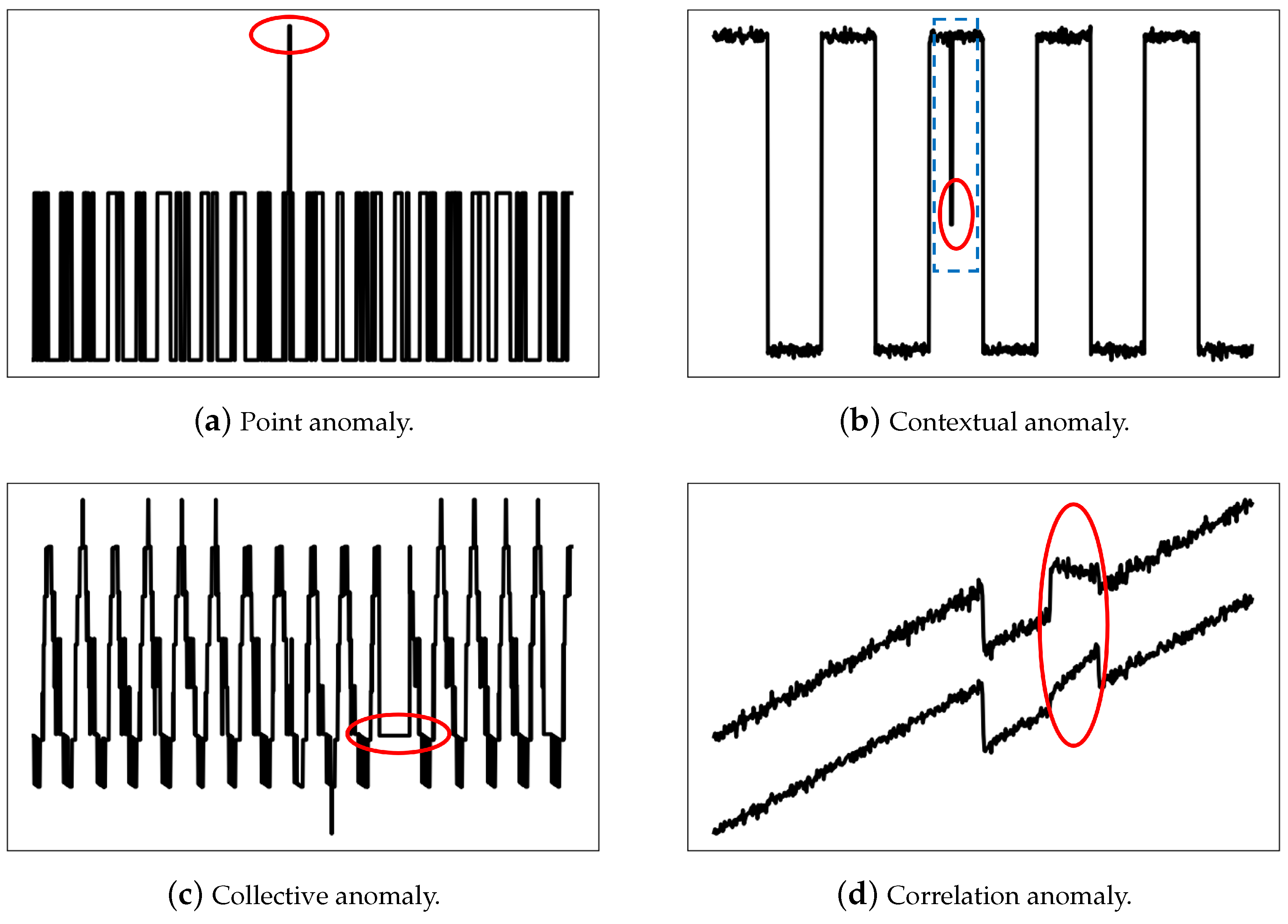
3.1. Categories of Anomalies in Telemetry Data
3.2. Contrastive Learning
4. Proposed Method
4.1. Problem Definition
4.2. Overview of CLPNM-AD Framework
4.3. Data Augmentation
| Algorithm 1: Stochastic augmentation function |
 |
4.4. Representation Learning
4.4.1. One-Dimensional Convolution Encoder
4.4.2. Self-Labeling by Clustering Consistency
4.4.3. Negative Mixing Contrastive Objective
4.5. Score Functions for Detecting Anomaly
5. Experiments
5.1. Datasets
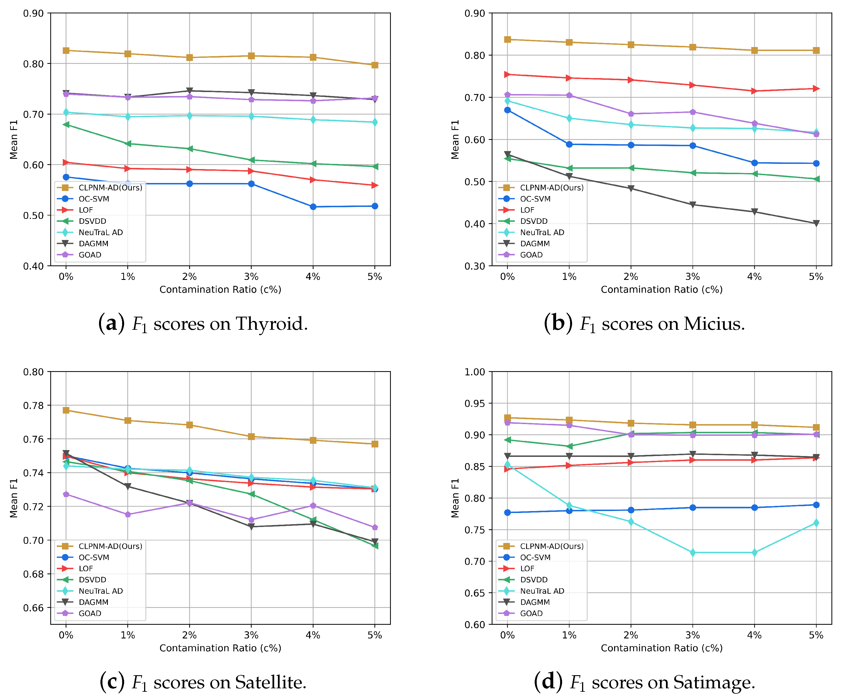
- . The dataset is a thyroid disease classification dataset from the outlier detection datasets (OODS) repository (http://odds.cs.stonybrook.edu/thyroid-disease-dataset/, (accessed on 29 March 2023)), which contains six continuous attributes. The original dataset contains three classes. As hyperfunction is a minority, researchers in the field of anomaly detection treat hyperfunction as anomaly class.
- . The dataset is from the telemetry data of China’s Quantum Science Experiment Satellite, also known as Micius (https://doi.org/10.57760/sciencedb.o00009.00042, (accessed on 29 March 2023)), which contains 19 attributes, and the time span is from January 2017 to February 2019. Micius has four operation patterns. As pattern 4 is rare, we treat pattern 4 as anomaly class and the rest as normal class.
- . The Satellite dataset is integrated by Landsat Satellite from the OODS repository (http://odds.cs.stonybrook.edu/satellite-dataset/, (accessed on 29 March 2023)). Data from three minority categories, 2, 4 and 5, are combined to form the anomaly class, while the remaining classes are combined to form the normal class.
- . The Satimage-2 dataset is from the OODS repository (http://odds.cs.stonybrook.edu/satimage-2-dataset/, (accessed on 29 March 2023)) and is also integrated from Landsat Satellite. Combining the training and test data in the Landsat Satellite dataset, there are 71 outliers in class 2 and all other classes are merged into a normal class.
5.2. Baseline Methods
- OC-SVM [23]. One-Class Support Vector Machine (OC-SVM) is a classical kernel-based anomaly detection method that uses normal data to learn a decision boundary in order to distinguish normal from anomalous data.
- LOF [25]. Local Outlier Factor (LOF) uses the degree of isolation of a sample relative to its surrounding neighbors as the anomaly score to achieve the distinction between normal and abnormal data samples.
- DAGMM [11]. Deep Autoencoding Gaussian Mixture Model (DAGMM) consists of a compression network and an estimation network. The autoencoder acts as a compression network to map the samples into the feature space. The obtained feature vectors and the reconstruction error of the compression network are fed to the estimation network to obtain the energy score/anomaly score.
- Deep SVDD [26]. Deep Support Vector Data Description (Deep SVDD) is the deep variant of SVDD, which aims to leverage the feature extraction capabilities of deep learning to learn a hypersphere only using normal data.
- GOAD [17]. GOAD is a classification-based method for detecting anomalies for general data, which obtains anomaly scores by training a classifier on a set of random auxiliary tasks.
- NeuTraL AD [18]. Neural Transformation Learning for Deep Anomaly Detection (NeuTraL AD) uses a set of learnable transform to replace the fixed random affine transform in the previous literature and provides an end-to-end anomaly detection method with loss function in a form similar to the contrastive loss function.
5.3. Evaluation Metrics
5.4. Model Configuration
5.5. Effectiveness Evaluation
5.6. Robustness Evaluation
5.7. Ablation Experiment
5.8. Sensitivity Studies
6. Conclusions
Author Contributions
Funding
Institutional Review Board Statement
Informed Consent Statement
Data Availability Statement
Acknowledgments
Conflicts of Interest
References
- Hassanien, A.E.; Darwish, A.; Abdelghafar, S. Machine learning in telemetry data mining of space mission: Basics, challenging and future directions. Artif. Intell. Rev. 2020, 53, 3201–3230. [Google Scholar] [CrossRef]
- Baireddy, S.; Desai, S.R.; Mathieson, J.L.; Foster, R.H.; Chan, M.W.; Comer, M.L.; Delp, E.J. Spacecraft time-series anomaly detection using transfer learning. In Proceedings of the IEEE/CVF Conference on Computer Vision and Pattern Recognition, Nashville, TN, USA, 19–25 June 2021; pp. 1951–1960. [Google Scholar]
- Ji, X.Y.; Li, Y.Z.; Liu, G.Q.; Wang, J.; Xiang, S.H.; Yang, X.N.; Bi, Y.Q. A brief review of ground and flight failures of Chinese spacecraft. Prog. Aerosp. Sci. 2019, 107, 19–29. [Google Scholar] [CrossRef]
- Ibrahim, S.K.; Ahmed, A.; Zeidan, M.A.E.; Ziedan, I.E. Machine learning methods for spacecraft telemetry mining. IEEE Trans. Aerosp. Electron. Syst. 2018, 55, 1816–1827. [Google Scholar] [CrossRef]
- Aggarwal, C.C. An introduction to outlier analysis. In Outlier Analysis; Springer: Cham, Switzerland, 2017; pp. 1–34. [Google Scholar]
- Pang, G.; Shen, C.; Cao, L.; Hengel, A.V.D. Deep learning for anomaly detection: A review. ACM Comput. Surv. (CSUR) 2021, 54, 1–38. [Google Scholar] [CrossRef]
- Zhang, X.; Mu, J.; Zhang, X.; Liu, H.; Zong, L.; Li, Y. Deep anomaly detection with self-supervised learning and adversarial training. Pattern Recognit. 2022, 121, 108234. [Google Scholar] [CrossRef]
- Yairi, T.; Takeishi, N.; Oda, T.; Nakajima, Y.; Nishimura, N.; Takata, N. A data-driven health monitoring method for satellite housekeeping data based on probabilistic clustering and dimensionality reduction. IEEE Trans. Aerosp. Electron. Syst. 2017, 53, 1384–1401. [Google Scholar] [CrossRef]
- Takeishi, N.; Yairi, T. Anomaly detection from multivariate time-series with sparse representation. In Proceedings of the 2014 IEEE International Conference on Systems, Man, and Cybernetics (SMC), San Diego, CA, USA, 5–8 October 2014; pp. 2651–2656. [Google Scholar]
- Chalapathy, R.; Menon, A.K.; Chawla, S. Anomaly detection using one-class neural networks. arXiv 2018, arXiv:1802.06360. [Google Scholar]
- Zong, B.; Song, Q.; Min, M.R.; Cheng, W.; Lumezanu, C.; Cho, D.; Chen, H. Deep autoencoding gaussian mixture model for unsupervised anomaly detection. In Proceedings of the International Conference on Learning Representations, Vancouver, BC, Canada, 30 April–3 May 2018. [Google Scholar]
- Lv, P.; Yu, Y.; Fan, Y.; Tang, X.; Tong, X. Layer-constrained variational autoencoding kernel density estimation model for anomaly detection. Knowl.-Based Syst. 2020, 196, 105753. [Google Scholar] [CrossRef]
- Jin, W.; Sun, B.; Li, Z.; Zhang, S.; Chen, Z. Detecting anomalies of satellite power subsystem via stage-training denoising autoencoders. Sensors 2019, 19, 3216. [Google Scholar] [CrossRef]
- Schlegl, T.; Seeböck, P.; Waldstein, S.M.; Schmidt-Erfurth, U.; Langs, G. Unsupervised anomaly detection with generative adversarial networks to guide marker discovery. In Proceedings of the Information Processing in Medical Imaging: 25th International Conference, IPMI 2017, Boone, NC, USA, 25–30 June 2017; pp. 146–157. [Google Scholar]
- Yu, J.; Song, Y.; Tang, D.; Han, D.; Dai, J. Telemetry data-based spacecraft anomaly detection with spatial–temporal generative adversarial networks. IEEE Trans. Instrum. Meas. 2021, 70, 1–9. [Google Scholar] [CrossRef]
- Geiger, A.; Liu, D.; Alnegheimish, S.; Cuesta-Infante, A.; Veeramachaneni, K. Tadgan: Time series anomaly detection using generative adversarial networks. In Proceedings of the 2020 IEEE International Conference on Big Data (Big Data), Atlanta, GA, USA, 10–13 December 2020; pp. 33–43. [Google Scholar]
- Bergman, L.; Hoshen, Y. Classification-based anomaly detection for general data. arXiv 2020, arXiv:2005.02359. [Google Scholar]
- Qiu, C.; Pfrommer, T.; Kloft, M.; Mandt, S.; Rudolph, M. Neural Transformation Learning for Deep Anomaly Detection Beyond Images. In Proceedings of the 38th International Conference on Machine Learning, Online, 18–24 July 2021; Volume 139, pp. 8703–8714. [Google Scholar]
- Chen, T.; Kornblith, S.; Norouzi, M.; Hinton, G. A simple framework for contrastive learning of visual representations. In Proceedings of the International Conference on Machine Learning, Online, 13–18 July 2020; pp. 1597–1607. [Google Scholar]
- Jaiswal, A.; Babu, A.R.; Zadeh, M.Z.; Banerjee, D.; Makedon, F. A survey on contrastive self-supervised learning. Technologies 2020, 9, 2. [Google Scholar] [CrossRef]
- Wang, F.; Liu, H. Understanding the behaviour of contrastive loss. In Proceedings of the IEEE/CVF Conference on Computer Vision and Pattern Recognition, Seattle, WA, USA, 14–19 June 2021; pp. 2495–2504. [Google Scholar]
- Ahmed, T. Online anomaly detection using KDE. In Proceedings of the GLOBECOM 2009-2009 IEEE Global Telecommunications Conference, Honolulu, HI, USA, 30 November–4 December 2009; pp. 1–8. [Google Scholar]
- Li, K.L.; Huang, H.K.; Tian, S.F.; Xu, W. Improving one-class SVM for anomaly detection. In Proceedings of the 2003 International Conference on Machine Learning and Cybernetics (IEEE Cat. No. 03EX693), Xi’an, China, 5 November 2003; Volume 5, pp. 3077–3081. [Google Scholar]
- Li, L.; Hansman, R.J.; Palacios, R.; Welsch, R. Anomaly detection via a Gaussian Mixture Model for flight operation and safety monitoring. Transp. Res. Part C Emerg. Technol. 2016, 64, 45–57. [Google Scholar] [CrossRef]
- Breunig, M.M.; Kriegel, H.P.; Ng, R.T.; Sander, J. LOF: Identifying Density-Based Local Outliers. SIGMOD Rec. 2000, 29, 93–104. [Google Scholar] [CrossRef]
- Ruff, L.; Vandermeulen, R.; Goernitz, N.; Deecke, L.; Siddiqui, S.A.; Binder, A.; Müller, E.; Kloft, M. Deep one-class classification. In Proceedings of the International Conference on Machine Learning, Stockholm, Sweden, 10–15 July 2018; pp. 4393–4402. [Google Scholar]
- Sohn, K.; Li, C.L.; Yoon, J.; Jin, M.; Pfister, T. Learning and evaluating representations for deep one-class classification. arXiv 2020, arXiv:2011.02578. [Google Scholar]
- Tack, J.; Mo, S.; Jeong, J.; Shin, J. Csi: Novelty detection via contrastive learning on distributionally shifted instances. Adv. Neural Inf. Process. Syst. 2020, 33, 11839–11852. [Google Scholar]
- van den Oord, A.; Li, Y.; Vinyals, O. Representation learning with contrastive predictive coding. arXiv 2018, arXiv:1807.03748. [Google Scholar]
- Wu, Z.; Xiong, Y.; Yu, S.X.; Lin, D. Unsupervised feature learning via non-parametric instance discrimination. In Proceedings of the IEEE Conference on Computer Vision and Pattern Recognition, Salt Lake City, UT, USA, 18–23 June 2018; pp. 3733–3742. [Google Scholar]
- He, K.; Fan, H.; Wu, Y.; Xie, S.; Girshick, R. Momentum contrast for unsupervised visual representation learning. In Proceedings of the IEEE/CVF Conference on Computer Vision and Pattern Recognition, Seattle, WA, USA, 14–19 June 2020; pp. 9729–9738. [Google Scholar]
- Caron, M.; Misra, I.; Mairal, J.; Goyal, P.; Bojanowski, P.; Joulin, A. Unsupervised learning of visual features by contrasting cluster assignments. Adv. Neural Inf. Process. Syst. 2020, 33, 9912–9924. [Google Scholar]
- Kalantidis, Y.; Sariyildiz, M.B.; Pion, N.; Weinzaepfel, P.; Larlus, D. Hard negative mixing for contrastive learning. Adv. Neural Inf. Process. Syst. 2020, 33, 21798–21809. [Google Scholar]
- Robinson, J.; Chuang, C.Y.; Sra, S.; Jegelka, S. Contrastive learning with hard negative samples. arXiv 2020, arXiv:2010.04592. [Google Scholar]
- Chuang, C.Y.; Robinson, J.; Lin, Y.C.; Torralba, A.; Jegelka, S. Debiased contrastive learning. Adv. Neural Inf. Process. Syst. 2020, 33, 8765–8775. [Google Scholar]
- Huynh, T.; Kornblith, S.; Walter, M.R.; Maire, M.; Khademi, M. Boosting contrastive self-supervised learning with false negative cancellation. In Proceedings of the IEEE/CVF Winter Conference on Applications of Computer Vision, Waikoloa, HI, USA, 3–8 January 2022; pp. 2785–2795. [Google Scholar]
- Thota, M.; Leontidis, G. Contrastive domain adaptation. In Proceedings of the IEEE/CVF Conference on Computer Vision and Pattern Recognition, Nashville, TN, USA, 20–25 June 2021; pp. 2209–2218. [Google Scholar]
- Lin, S.; Liu, C.; Zhou, P.; Hu, Z.Y.; Wang, S.; Zhao, R.; Zheng, Y.; Lin, L.; Xing, E.; Liang, X. Prototypical graph contrastive learning. IEEE Trans. Neural Netw. Learn. Syst. 2022. [Google Scholar] [CrossRef] [PubMed]
- Bahri, D.; Jiang, H.; Tay, Y.; Metzler, D. Scarf: Self-supervised contrastive learning using random feature corruption. arXiv 2021, arXiv:2106.15147. [Google Scholar]
- Asano, Y.M.; Rupprecht, C.; Vedaldi, A. Self-labelling via simultaneous clustering and representation learning. arXiv 2019, arXiv:1911.05371. [Google Scholar]
- Cuturi, M. Sinkhorn distances: Lightspeed computation of optimal transport. Adv. Neural Inf. Process. Syst. 2013, 26, 1–9. [Google Scholar]
- Gidaris, S.; Singh, P.; Komodakis, N. Unsupervised representation learning by predicting image rotations. arXiv 2018, arXiv:1803.07728. [Google Scholar]
- Lee, K.; Lee, K.; Lee, H.; Shin, J. A simple unified framework for detecting out-of-distribution samples and adversarial attacks. In Proceedings of the Advances in Neural Information Processing Systems 31 (NeurIPS 2018), Montreal, QC, Canada, 3–8 December 2018. [Google Scholar]
- Kamoi, R.; Kobayashi, K. Why is the mahalanobis distance effective for anomaly detection? arXiv 2020, arXiv:2003.00402. [Google Scholar]


| Dataset | Dimensions | Instances | Anomaly Ratio () |
|---|---|---|---|
| Thyroid | 6 | 3772 | 0.025 |
| Micius | 19 | 11250 | 0.200 |
| Satellite | 36 | 6435 | 0.316 |
| Satimage | 36 | 5803 | 0.012 |
| Operation | Units | Activation Function | ||||
|---|---|---|---|---|---|---|
| Thyroid | Micius | Satellite | Satimage | |||
| Encoder | Linear | (6, 128) | (19, 128) | (36, 128) | (36, 128) | LeakyReLU(0.2) |
| Reshape | (*, 16, 8) | (*, 16, 8) | (*, 16, 8) | (*, 16, 8) | ||
| Conv1d | (16, 32, 1) | (16, 32, 1) | (16, 32, 1) | (16, 32, 1) | ||
| BatchNorm1d | (32) | (32) | (32) | (32) | LeakyReLU(0.2) | |
| Conv1d | (32, 6, 1) | (32, 32, 1) | (32, 36, 1) | (32, 256, 1) | ||
| BatchNorm1d | (6) | (32) | (36) | (256) | LeakyReLU(0.2) | |
| Conv1d | (6, 6, 1) | (32, 32, 1) | (36, 36, 1) | (256, 256, 1) | ||
| BatchNorm1d | (6) | (32) | (36) | (256) | ||
| Flatten | LeakyReLU(0.2) | |||||
| Linear | (48, 6) | (256, 32) | (288, 36) | (2048, 256) | LeakyReLU(0.2) | |
| Projection Head | Linear | (6, 6) | (32, 32) | (36, 36) | (256, 256) | |
| Prototypes (C) | Linear | (6, 4) | (32, 8) | (36, 4) | (256, 12) | |
| Method | Dataset | |||
|---|---|---|---|---|
| Thyroid | Micius | Satellite | Satimage | |
| OC-SVM [23] | ||||
| LOF [25] | ||||
| DAGMM [11] | ||||
| DSVDD [26] | ||||
| GOAD [17] | ||||
| NeuTraL AD [18] | ||||
| CLPNM-AD (Ours) | ||||
| Dataset | Method | |||||
|---|---|---|---|---|---|---|
| OC-SVM | LOF | DAGMM | DSVDD | GOAD | NeuTraL AD | |
| Thyroid | ||||||
| Micius | ||||||
| Satellite | ||||||
| Satimage | ||||||
| Datasets | ||||||
|---|---|---|---|---|---|---|
| Negatives Mixing | Thyroid | Micius | Satellite | Satimage | ||
| ✔ | 63.3 ± 5.0 | 83.2 ± 1.1 | 74.8 ± 0.3 | 91.4 ± 1.0 | ||
| ✔ | 75.4 ± 3.5 | 83.1 ± 1.3 | 75.5 ± 8.3 | 92.6 ± 1.9 | ||
| ✔ | ✔ | 80.3 ± 1.9 | 83.2 ± 1.2 | 75.7 ± 0.6 | 91.5 ± 2.5 | |
| ✔ | ✔ | ✔ | 82.6 ± 3.0 | 83.7 ± 1.1 | 77.7 ± 0.5 | 92.7 ± 1.3 |
Disclaimer/Publisher’s Note: The statements, opinions and data contained in all publications are solely those of the individual author(s) and contributor(s) and not of MDPI and/or the editor(s). MDPI and/or the editor(s) disclaim responsibility for any injury to people or property resulting from any ideas, methods, instructions or products referred to in the content. |
© 2023 by the authors. Licensee MDPI, Basel, Switzerland. This article is an open access article distributed under the terms and conditions of the Creative Commons Attribution (CC BY) license (https://creativecommons.org/licenses/by/4.0/).
Share and Cite
Guo, G.; Hu, T.; Zhou, T.; Li, H.; Liu, Y. Contrastive Learning with Prototype-Based Negative Mixing for Satellite Telemetry Anomaly Detection. Sensors 2023, 23, 4723. https://doi.org/10.3390/s23104723
Guo G, Hu T, Zhou T, Li H, Liu Y. Contrastive Learning with Prototype-Based Negative Mixing for Satellite Telemetry Anomaly Detection. Sensors. 2023; 23(10):4723. https://doi.org/10.3390/s23104723
Chicago/Turabian StyleGuo, Guohang, Tai Hu, Taichun Zhou, Hu Li, and Yurong Liu. 2023. "Contrastive Learning with Prototype-Based Negative Mixing for Satellite Telemetry Anomaly Detection" Sensors 23, no. 10: 4723. https://doi.org/10.3390/s23104723
APA StyleGuo, G., Hu, T., Zhou, T., Li, H., & Liu, Y. (2023). Contrastive Learning with Prototype-Based Negative Mixing for Satellite Telemetry Anomaly Detection. Sensors, 23(10), 4723. https://doi.org/10.3390/s23104723