Abstract
Accurate prediction of aviation safety levels is significant for the efficient early warning and prevention of incidents. However, the causal mechanism and temporal character of aviation accidents are complex and not fully understood, which increases the operation cost of accurate aviation safety prediction. This paper adopts an innovative statistical method involving a least absolute shrinkage and selection operator (LASSO) and long short-term memory (LSTM). We compiled and calculated 138 monthly aviation insecure events collected from the Aviation Safety Reporting System (ASRS) and took minor accidents as the predictor. Firstly, this paper introduced the group variables and the weight matrix into LASSO to realize the adaptive variable selection. Furthermore, it took the selected variable into multistep stacked LSTM (MSSLSTM) to predict the monthly accidents in 2020. Finally, the proposed method was compared with multiple existing variable selection and prediction methods. The results demonstrate that the RMSE (root mean square error) of the MSSLSTM is reduced by 41.98%, compared with the original model; on the other hand, the key variable selected by the adaptive spare group lasso (ADSGL) can reduce the elapsed time by 42.67% (13 s). This shows that aviation safety prediction based on ADSGL and MSSLSTM can improve the prediction efficiency of the model while keeping excellent generalization ability and robustness.
1. Introduction
The aviation industry is of great economic value, and to adapt to the current demand for intelligent and refined safety management, the aviation safety mitigation strategy has been shifting from a reactive to a proactive and predictive method. Therefore, it is greatly significant to clarify the causal mechanisms of aviation accidents and make corresponding early warning measures to promote the development of aviation safety.
Accurate aviation safety prediction is the basis of effective accident early warning, which has become a hot topic of research today. Recently, the aviation safety prediction method used specific machine learning methods to train the features of historical causes and accident samples, construct a mathematical analytical model, and measure the change trend of the safety level. For example, Liang et al. [1] used the BP (backpropagation) neural network model to predict the monthly incidents per 10,000 flight hours of an airline. Puranik et al. [2] built an online predictive model based on a Random Forest regression algorithm to predict landing performance metrics. Rosa et al. [3] constructed an aviation safety risk assessment model based on the Bayesian inference mechanism. Lukacova et al. [4] proposed a model for accident severity prediction based on classification and regression trees. Zhang et al. [5] proposed a combined method involving SVM (support vector machine) and deep neural networks to qualify the risk. Qiao et al. [6] constructed the RBF (radial basis function) neural network model to predict the hard landing. Machine learning not only has strong self-learning ability and robustness but also can better fit the nonlinear relationships among complex variables. However, the input variables of traditional machine learning models are generally regarded stand-alone, that is, the temporal features are not fully taken into consideration, which adds interference to the prediction results. To fully extract the temporal features, Xiong et al. [7] used LSTM neural network model to train and predict the sign data of American bird strike accidents. However, single-layer structures are adopted in that paper, and it’s difficult to accurately integrate the nonlinear relationships. Zhou et al. [8] used the ACARS (aircraft communications addressing and reporting system) accident report record as the research object, using the LSTM model to effectively capture the long-term dependency of samples and enhance the accuracy and robustness of safety measurement. Zhang [9] applied sequential deep learning techniques based on LSTM to perform a prognosis of adverse events. While the aviation accident data is typically a small sample, it’s difficult to efficiently learn sample characteristics by peer-to-peer prediction.
In addition to the selection of prediction methods, the selection of input variables affects the predicted effect. The classic accident inducement identification model is represented by the SHEL [10] model, REASON [11], HFACS [12] (human factors analysis classification system), OHFAM [13] (occurrence human factors analysis model) and 24 model [14]. The expansion of the inducement index is theoretically conducive to obtaining a more accurate causality description but brings the curse of dimensionality accordingly: the higher the dimensions of the input set are, the efficiency of safety prediction will be greatly reduced. Existing studies have led to some explorations in variable selection: Paulet al. [15], in the form of a questionnaire interview, intuitively modeled the greatest threat from the perspective of pilots. Cui et al. [16] used DEA (data envelope analysis) and a Malmquist index to calculate the civil aviation safety efficiency of Chinese airlines from 2008 to 2012, it proved that the quality of personnel training is the most important factor affecting aviation safety. In view of the high-dimensional samples with multiple collinearities, some scholars have tried to introduce the LASSO penalty term in the classic regression model. LASSO can greatly compress the value of independent variables to dilute the high-dimensional aviation data, which verifies the feasibility in the field of fuel consumption [17]. However, there is still a blank in the inducement of aviation accident variable selection. Meanwhile, the classic LASSO punishes the coefficient of key variables consistently, which weakens the feature identification of those key variables.
In view of the status that existing methods have an insufficient description of the importance of aviation accidents and low prediction efficiency, this paper proposes a new method of aviation safety prediction based on variable selection and LSTM. The contributions of the proposed method can be described as follows: (a) the dimensions of the security sample data are sufficiently reduced [18] by ADSGL, which reduces the cost of a running predictor and the elapsed time. (b) the multistep stacked LSTM model is constructed to explore the deep temporal features and complex nonlinear relationship of aviation safety samples and achieve smaller RMSE compared with the original model.
The rest of this paper is organized as follows: Section 2 describes the required individual algorithms and the process for building the proposed methods. Section 3 demonstrates a case study, followed by the training process for the constructed model. Section 4 provides a comparative analysis to verify the feasibility and effectiveness of the proposed method, and Section 5 presents the conclusions.
2. Proposed Aviation Safety Prediction Method
2.1. The Whole Process of the Proposed Method
The process of the ADSGL-MSSLSTM method is depicted in Figure 1. The detailed descriptions are given as follows:
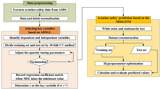
Figure 1.
Flow chat of the ADSGL-MSSLSTM method.
(1) Data preprocess. Firstly, the aviation safety data are collected by the type of incidents from ASRS [19] reporting records, thus the text data is converted into structured data. Next, the aviation safety data is normalized into the range of [0, 1] to eliminate the interference of dimensional differences in data analysis.
(2) Key variables selection based on ADSGL. In view of the fact that there are too many manipulated variables to efficiently build predictive models, ADSGL is used to select key variables. The selected key variables are regarded to have the most interpretable information for incidents, which effectively reduces the operating cost and improves the calculation efficiency.
(3) Aviation safety prediction based on the MSSLSTM. In view of the fact that the predictors ignore the temporal dependence, which reduces the interpretability and accuracy, a multistep prediction model of aviation safety based on a multi-layer LSTM is constructed. Firstly, the white noise and stationarity of the data are tested. Secondly, the sample set is reconstructed to match the supervised learning mode. Thirdly, to enhance the ability of nonlinear fitting and temporal characteristic extraction, the hidden layer depth and learning step are adjusted, as well the learning error minimization is the criterion of optimal parameter establishment.
2.2. Selection of Aviation Safety Inducement Variables Based on ADSGL
2.2.1. LASSO Penalty Operator
For the classic linear regression model [20] for aviation safety level, we defined it by
where is the n-dimensional response variable vector, and is the n*l-dimensional explanatory variable matrix. is the regression coefficient matrix, the distribution of error is followed as .
The sum of the error is taken as the loss function, the penalized likelihood estimation [21] (objective function) is defined as
where is the 2-Norm, penalized expressions for a single input variable are usually expressed as , 0 < q ≤ 2. The penalty term is called the LASSO penalty when q = 1. λ is the adjustable coefficient, which can be adjusted to obtain the optimal solution and scale the penalty term appropriately.
The advantages brought by the LASSO penalty into the inducements variable selection of aviation incidents can be illustrated as follows [22].
(1) Increase the sparsity of the regression coefficient matrix. Sparsity refers to the existence of several sample points with a value of 0, which conforms to the actual selection of incident inducement variables; when a candidate variable is an irrelevant interference variable, the corresponding regression coefficient is 0. The is strictly equal to 0 when λ takes a large value, so as to realize the sparsity of the coefficient matrix and to achieve the variable selection.
(2) Increase in model stability. The input variable matrix is often followed by multicollinearity, and the obtained result may be non-inferior, which only satisfies the local optima. Daubechies, Defrise and De Mol [23] prove that any penalty for the coefficient matrix satisfying 1 ≤ p ≤ 2 can make the solution of the original model more stable.
However, the classic LASSO algorithm still has obvious defects: when making a univariate selection, LASSO agrees with the shrinkage multiple of the regression coefficient, which will impose more penalty on the coefficient term, resulting in the inconsistency and bias of the dimensionality reduction model.
2.2.2. Construction of the Algorithm for Aviation Safety Variable Selection
To address some limitations of the classic LASSO algorithm, this paper adopts a variable selection method based on the adaptive sparse group LASSO: when optimizing the minimum loss function, the function is univariate, that is, to adapt to the various inducement variables and the vastly different punishment strategy features, only one variable is optimized each time and cycled repeatedly until all variables converge.
l explanatory variables are divided into N non-overlapping groups. The objective function of ADSGL is formulated as
where is the weight matrix explaining the group variables, is the weight matrix explaining the univariate. The weight matrix introduced by ADSGL can effectively reduce the penalty of the biggish coefficient, which keeps the model consistent and unbiased and improves the accuracy of variable selection. The algorithmic steps are summarized as follows:
Step 1 the initial value of the regression coefficient is set as
Step 2 for k = 1, 2, …, N, if k satisfies the (5), then ; Otherwise, turn to the Step 3.
is defined as
Step 3 In the k th group of the regression coefficient, for , if k satisfies the (8), then ; Otherwise, turn to the Step 4.
Step 4 is taken in (9) to solve the optimized regression coefficient values.
Step 5 The threshold of absolute error is set and Step 2~Step 4 is cycled until convergence. The convergence algorithm is expressed as
where f0 is a strictly convex function and can be differentially. The algorithm avoids premature convergence and falling into a local optimum [24], and dynamically adjusts the penalty term according to the size of the regression coefficient, effectively reducing the calculation errors.
2.3. Aviation Safety Prediction Based on LSTM Neural Network
2.3.1. LSTM Architecture
To evaluate the selected key variables in improving the prediction accuracy, the LSTM architecture is used as an aviation safety predictor. The LSTM architecture has a memory unit and forget gate, which can update the cell state in real-time: the previous output (ht−1) and the current input (xt) enter the forget gate and determines how much information is forgotten from the previous state (ct−1). Accordingly, the input gate determines how much the updated state is retained in the current state (ct); the output gate determines how much information the ct export, thus continuously updating the state parameters over time. The network architecture of LSTM is shown in Figure 2.
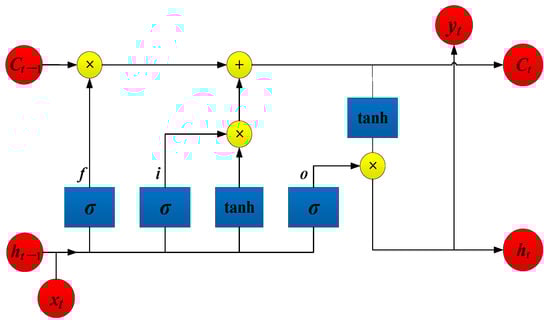
Figure 2.
The network architecture of LSTM.
Where f is the forget gate, i is the input gate, and o is the output gate. is the incentive function, which generally takes the sigmoid function. The tanh is a hyperbolic tangent function. sigmoid and hyperbolic tangent function can be implemented as
The updated formulas [25] for each gate and cell state can be implemented as
where W is the weight of xt, U is the weight of ht−1, b is the biases, is the critical state of the cell.
When processing the RNN model, the iterations of BPTT (backpropagation through time) increase due to the higher amounts of steps, which is most likely to initiate the gradient disappearance so that each parameter cannot be accurately updated. However, the unique gate structure of LSTMs can better alleviate such problems. BPTT can be implemented as
where Jt represents the cumulative training loss from the start to the current moment. In RNN: and the value is [0, 1/4]. While in LSTM: and the value is [0, 1]. When the training time is too long, the cumulative effect makes the training gradient of RNN tend to 0, greatly reducing the learning rate. LSTM can control at about 1, to prevent the gradient disappearance or explosion, and ensure the accurate update of parameters.
2.3.2. Prediction Process
- (1)
- Stationarity and white noise test
The research object of the LSTM predictor is a temporal aviation safety sample, so the stationarity and white noise of the sample should be tested first, and the tested sample can be analyzed and predicted by the predictor.
A stationary sequence refers to a temporal sample with no obvious volatility, trend, or cyclicity. A white noise sequence is randomly generated and mutually uncorrelated, and it is characterized by 3 features:
1) E(xt = 0); 2) D(xt) = σ2; 3) Cov(xt, xt + k) = 0 (k 0). A schematic drawing of white noise sequence is shown in Figure 3.
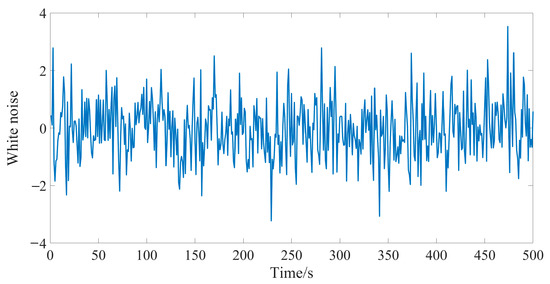
Figure 3.
Sequence diagram for white noise.
- (2)
- Refactoring the data
Input and output feature vectors (xt, yt) are refactored and fit into the sequence-to-sequence learning in the LSTM network: xt and yt−1 (t = 2,…, n) are merged as.
The training set is also divided according to each step size.
The test set is refactored as.
where n is the sum of the time steps, p is the length of the input sample, and q is the length of the output sample.
- (3)
- Constructing a multistep stacked predictor of aviation safety
Peer to peer prediction adopted by the original LSTM cannot accurately describe the changes of the aviation safety level. Additionally, a single layer network lacks the ability to capture the temporal dependence of dataset. To address the above problems, the training layers and step size of the classic LSTM model are adjusted. The MSSLSTM model is constructed in turn, as shown in Figure 4.
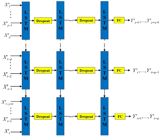
Figure 4.
Aviation safety prediction model based on MSSLSTM.
In the same training batch, the number of hidden layers neuron is set as k, and the number of hidden layers is set as l. The output of the previous hidden layer is used as the input of the current layer, the dropout layer is set between adjacent hidden layers to reduce the model complexity, and the last hidden layer and output termination are fully connected [26]. Finally, the n-dimensional output vector is activated by the softmax function. The fully connected layer can be implemented as.
The multistep stacked LSTM predictor not only increases the input sizes, which helps calculate the digital features of multiple historical samples in the input gate, improving the usage of existing samples but also increases the length of the output sample, which helps to describe the change trend of the aviation safety level more intuitively. Compared with the original LSTM model, the multistep stacked LSTM predictor strengthens the cell’s learning performance on the temporal features, explains the trendy changes in safety level more visually, and helps conduct better forward-looking and real-time prediction. Additionally, the stacked architecture not only greatly strengthens the deep learning ability, but improves the robustness and adaptability of the predictor.
- (4)
- Optimizing hyperparameters
The learning rate is optimized by the Adam algorithm with weight decay, the number of hidden layers and nodes are ergodic by step search, the MAE (mean absolute error) of the training results are compared under different parameter combinations, and it is recorded when the MAE takes the minimum value.
MAE can be implemented as
where is the test value, is the predicted value.
The Adam optimization process is as follows.
Firstly, the first-order and second-order moment estimation of the gradient is calculated:
where and are decay rates for the first-order and second-order moment estimates.
Secondly, the deviation term of the correction moment estimate is calculated:
Finally, the learning rate update value is calculated based on the correction:
where is the initial learning rate. Adam controls the updated learning rate in the measurable range, and accelerates the collection speed and ensures the robustness of the model.
- (5)
- Model accuracy evaluation
To intuitively evaluate the accuracy of the prediction model, single layer-multistep LSTM (LSTM’), the original LSTM, MSSRNN, TCN (temporal convolutional network), DT (decision tree), SVR (support vector regression), and ARMA (autoregressive moving average) predictors are used as control models to compute in the same experimental environment. RMSE is used as the accuracy evaluation indicator. RMSE can be implemented as
3. Examples of Aviation Safety Predictions Based on Variable Selection and LSTM
3.1. Data Preprocessing
The study sample was taken from ASRS. The complete report record [27] includes Time, Environment, Aircraft, Component (faulty parts, accident recorded with mechanical failure), Person, Events, Assessments, and Synopsis. The text data example is shown in Table 1.

Table 1.
An example of the safety report taken from ASRS.
According to the description of Assessments and Synopsis in the reports, the variables of the accident dataset can be classified into 12 input variables: aircraft (A), company policy (CP), procedure (P), weather (W), communication breakdown (CB), confusion (C), distraction (D), human-machine interface (HMC), situational awareness (SA), time pressure (TP), training/qualification (TQ), workload (WL), and 1 output variable: minor accident (MA). Based on this, the monthly statistics of accidents from June 2010 to Nov 2020 were collected.
To eliminate the interference from dimensional differences [28], the dataset was normalized by min-max normalization. The normalized index values were scaled linearly between 0 and 1. The min-max normalization can be implemented as.
where xmax and xmin represent the maximum and minimum values of the sample, x is the original value, x* is the normalized value. Normalized results are shown in Table 2.
Table 2.
Normalized results.
The differences in value distributions were eliminated in the normalized sample, and the numerical features are retained by equal scale.
3.2. Selection of Key Variables Based on the ADSGL
3.2.1. Setting of the Key Parameters of the Variable Selection Algorithm
The aircraft incident in Table 3 was selected as the dependent variable and denoted by ; The remaining 12 types of insecure events were selected as the independent variable and denoted by . To improve the usage of the sample while avoiding overfitting [29], 10-fold cross-validation was used to divide the dataset. Given the actual sample size, the epoch was set at 100, and the number of groups was set at 2. To ensure the credibility of the experimental results, the variable selection was performed in the different relaxed variables (α). Parameters settings are shown in Table 3.
Table 3.
Parameter settings of the ADSGL algorithm.
3.2.2. Analysis of Experimental Results
Minimum MSE (mean square error) is selected as the final selection results. MSE can be implemented as.
The experimental results are shown in Figure 5.
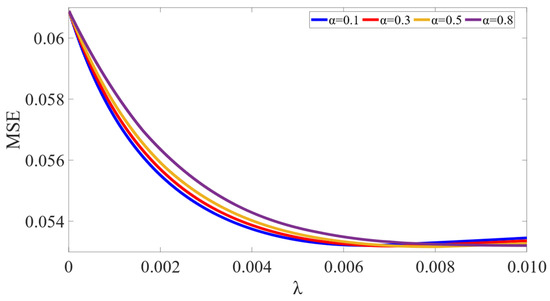
Figure 5.
Changes of the validation MSE under the different relaxation variables.
Figure 5 shows the changes in the validation MSE with λ increasing. As are set to 0.1, 0.3, 0.5, 0.8, the minimum MSE values in these 4 groups of experiments all are around 0.05, and the convergence speeds up as alpha increases, which reflects the good robustness of ADSGL in terms of error convergence, and a strong positive correlation is implicated between alpha and convergence speed. Lasso fitting coefficient tracer diagram as α takes 0.1 is shown in Figure 6.
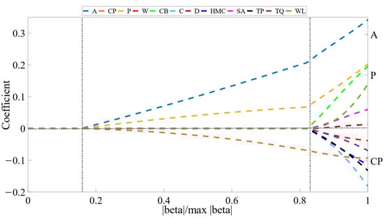
Figure 6.
Lasso fitting coefficient tracer diagram as α takes 0.1.
From Figure 6, it can be seen that: One group of variables’ coefficients (W, CB, C, D, HMC, SA, TP, TQ, WL) converged at a higher rate compared with the other group (A, CP, P), which indicates that the variables in the latter group are still highly interpretable to the output variables at optimal penalty weight. The absolute values of coefficients, which in the first group converged, are depicted in Figure 7.
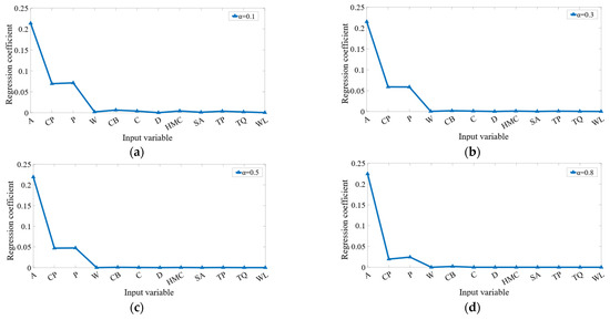
Figure 7.
The absolute values of compressed regression coefficients as α set to (a) 0.1, (b) 0.3, (c) 0.5, (d) 0.8.
From Figure 7, it can be found that the values of compressed regression coefficients are relatively consistent when the is adjusted, which demonstrates that the ADSGL method is robust in the contraction of regression coefficients. Furthermore, the common intersection set of the results of the four experimental are {A, CP, P}, the regression coefficients of which are non-zero in the largest penalty, having a greater impact on the MA. Therefore, those three variables are selected as the input variables of the aviation safety predictor.
3.3. Multistep Aviation Safety Prediction Based on the MSSLSTM Model
3.3.1. Dataset Refactoring
After passing the white noise and stationarity test, the dataset was refracted and fit into the supervised learning form of the LSTM network: xt was merged with yt−1 (t = 2,…, n) into the feature set, which can be implemented as , and the output set was .
The training step was generally fixed in the learning process and set based on actual demand, given the significant temporal dependence of aviation accidents, the lengths of the input and output samples were set to 4: the historical data of the last 4 months were used to predict the safety level in the next 4 months. The training and test sets were divided accordingly:
3.3.2. Stability Test and White Noise
To visually present the trend features of the sample over time, each variable was analyzed. The sequence diagram for the insecure events is presented in Figure 8.
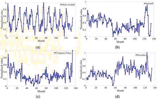
Figure 8.
Sequence diagram for (a) MA, (b), A (c) CP, (d) P.
Figure 8a shows that the sample variance of the minor accident is stable overall. The sequence has little volatility, and no obvious trend and cyclicity, so it can be regarded as a stationary sequence. Additionally, the expectation for the sample is much larger than 0, which does not satisfy the autocorrelation property of a white-noise sequence. Thus, the sample passed the white noise test.
In turn, the other variables were observed in turn according to the sequence diagram, the results show that all input and output variables were stationary and non-white-noise sequences.
3.3.3. Hyperparameter Optimization
To observe the predicted effect of the model at different batches, the number of nodes and number of layers were successively adjusted. To alleviate the overfitting, neurons were randomly discarded at 65% for each training session (dropout_rate = 0.65).
Furthermore, we adjusted the number of layers, constructed the MSSLSTM aviation safety predictor, and traversed the training error (MAE). Figure 9 shows that the MAE decreases as the layer number increases to 4 and the minimum MAE is about 0.1962, which demonstrates that the stacked structure enhances the deep learning ability. While MAE increases as the layer number is over 4, the possible cause is overfitting due to model complexity. Thus, the number of hidden layers in this case was set as 4.
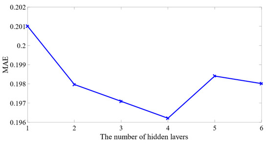
Figure 9.
Changes of training accuracy under different number of layers.
Figure 10a shows the changes in training errors under the number of nodes combination of the first two layers. It shows that the global minimum MAE is about 0.1917, as the number of nodes were set as 9 and 7.
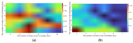
Figure 10.
Changes of training accuracy under different number of nodes in the (a) 1st and 2nd hidden layer, (b) 3rd and 4th hidden layer.
Based on the optimization of the nodes’ number in the first two layers, we adjusted the nodes’ number in the last two layers, training errors are accordingly shown in Figure 10b, the global minimum MAE is about 0.1751, as the number of nodes were set as 5, 5.
From the parameters described above, the optimal setting for the number of nodes was set as 9, 7, 5, 5.
4. Model Comparison
4.1. Effect of Predictors on the Experimental Results
The model proposed in this paper based on the MSSLSTM will be compared with prediction models such as , LSTM, MSSRNN, TCN, DT, SVR, and ARMA. Those compared models were all used to predict the value of aviation safety level in the same experimental environment. The comparison experiment results of each model are shown in Figure 11.
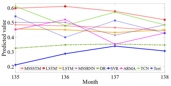
Figure 11.
Comparison of the predictive model results.
From Figure 11, it can be seen that: (1) the MSSLSTM predictor outperforms the original LSTM in the fitting effect. (2) Recurrent neural networks (RNNs) are better than the ARMA model, as it demonstrates a better ability to recognise and understand trends by the memory units. (3) For DR and SVR, the prediction errors have a much wider range of deviations, compared with RNNs, which indirectly proved that RNNs are relatively robust. (4) TCN performs well to fit increasing and decreasing trends of predicted value but has a large relative error.
The RMSE distribution of the 10 experiments is recorded. As shown in Figure 12: (1) The error of MSSLSTM is the least, and RMSE is below 0.058, which is reduced by 41.977% and 28.37% compared with LSTM and TCN. This further proves that the robustness of the MSSLSTM proposed in this paper has been strengthened. (2) The accuracy of the MSSLSTM is slightly higher than that of the MSSRNN, which shows that gate structure helps improve the accuracy of multi-layers predictor.
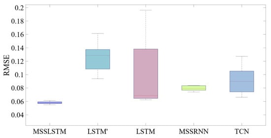
Figure 12.
The RMSE distribution diagram of the ten-time experiments.
4.2. Effect of Variable Selection Methods on the Experimental Results
To more intuitively verify the effectiveness and robustness of ADSGL for improving safety prediction efficiency, LASSO, Group LASSO, ridge regression (RR), and random forest (RF) are introduced into the proposed MSSLSTM predictor, respectively, and the input variables determined by the variable selection methods are tested. The RMSE, elapsed time (t), and the number of selected variables (Variable_number) are used as evaluation indicators.
The comparison experiment results of each model are shown in Table 4.
Table 4.
Comparison of test results with variable selection methods.
It can be seen from the comparison of Table 4 that: (1) The predicted RMSE of ADSGL is 0.058, which is significantly lower than that of the original operator (LASSO, RR), and the convergence error is the minimum. It shows that the accuracy of the proposed ADSGL is greatly improved, compared with the original operator. (2) The accuracy of the ADSGL is better than that of the RF, and the error decreased by more than 35.53%, which verifies the effectiveness of the penalty term in improving the accuracy. (3) Compared with the original LASSO, the elapsed time is shortened by nearly 13 s. It proves that the proposed ADSGL greatly improves elapsed efficiency. (4) The number of variables selected by ADSGL is 3, under the premise of ensuring prediction accuracy, the sample dimensions get fully reduced, by about 63.3%, with better interpretability.
5. Conclusions
This paper presents a new aviation safety prediction method based on ADSGL- MSSLSTM. In this study, ADSGL is used to select key variables based on coefficients’ shrinking at both the group level and univariate level, and penalize the coefficients differently depending on their adaptive weights. In this way, the evaluations are ensured to be unbiased and consistent, which improves selection model accuracy and interpretability. Subsequently, MSSLSTM is trained using a dataset after dimension reduction, and it’s then used to predict the changing trend in minor accidents. The multi-step stacked structure enhances the predictor by generalizing and analyzing complex temporal dependencies and nonlinear relationships, which helps further improve the prediction efficiency and robustness.
The feasibility of ADSGL-MSSLSTM is demonstrated by case studies of data collected in ASRS, from June 2010 to Nov 2020. Various existing methods are determined as control models. Experimental results indicate that the proposed method can efficiently conduct key variable selection and improve the prediction performance of aviation incidents.
As part of the future work, firstly, given the difference in safety among various models of aircraft, we will apply the proposed method to predict the safety level in a specific model, thus extracting more tailored safety information. Additionally, appropriately increasing the appropriate coefficient penalty will be adopted to speed up the error convergence rate while satisfying the accuracy demand.
Author Contributions
Conceptualization, H.Z. (Hang Zeng), J.G. and H.Z. (Hongmei Zhang); methodology, H.Z. (Hang Zeng); investigation, B.R.; data curation, J.W.; writing—original draft preparation, H.Z. (Hang Zeng); writing—review and editing, J.G. and H.Z. (Hongmei Zhang); supervision, B.R. All authors have read and agreed to the published version of the manuscript.
Funding
This work was funded by the Natural Science Foundation of Shangxi Province, China (Grant No. 2019JQ-710).
Institutional Review Board Statement
Not applicable.
Informed Consent Statement
Not applicable.
Data Availability Statement
Not applicable.
Conflicts of Interest
The authors declare no conflict of interest.
References
- Liang, W.J.; Li, X.Y. Flight incidents prediction of air transportation based on the combined model of ARIMA, LS-SVM and BPNN. Saf. Environ. Eng. 2018, 25, 130–136. [Google Scholar]
- Puranik, T.G.; Rodriguez, N.; Mavris, D.N. Towards online prediction of safety-critical landing metrics in aviation using supervised machine learning. Transp. Res. Part C Emerg. Technol. 2020, 120, 102819. [Google Scholar] [CrossRef]
- Rma, V.; Comendador, V.; Sanz, L.P. Prediction of aircraft safety incidents using Bayesian inference and hierarchical structures-ScienceDirect. Saf. Sci. 2018, 104, 216–230. [Google Scholar]
- Lukáčová, A.; Babičand, F.J.; Paralič, J. Building the prediction model from the aviation incident data. In Proceedings of the IEEE International Symposiumon Applied Machine Intelligence & Informatics, Herl’any, Slovakia, 23–25 January 2014; pp. 365–369. [Google Scholar]
- Zhang, X.; Mahadevan, S. Ensemble machine learning models for aviation incident risk prediction. Decis. Support Syst. 2019, 116, 48–63. [Google Scholar] [CrossRef]
- Qiao, X.; Chang, W.; Zhou, S.; Lu, X.F. A prediction model of hard landing based on RBF neural network with K-means clustering algorithm. In Proceedings of the 2016 IEEE International Conference on Industrial Engineering and Engineering Management (IEEM), Bali, Indonesia, 4–7 December 2016; pp. 462–465. [Google Scholar]
- Xiong, M.L.; Wang, H.W.; Xu, Y.; Fu, Q. General aviation safety research based onprediction of bird strike symptom. Syst. Eng. Electron. 2020, 42, 2033–2040. [Google Scholar]
- Zhou, D.; Zhuang, X.; Zuo, H.; Wang, H.; Yan, H. Deep Learning-Based Approach for Civil Aircraft Hazard Identification and Prediction. IEEE Access 2020, 8, 103665–103683. [Google Scholar] [CrossRef]
- Zhang, X.G.; Srinivasan, P.; Mahadevan, S. Sequential deep learning from NTSB reports for aviation safety prognosis. Saf. Sci. 2021, 142, 105390. [Google Scholar] [CrossRef]
- Perboli, G.; Gajetti, M.; Fedorov, S.; Giudice, S.L. Natural language processing for the identification of human factors in aviation accidents causes: An application to the shel methodology. Expert Syst. Appl. 2021, 186, 115694. [Google Scholar] [CrossRef]
- Demirci, S. The requirements for automation systems based on Boeing 737 MAX crashes. Aircr. Eng. Aerosp. Technol. 2022, 94, 140–153. [Google Scholar] [CrossRef]
- Hulme, A.; Stanton, N.A.; Walker, G.H.; Waterson, P.; Salmon, P.M. What do applications of systems thinking accident analysis methods tell us about accident causation? a systematic review of applications between 1990 and 2018. Saf. Sci. 2019, 117, 164–183. [Google Scholar] [CrossRef]
- Rong, M.; Luo, M.; Chen, Y.; Sun, C.; Wang, Y. Human Factor Quantitative Analysis Based on OHFAM and Bayesian Network. In Proceedings of the International Conference on Human-Computer Interaction, HCI International 2014, Heraklion, Crete, Greece, 22–27 June 2014; pp. 533–539. [Google Scholar]
- Fu, G.; Lu, B.; Chen, X.Z. Behavior Based Model for Organizational Safety Management. China Saf. Sci. J. 2005, 15, 21–27. [Google Scholar]
- O’Connor, P.; Cowan, S.; Alton, J. A comparison of leading and lagging indicators of safety in naval aviation. Aviat. Space Environ. Med. 2010, 81, 677–682. [Google Scholar] [CrossRef] [PubMed]
- Cui, Q.; Li, Y. The change trend and influencing factors of civil aviation safety efficiency: The case of Chinese airline companies. Saf. Sci. 2015, 75, 56–63. [Google Scholar] [CrossRef]
- Wang, S.Z.; Ji, B.X.; Zhao, J.S.; Liu, W.; Xu, T. Predicting ship fuel consumption based on LASSO regression. Transp. Res. Part D: Transp. Environ. 2018, 65, 817–824. [Google Scholar] [CrossRef]
- Xie, J.; Hong, T. Variable Selection Methods for Probabilistic Load Forecasting: Empirical Evidence from Seven States of the United States. IEEE Trans. Smart Grid 2018, 9, 6039–6046. [Google Scholar] [CrossRef]
- Zhao, J.C.; Deng, F.; Cai, Y.Y. Long short-term memory-fully connected (LSTM-FC) neural network for pm 2.5 concentration prediction. Chemosphere 2019, 220, 486–492. [Google Scholar] [CrossRef]
- Karmitsa, N.; Taheri, S.; Bagirov, A.; Mäkinen, P. Missing Value Imputation via Clusterwise Linear Regression. IEEE Trans. Knowl. Data Eng. 2022, 34, 1889–1901. [Google Scholar] [CrossRef]
- Xu, Y.J.; Luo, Y.X. VARCLUS-based Principal Component Lasso Dimensionality Reduction Algorithm and Simulation. Stat. Decis. 2021, 4, 31–36. [Google Scholar]
- Cui, H.Y.; Xu, S.; Zhang, L.F.; Ewelsch, R.; Kphorn, B. The Key Techniques and Future Vision of variable selection in Machine Learning. J. Beijing Univ. Posts Telecommun. 2018, 41, 1–12. [Google Scholar]
- Daubechies, I.; Defrise, M.; Mol, C.D. An iterative thresholding algorithm for linear inverse problems with a sparsity constraint. Commun. Pure Appl. Math. 2004, 11, 1413–1457. [Google Scholar] [CrossRef]
- Fan, J.; Xue, L.; Zou, H. Strong oracle optimality of folded concave penalized estimation. Ann. Stat. 2014, 42, 819–849. [Google Scholar] [CrossRef] [PubMed]
- Liu, H.; Mi, X.; Li, Y. Smart multistep deep learning model for wind speed forecasting based on variational mode decomposition, singular spectrum analysis, LSTM network and ELM. Energy Convers. Manag. 2018, 159, 54–64. [Google Scholar] [CrossRef]
- Jiang, P.; Liu, J.; Wu, F.; Wang, J.; Xue, A. Node Deployment Algorithm for Underwater Sensor Networks Based on Connected Dominating Set. Sensors 2016, 16, 388. [Google Scholar] [CrossRef] [PubMed]
- Rose, R.L.; Puranik, T.G.; Mavris, D.N. Natural Language Processing Based Method for Clustering and Analysis of Aviation Safety Narratives. Aerospace 2020, 7, 143. [Google Scholar] [CrossRef]
- Kabir, W.; Ahmad, M.O.; Swamy, M.N.S. Normalization and Weighting Techniques Based on Genuine-Impostor Score Fusion in Multi-Biometric Systems. IEEE Trans. Inf. Forensics Secur. 2018, 13, 1989–2000. [Google Scholar] [CrossRef]
- Fadi, T.; Suhel, H.; Firuz, K.; Amanda, G. Data imbalance in classification: Experimental evaluation. Inf. Sci. 2020, 513, 429–441. [Google Scholar]
Disclaimer/Publisher’s Note: The statements, opinions and data contained in all publications are solely those of the individual author(s) and contributor(s) and not of MDPI and/or the editor(s). MDPI and/or the editor(s) disclaim responsibility for any injury to people or property resulting from any ideas, methods, instructions or products referred to in the content. |
© 2022 by the authors. Licensee MDPI, Basel, Switzerland. This article is an open access article distributed under the terms and conditions of the Creative Commons Attribution (CC BY) license (https://creativecommons.org/licenses/by/4.0/).