
Detecting Lombard Speech Using Deep Learning Approach


Abstract
1. Introduction
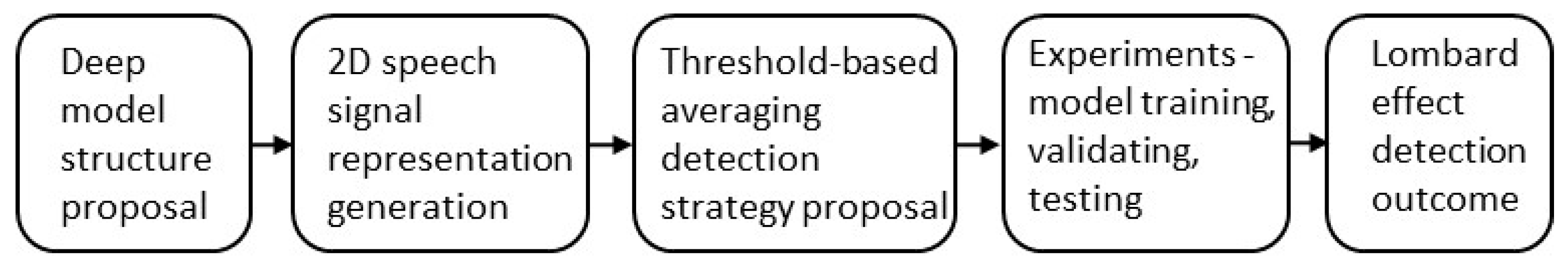
2. Lombard Speech Detection Process
2.1. Deep Model Structure
- -
- Size of the filter tensor (it is usually two- or three-dimensional since the image might be greyscale or color);
- -
- Stride—the number of pixels by which the filter is moved in the subsequent steps;
- -
- Padding—whether the resulting pixel set should be padded with empty pixels to retain the exact size of the feature map as the source image;
- -
- The number of filters that should be applied to the image.
2.2. 2D Speech Signal Representation
- (1)
- Spectrogram
- (2)
- Mel spectrogram
- (3)
- Chromagram
- (4)
- MFCC-gram
2.3. Threshold-Based Strategy of Averaging the Lombard Effect Detection Result
| Algorithm 1: A procedure for averaging the Lombard effect detection results. |
| INPUT: vector If then the frame is non-Lombard else the frame is Lombard-like end if OUTPUT: the value of |
- -
- It was assumed that the threshold for classifying a given frame as Lombard is 0.5, i.e., if the neural network returns the vector for each frame, it returns two probabilities: probability , when the given frame is neutral speech; probability , in the case of Lombard speech.
- -
- For , neutral speech, for , Lombard speech.
3. Experiments and Result Analysis
3.1. Experimental Setup
3.2. Preparation of Recordings
3.3. Results
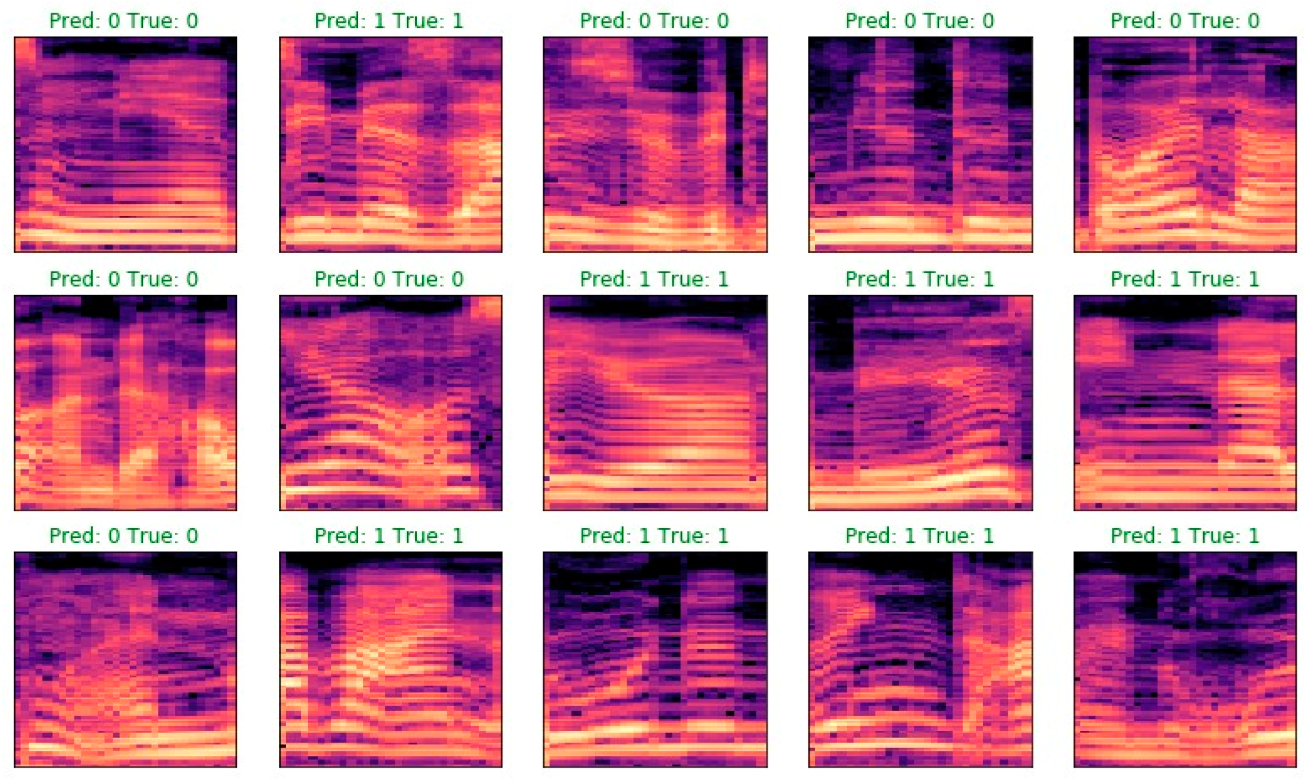
3.3.1. Effectiveness of 2D Feature Representations Combined with CNN for Lombard Speech Detection
- -
- Conv2D is a basic two-dimensional convolutional layer (a two-dimensional convolutional layer means that the input matrix is three-dimensional, representing width, height, and the number of filters).
- -
- Max_pooling2D is a max-pooling layer, reducing the dimensions of the input layer.
- -
- Dropout is an operation of randomly ignoring selected neurons in the learning process; this is a method of regularization and thus improves the results of learning in terms of the ability to generalize.
- -
- Flatten is a flattening operation which means that the three-dimensional output matrix is flattened into a vector that can be used in the typical dense layer.
- -
- Dense is a basic neural network flat layer.
- -
- The experiments are numbered from one to nine and are presented below.
- -
- Gender of the speaker;
- -
- F0 frequency;
- -
- First two MFCCs.
- -
- Every speech recording was resampled using 22,050 Hz frequency;
- -
- Average F0 was calculated for the whole file;
- -
- Average MFCCs were calculated (second and third coefficient).
3.3.2. Evaluation of the Lombard Speech Detection Process Effectiveness
- -
- G1 model—a network trained on the German dataset in a proportion of 2/3 (including 7% of recordings for validation). Recordings are split into training, validation, and test sets.
- -
- G2 model—a network trained on the German dataset of six speakers and tested on the other two speakers.
- -
- P1 model—a network trained on the Polish dataset in a proportion of 2/3 (including 7% of recordings for validation). Recordings are split into training, validation, and test sets.
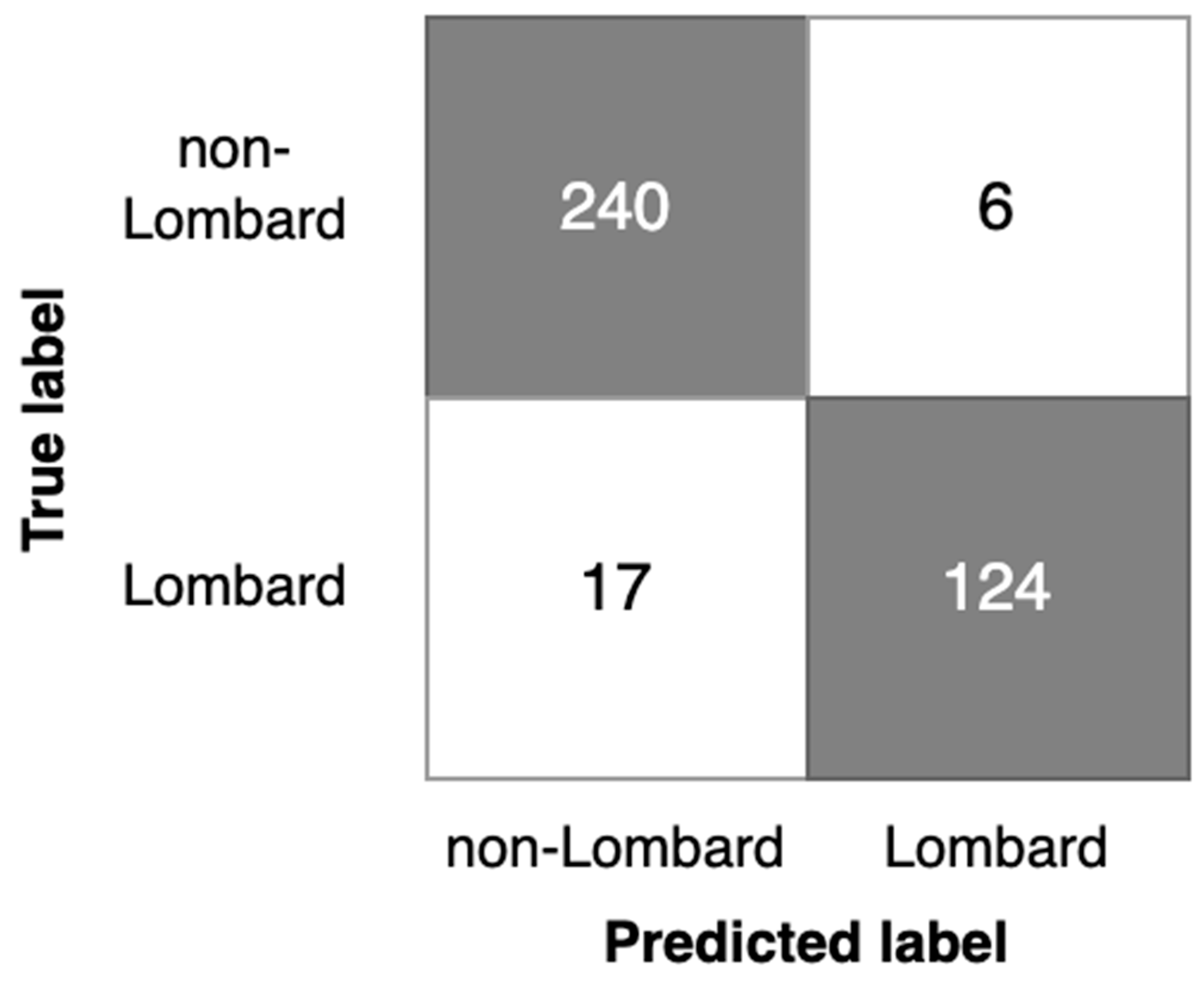
3.3.3. Discussion
- -
- Analysis of detection errors (Figure 8, Figure 9 and Figure 10) shows the predominance of false negative errors (i.e., Lombard speech was identified as non-Lombard). The error rate was 1.6–3 times higher than the rate of false positive type errors (non-Lombard speech was detected as Lombard). This may be due to the highly specific characteristics of some speakers or the insufficient discriminant power of augmented features. In the latter case, the study of 2D representation augmentation should be continued in the search for additional features.
- -
- The investigated setup enabled the near real-time detection of the Lombard effect. An operational delay of 0.5–0.7 s was found during the investigation, which is acceptable for real-world applications.
- -
- Gender information should be used to identify the Lombard speech. Therefore, it is necessary to consider an automated gender identification stage, preferably using a separate classification model. Our experimental results show 93% accuracy of spectrogram-based speaker gender identification (Experiment 1), which may be sufficient for Lombard speech identification.
- -
- The detection process should also consider the silence between utterances and be capable of disregarding these fragments. Possible solutions for deployment are as follows: the Lombard speech identification process may be extended to a three-valued classification, i.e., non-Lombard speech, Lombard speech, or a voice activity detection (VAD) algorithm should be used separately as a self-sufficient component supporting silence detection.
- -
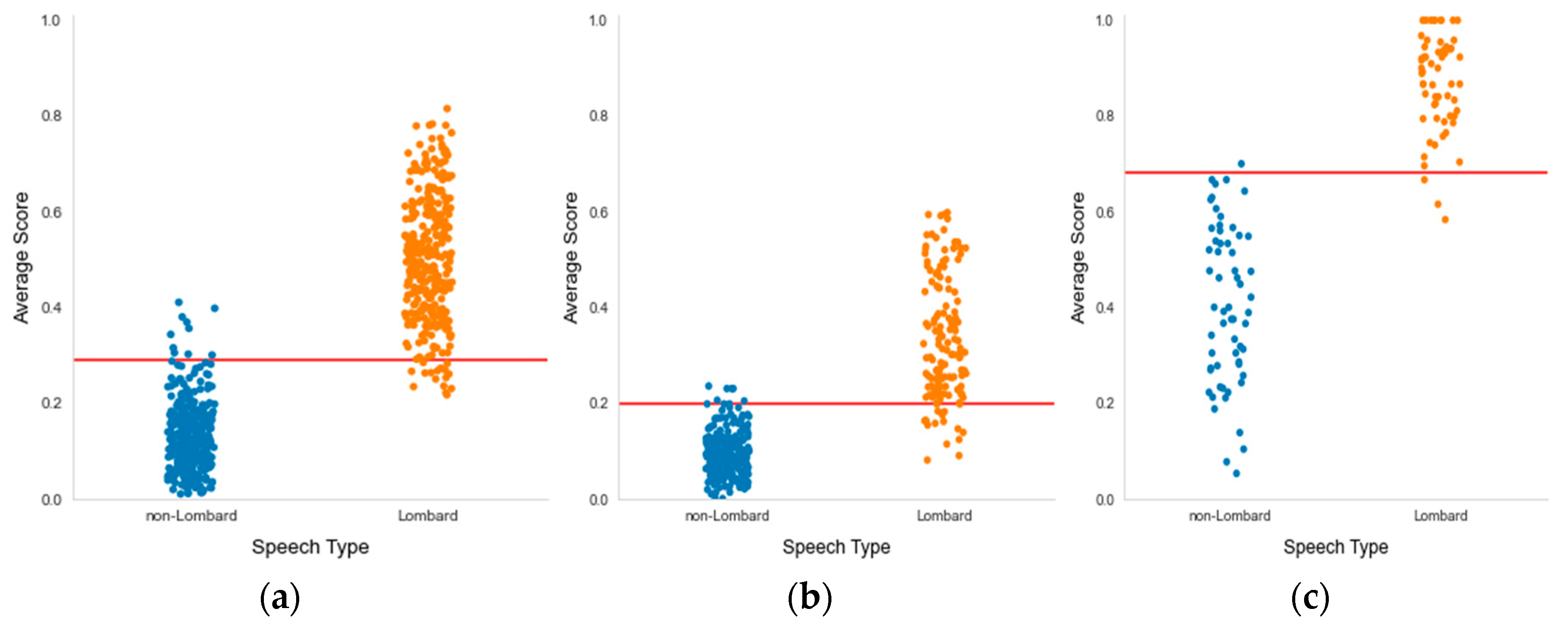
- The implemented Lombard speech detection setup requires defining the cutoff value between Lombard and non-Lombard speech. These values differ for different datasets (Figure 11). The automatic definition of this value is one of the challenges for future research.
4. Conclusions
Author Contributions
Funding
Institutional Review Board Statement
Informed Consent Statement
Data Availability Statement
Conflicts of Interest
References
- Lombard, E. Le signe de l’elevation de la voix. Ann. Mal. De L’Oreille Et Du Larynx 1911, 37, 101–119. [Google Scholar]
- Junqua, J.-C. The influence of acoustics on speech production: A noise-induced stress phenomenon known as the Lombard reflex. Speech Commun. 1996, 20, 13–22. [Google Scholar] [CrossRef]
- Amazi, D.K.; Garber, S.R. The Lombard sign as a function of age and task. J. Speech Lang. Hear. Res. 1982, 25, 581–585. [Google Scholar] [CrossRef] [PubMed]
- Khan, M.N.; Naseer, F. IoT based university garbage monitoring system for healthy environment for students. In Proceedings of the 14th International Conference on Semantic Computing (ICSC), San Diego, CA, USA, 3–5 February 2020; IEEE: Manhattan, NY, USA, 2020; pp. 354–358. [Google Scholar]
- Jamil, M.; Khan, M.N.; Rind, S.J.; Awais, Q.; Uzair, M. Neural network predictive control of vibrations in tall structure: An experimental controlled vision. Comput. Electr. Eng. 2021, 89, 106940. [Google Scholar] [CrossRef]
- Justus, D.; Brennan, J.; Bonner, S.; McGough, A.S. Predicting the computational cost of deep learning models. In Proceedings of the 2018 IEEE International Conference on Big Data (Big Data), Seattle, WA, USA, 10–13 December 2018; pp. 3873–3882. [Google Scholar]
- Lopez-Ballester, J.; Pastor-Aparicio, A.; Felici-Castell, S.; Segura-Garcia, J.; Cobos, M. Enabling real-time computation of psycho-acoustic parameters in acoustic sensors using convolutional neural networks. IEEE Sens. J. 2020, 20, 11429–11438. [Google Scholar] [CrossRef]
- He, Y.; Dong, X. Real time speech recognition algorithm on embedded system based on continuous Markov model. Microprocess. Microsyst. 2020, 75, 103058. [Google Scholar] [CrossRef]
- Phruksahiran, N. Audio Feature and Correlation Function-Based Speech Recognition in FM Radio Broadcasting. ECTI Transactions on Electrical Engineering, Electron. Commun. 2022, 20, 403–413. [Google Scholar] [CrossRef]
- Bottalico, P.; Piper, R.N.; Legner, B. Lombard effect, intelligibility, ambient noise, and willingness to spend time and money in a restaurant amongst older adults. Sci. Rep. 2022, 12, 6549. [Google Scholar] [CrossRef]
- Hansen, J.H.; Lee, J.; Ali, H.; Saba, J.N. A speech perturbation strategy based on “Lombard effect” for enhanced intelligibility for cochlear implant listeners. J. Acoust. Soc. Am. 2020, 147, 1418–1428. [Google Scholar] [CrossRef]
- Ngo, T.; Kubo, R.; Akagi, M. Increasing speech intelligibility and naturalness in noise based on concepts of modulation spectrum and modulation transfer function. Speech Commun. 2021, 135, 11–24. [Google Scholar] [CrossRef]
- Boril, H.; Hansen, J.H. Unsupervised equalization of Lombard effect for speech recognition in noisy adverse environments. IEEE Trans. Audio Speech Lang. Process. 2009, 18, 1379–1393. [Google Scholar] [CrossRef]
- Heracleous, P.; Ishi, C.T.; Sato, M.; Ishiguro, H.; Hagita, N. Analysis of the visual Lombard effect and automatic recognition experiments. Comput. Speech Lang. 2013, 27, 288–300. [Google Scholar] [CrossRef]
- Marxer, R.; Barker, J.; Alghamdi, N.; Maddock, S. The impact of the Lombard effect on audio and visual speech recognition systems. Speech Commun. 2018, 100, 58–68. [Google Scholar] [CrossRef]
- Vlaj, D.; Kacic, Z. The influence of Lombard effect on speech recognition. In Speech Technologies; IntechOpen: London, UK, 2011; pp. 1998–2001. [Google Scholar]
- Kelly, F.; Hansen, J.H. Evaluation and calibration of Lombard effects in speaker verification. In Proceedings of the 2016 IEEE Spoken Language Technology Workshop (SLT), San Diego, CA, USA, 13–16 December 2016; pp. 205–209. [Google Scholar]
- Kelly, F.; Hansen, J.H. Analysis and calibration of Lombard effect and whisper for speaker recognition. IEEE/ACM Trans. Audio Speech Lang. Process. 2021, 29, 927–942. [Google Scholar] [CrossRef] [PubMed]
- Saleem, M.M.; Liu, G.; Hansen, J.H. Weighted training for speech under Lombard effect for speaker recognition. In Proceedings of the 40th IEEE International Conference on Acoustics, Speech and Signal Processing (ICASSP), Brisbane, QLD, Australia, 19–24 April 2015; pp. 4350–4354. [Google Scholar]
- Zhao, Y.; Ando, A.; Takaki, S.; Yamagishi, J.; Kobashikawa, S. Does the Lombard Effect Improve Emotional Communication in Noise?-Analysis of Emotional Speech Acted in Noise. In Proceedings of the INTERSPEECH. Graz, Austria, 15–19 September 2019; pp. 3292–3296. [Google Scholar]
- Junqua, J.-C. The Lombard reflex and its role on human listeners and automatic speech recognizers. J. Acoust. Soc. Am. 1993, 93, 510–524. [Google Scholar] [CrossRef]
- Kisic, D.; Horvat, M.; Jambrošic, K.; Francek, P. The Potential of Speech as the Calibration Sound for Level Calibration of Non-Laboratory Listening Test Setups. Appl. Sci. 2022, 12, 7202. [Google Scholar] [CrossRef]
- Ma, P.; Petridis, S.; Pantic, M. Investigating the Lombard effect influence on end-to-end audio-visual speech recognition. In Proceedings of the Interspeech, Graz, Austria, 15–19 September 2019; pp. 4090–4094. [Google Scholar] [CrossRef]
- Steeneken, H.J.M.; Hansen, J.H.L. Speech under stress conditions: Overview of the effect on the speech production and on system performance. In Proceedings of the IEEE International Conference on Acoustics, Speech, and Signal Processing Proceedings (ICASSP99), Phoenix, AZ, USA, 15–19 March 1999; Volume 4, pp. 2079–2082. [Google Scholar]
- Kurowski, A.; Kotus, J.; Odya, P.; Kostek, B. A Novel Method for Intelligibility Assessment of Nonlinearly Processed Speech in Spaces Characterized by Long Reverberation Times. Sensors 2022, 22, 1641. [Google Scholar] [CrossRef]
- Cooke, M.; Lecumberri, M.L.G. The intelligibility of Lombard speech for non-native listeners. J. Acoust. Soc. Am. 2012, 132, 1120–1129. [Google Scholar] [CrossRef]
- Marcoux, K.; Cooke, M.; Tucker, B.V.; Ernestus, M. The Lombard intelligibility benefit of native and non-native speech for native and non-native listeners. Speech Commun. 2022, 136, 53–62. [Google Scholar] [CrossRef]
- Summers, W.V.; Pisoni, D.B.; Bernacki, R.H.; Pedlow, R.I.; Stokes, M.A. Effects of noise on speech production: Acoustic and perceptual analyses. J. Acoust. Soc. Am. 1988, 84, 917–928. [Google Scholar] [CrossRef]
- Trabelsi, A.; Warichet, S.; Aajaoun, Y.; Soussilane, S. Evaluation of the efficiency of state-of-the-art Speech Recognition engines. Procedia Comput. Sci. 2022, 207, 2242–2252. [Google Scholar] [CrossRef]
- Abdusalomov, A.B.; Safarov, F.; Rakhimov, M.; Turaev, B.; Whangbo, T.K. Improved Feature Parameter Extraction from Speech Signals Using Machine Learning Algorithm. Sensors 2022, 22, 8122. [Google Scholar] [CrossRef] [PubMed]
- Ogundokun, R.O.; Abikoye, O.C.; Adegun, A.A.; Awotunde, J.B. Speech Recognition System: Overview of the State-Of-The-Arts. Int. J. Eng. Res. Technol. 2020, 13, 384–392. [Google Scholar] [CrossRef]
- Hannun, A.; Case, C.; Casper, J.; Catanzaro, B.; Diamos, G.; Elsen, E.; Prenger, R.; Satheesh, S.; Sengupta, S.; Coates, A.; et al. Deep speech: Scaling up end-to-end speech recognition. arXiv 2014, arXiv:1412.5567. [Google Scholar]
- Povey, D.; Ghoshal, A.; Boulianne, G.; Burget, L.; Glembek, O.; Goel, N.; Hannemann, M.; Motlicek, P.; Qian, Y.; Schwarz, P.; et al. The kaldi speech recognition toolkit. In Proceedings of the IEEE 2011 Workshop on Automatic Speech Recognition and Understanding, Big Island, HI, USA, 11–15 December 2011. [Google Scholar]
- Che, G.; Chai, S.; Wang, G.-B.; Du, J.; Zhang, W.-Q.; Weng, C.; Su, D.; Povey, D.; Trmal, J.; Zhang, J.; et al. GigaSpeech: An Evolving, Multi-Domain ASR Corpus with 10,000 Hours of Transcribed Audio. In Proceedings of the INTERSPEECH 2021, Brno, Czechia, 30 August–3 September 2021; pp. 3670–3674. [Google Scholar] [CrossRef]
- Ezzerg, A.; Gabrys, A.; Putrycz, B.; Korzekwa, D.; Trigueros, D.S.; McHardy, D.; Pokora, K.; Lachowicz, J.; Trueba, J.L.; Klimkov, V. Enhancing Audio Quality for Expressive Neural Text-to-Speech. arXiv 2021, arXiv:2108.06270. [Google Scholar]
- Jiao, Y.; Gabryś, A.; Tinchev, G.; Putrycz, B.; Korzekwa, D.; Klimkov, V. Universal neural vocoding with parallel wavenet. In Proceedings of the ICASSP 2021 IEEE International Conference on Acoustics, Speech and Signal Processing (ICASSP), Toronto, ON, Canada, 6–11 June 2021; pp. 6044–6048. [Google Scholar]
- Merritt, T.; Ezzerg, A.; Biliński, P.; Proszewska, M.; Pokora, K.; Barra-Chicote, R.; Korzekwa, D. Text-Free Non-Parallel Many-to-Many Voice Conversion Using Normalising Flows. arXiv 2022, arXiv:2203.08009. [Google Scholar]
- Nossier, S.A.; Wall, J.; Moniri, M.; Glackin, C.; Cannings, N. An Experimental Analysis of Deep Learning Architectures for Supervised Speech Enhancement. Electronics 2021, 10, 17. [Google Scholar] [CrossRef]
- Korvel, G.; Kąkol, K.; Kurasova, O.; Kostek, B. Evaluation of Lombard speech models in the context of speech in noise enhancement. IEEE Access 2020, 8, 155156–155170. [Google Scholar] [CrossRef]
- Zhang, J.; Zorila, C.; Doddipatla, R.; Barker, J. On Monoaural Speech Enhancement for Automatic Recognition of Real Noisy Speech Using Mixture Invariant Training. arXiv 2022, arXiv:2205.01751. [Google Scholar]
- Furoh, T.; Fukumori, T.; Nakayama, M.; Nishiura, T. Detection for Lombard speech with second-order mel-frequency cepstral coefficient and spectral envelope in beginning of talking-speech. In Proceedings of the Meetings on Acoustics ICA2013), Montreal, QC, Canada, 2–7 June 2013; Acoustical Society of America: Melville, NY, USA, 2013; Volume 19, p. 060013. [Google Scholar]
- Goyal, J.; Khandnor, P.; Aseri, T.C. Classification, prediction, and monitoring of Parkinson’s disease using computer assisted technologies: A comparative analysis. Eng. Appl. Artif. Intell. 2020, 96, 103955. [Google Scholar] [CrossRef]
- Scharf, M.K.; Hochmuth, S.; Wong, L.L.; Kollmeier, B.; Warzybok, A. Lombard Effect for Bilingual Speakers in Cantonese and English: Importance of Spectro-Temporal Features. arXiv 2022, arXiv:2204.06907. [Google Scholar]
- Piotrowska, M.; Korvel, G.; Kostek, B.; Ciszewski, T.; Czyzewski, A. Machine learning-based analysis of English lateral allophones. Int. J. Appl. Math. Comput. Sci. 2019, 29, 393–405. [Google Scholar] [CrossRef]
- Piotrowska, M.; Czyzewski, A.; Ciszewski, T.; Korvel, G.; Kurowski, A.; Kostek, B. Evaluation of aspiration problems in L2 English pronunciation employing machine learning. J. Acoust. Soc. Am. 2021, 150, 120–132. [Google Scholar] [CrossRef]
- Korvel, G.; Treigys, P.; Tamulevicius, G.; Bernataviciene, J.; Kostek, B. Analysis of 2D Feature Spaces for Deep Learning-Based Speech Recognition. J. Audio Eng. Soc. 2018, 66, 1072–1081. [Google Scholar] [CrossRef]
- Vafeiadis, A.; Votis, K.; Giakoumis, D.; Tzovaras, D.; Chen, L.; Hamzaoui, R. Audio content analysis for unobtrusive event detection in smart homes. Eng. Appl. Artif. Intell. 2020, 89, 103226. [Google Scholar] [CrossRef]
- Tamulevičius, G.; Korvel, G.; Yayak, A.B.; Treigys, P.; Bernatavičienė, J.; Kostek, B. A study of cross-linguistic speech emotion recognition based on 2D feature spaces. Electronics 2020, 9, 1725. [Google Scholar] [CrossRef]
- Tariq, Z.; Shah, S.K.; Lee, Y. Speech Emotion Detection using IoT based Deep Learning for Health Care. In Proceedings of the IEEE International Conference on Big Data (Big Data), Los Angeles, CA, USA, 9–12 December 2019; pp. 4191–4196. [Google Scholar] [CrossRef]
- Er, M.B.; Isik, E.; Isik, I. Parkinson’s detection based on combined CNN and LSTM using enhanced speech signals with variational mode decomposition. Biomed. Signal Process. Control. 2021, 70, 103006. [Google Scholar] [CrossRef]
- Almeida, J.S.; Rebouças Filho, P.P.; Carneiro, T.; Wei, W.; Damaševičius, R.; Maskeliūnas, R.; de Albuquerque, V.H.C. Detecting Parkinson’s disease with sustained phonation and speech signals using machine learning techniques. Pattern Recognit. Lett. 2019, 125, 55–62. [Google Scholar] [CrossRef]
- Laguarta, J.; Hueto, F.; Subirana, B. COVID-19 artificial intelligence diagnosis using only cough recordings. IEEE Open J. Eng. Med. Biol. 2020, 1, 275–281. [Google Scholar] [CrossRef]
- Gu, J.; Wang, Z.; Kuen, J.; Ma, L.; Shahroudy, A.; Shuai, B.; Liu, T.; Wang, X.; Wang, G.; Cai, J.; et al. Recent advances in convolutional neural networks. Pattern Recognit. 2018, 77, 354–377. [Google Scholar] [CrossRef]
- LeCun, Y.; Haffner, P.; Bottou, L.; Bengio, Y. Object Recognition with Gradient-Based Learning. In Shape, Contour and Grouping in Computer Vision; Lecture Notes in Computer Science (Including Subseries Lecture Notes in Artificial Intelligence and Lecture Notes in Bioinformatics); Springer: Berlin/Heidelberg, Germany, 1999; Volume 1681, pp. 319–345. [Google Scholar]
- Müller, M. Fundamentals of Music Processing: Audio, Analysis, Algorithms, Applications; Springer: New York, NY, USA; Cham, Switzerland, 2015. [Google Scholar]
- Soloducha, M.; Raake, A.; Kettler, F.; Voigt, P. Lombard speech database for German language. In Proceedings of the 42nd Annual Conference on Acoustics (DAGA), Aachen, Germany, 14–17 March 2016. [Google Scholar]
- Czyzewski, A.; Kostek, B.; Bratoszewski, P.; Kotus, J.; Szykulski, M. An audio-visual corpus for multimodal automatic speech recognition. J. Intell. Inf. Syst. 2017, 49, 167–192. [Google Scholar] [CrossRef]
- Park, D.S.; Chan, W.; Zhang, Y.; Chiu, C.-C.; Zoph, B.; Cubuk, E.D.; Le, Q.V. SpecAugment: A Simple Data Augmentation Method for Automatic Speech Recognition. In Proceedings of the Interspeech 2019, Graz, Austria, 15–19 September 2019; pp. 2613–2617. [Google Scholar]
- Song, X.; Wu, Z.; Huang, Y.; Su, D.; Meng, H. SpecSwap: A Simple Data Augmentation Method for End-to-End Speech Recognition. In Proceedings of the Interspeech 2020, Shanghai, China, 25–29 October 2020; pp. 581–585. [Google Scholar]
- Abayomi-Alli, O.O.; Damaševičius, R.; Qazi, A.; Adedoyin-Olowe, M.; Misra, S. Data Augmentation and Deep Learning Methods in Sound Classification: A Systematic Review. Electronics 2022, 11, 3795. [Google Scholar] [CrossRef]
- Junqua, J.C.; Fincke, S.; Field, K. The Lombard effect: A reflex to better communicate with others in noise. In Proceedings of the 1999 IEEE International Conference on Acoustics, Speech, and Signal Processing, ICASSP99 (Cat. No. 99CH36258), Phoenix, AZ, USA, 4 March 1999; Volume 4, pp. 2083–2086. [Google Scholar]
- Alghamdi, N.; Maddock, S.; Marxer, R.; Barker, J.; Brown, G.J. A corpus of audio-visual Lombard speech with frontal and profile views. J. Acoust. Soc. Am. 2018, 143, EL523–EL529. [Google Scholar] [CrossRef]
- Kleczkowski, P.; Żak, A.; Król-Nowak, A. Lombard effect in Polish speech and its comparison in English speech. Arch. Acoust. 2017, 42, 561–569. [Google Scholar] [CrossRef]
- Korzekwa, D.; Lorenzo-Trueba, J.; Drugman, T.; Kostek, B. Computer-assisted pronunciation training—Speech synthesis is almost all you need. Speech Commun. 2022, 142, 22–33. [Google Scholar] [CrossRef]


| Language | Set Details |
|---|---|
| German (Soloducha et al., 2016) [56] | 40 s-long statements 8 speakers (including 3 females and 5 males) Each sentence was recorded under conditions of silence and with accompanying disturbance |
| Polish (Czyzewski et al., 2017) [57] | 15 s-long statements 4 speakers (including 2 females and 2 males) Each sentence was recorded under conditions of silence and with accompanying disturbance. |
| Layer (Type) | Output Shape | Number of Parameters |
|---|---|---|
| conv2d_2 (Conv2D) | (None, 90, 93, 32) | 544 |
| max_pooling2d_2 (MaxPooling2D) | (None, 45, 46, 32) | 0 |
| dropout_3 (Dropout) | (None, 45, 46, 32) | 0 |
| conv2d_3 (Conv2D) | (None, 45, 46, 16) | 2064 |
| max_pooling2d_3 (MaxPooling2D) | (None, 22, 23, 16) | 0 |
| dropout_4 (Dropout) | (None, 22, 23, 16) | 0 |
| flatten_1 (Flatten) | (None, 8096) | 0 |
| dense_2 (Dense) | (None, 256) | 2,072,832 |
| dropout_5 (Dropout) | (None, 256) | 0 |
| dense_3 (Dense) | (None, 2) | 514 |
| Layer (Type) | Output Shape | Number of Parameters |
|---|---|---|
| conv2d_12 (Conv2D) | (None, 90, 93, 32) | 2080 |
| max_pooling2d_12 (MaxPooling2D) | (None, 45, 46, 32) | 0 |
| dropout_20 (Dropout) | (None, 45, 46, 32) | 0 |
| conv2d_13 (Conv2D) | (None, 45, 46, 48) | 24,624 |
| max_pooling2d_13 (MaxPooling2D) | (None, 22, 23, 48) | 0 |
| dropout_21 (Dropout) | (None, 22, 23, 48) | 0 |
| flatten_4 (Flatten) | (None, 24,288) | 0 |
| dense_12 (Dense) | (None, 256) | 6,217,984 |
| dropout_22 (Dropout) | (None, 256) | 0 |
| dense_13 (Dense) | (None, 2) | 514 |
| Layer (Type) | Output Shape | Number of Parameters |
|---|---|---|
| conv2d_14 (Conv2D) | (None, 90, 93, 32) | 1184 |
| max_pooling2d_14 (MaxPooling2D) | (None, 45, 46, 32) | 0 |
| dropout_23 (Dropout) | (None, 45, 46, 32) | 0 |
| conv2d_15 (Conv2D) | (None, 45, 46, 48) | 13,872 |
| max_pooling2d_15 (MaxPooling2D) | (None, 22, 23, 48) | 0 |
| dropout_24 (Dropout) | (None, 22, 23, 48) | 0 |
| conv2d_16 (Conv2D) | (None, 22, 23, 64) | 27,712 |
| max_pooling2d_16 (MaxPooling2D) | (None, 11, 11, 64) | 0 |
| dropout_25 (Dropout) | (None, 11, 11, 64) | 0 |
| flatten_5 (Flatten) | (None, 7744) | 0 |
| dense_14 (Dense) | (None, 256) | 1,982,720 |
| dropout_26 (Dropout) | (None, 256) | 0 |
| dense_15 (Dense) | (None, 2) | 514 |
| ID | Model According to Table 3 (1st Model) and Table 4 (2nd Model) | Number of Filters in Conv. Layers | Size of Kernel | Max Pooling | Dropout after Conv. Layers | Dropout after Dense Layer | Number of Neurons in the Dense Layer | Batch Size | Number of Epochs |
|---|---|---|---|---|---|---|---|---|---|
| 1 | 1 | 16, 32 | 2 | 2 | 0.3 | 0.5 | 256 | 64 | 35 |
| 2 | 1 | 32, 48 | 2 | 2 | 0.3 | 0.5 | 256 | 64 | 35 |
| 3 | 1 | 32, 48 | 3 | 2 | 0.3 | 0.5 | 256 | 64 | 35 |
| 4 | 1 | 32, 48 | 3 | 2 | 0.3 | 0.5 | 256 | 32 | 35 |
| 5 | 1 | 32, 48 | 5 | 2 | 0.3 | 0.5 | 256 | 64 | 35 |
| 6 | 1 | 32, 48 | 5 | 2 | 0.3 | 0.5 | 256 | 32 | 35 |
| 7 | 2 | 32, 48, 64 | 3 | 2 | 0.3 | 0.5 | 256 | 64 | 35 |
| 8 | 2 | 32, 48, 64 | 5 | 3 | 0.3 | 0.5 | 256 | 64 | 35 |
| 9 | 2 | 32, 48, 64 | 5 | 3 | 0.3 | 0.5 | 256 | 32 | 35 |
| Result No. | Type of Graphical Representation Employed | Augmented/Clean Picture | Experiment Configuration According to ID from Table 5 | Accuracy of the Testing Set |
|---|---|---|---|---|
| 1 | Mel spectrogram | Augmented | 9 | 0.8671875 |
| 2 | Spectrogram | Clean | 8 | 0.8515625 |
| 3 | Spectrogram | Clean | 6 | 0.84375 |
| 4 | Spectrogram | Clean | 4 | 0.8359375 |
| 5 | Spectrogram | Augmented | 8 | 0.828125 |
| 6 | Spectrogram | Augmented | 9 | 0.828125 |
| 7 | Spectrogram | Augmented | 7 | 0.8125 |
| 8 | Mel spectrogram | Clean | 6 | 0.8125 |
| 9 | Spectrogram | Clean | 7 | 0.8046875 |
| 10 | Spectrogram | Augmented | 5 | 0.8046875 |
| 11 | Mel spectrogram | Clean | 7 | 0.8046875 |
| 12 | Mel spectrogram | Augmented | 6 | 0.8046875 |
| 13 | Mel spectrogram | Clean | 5 | 0.796875 |
| 14 | Spectrogram | Clean | 5 | 0.7890625 |
| 15 | Mel spectrogram | Clean | 8 | 0.7890625 |
| Layer (Type) | Output Shape | Number of Parameters |
|---|---|---|
| conv2d_20 (Conv2D) | (None, 90, 93, 32) | 3232 |
| max_pooling2d_20 (MaxPooling2D) | (None, 30, 31, 32) | 0 |
| dropout_32 (Dropout) | (None, 30, 31, 32) | 0 |
| conv2d_21 (Conv2D) | (None, 30, 31, 48) | 38,448 |
| max_pooling2d_21 (MaxPooling2D) | (None, 10, 10, 48) | 0 |
| dropout_33 (Dropout) | (None, 10, 10, 48) | 0 |
| conv2d_22 (Conv2D) | (None, 10, 10, 64) | 76,864 |
| max_pooling2d_22 (MaxPooling2D) | (None, 3, 3, 64) | 0 |
| dropout_34 (Dropout) | (None, 3, 3, 64) | 0 |
| flatten_7 (Flatten) | (None, 576) | 0 |
| dense_19 (Dense) | (None, 512) | 295,424 |
| dropout_35 (Dropout) | (None, 512) | 0 |
| dense_20 (Dense) | (None, 256) | 131,328 |
| dropout_36 (Dropout) | (None, 256) | 0 |
| dense_21 (Dense) | (None, 2) | 514 |
| Model | G1 | G2 | P1 |
|---|---|---|---|
| Number of samples used for training | 3156 | 2334 | 816 |
| Number of samples used for validation | 790 | 584 | 205 |
| Accuracy of the validation set | 0.9899 | 0.9880 | 0.9902 |
| Loss of the validation set | 0.0370 | 0.0434 | 0.0432 |
| Cutoff level | 0.29 | 0.20 | 0.68 |
| Recognition accuracy | 0.9594 | 0.9406 | 0.9667 |
| Precision | 0.9681 | 0.9538 | 0.9828 |
| Recall | 0.9500 | 0.8794 | 0.9500 |
Disclaimer/Publisher’s Note: The statements, opinions and data contained in all publications are solely those of the individual author(s) and contributor(s) and not of MDPI and/or the editor(s). MDPI and/or the editor(s) disclaim responsibility for any injury to people or property resulting from any ideas, methods, instructions or products referred to in the content. |
© 2022 by the authors. Licensee MDPI, Basel, Switzerland. This article is an open access article distributed under the terms and conditions of the Creative Commons Attribution (CC BY) license (https://creativecommons.org/licenses/by/4.0/).
Share and Cite
Kąkol, K.; Korvel, G.; Tamulevičius, G.; Kostek, B. Detecting Lombard Speech Using Deep Learning Approach. Sensors 2023, 23, 315. https://doi.org/10.3390/s23010315
Kąkol K, Korvel G, Tamulevičius G, Kostek B. Detecting Lombard Speech Using Deep Learning Approach. Sensors. 2023; 23(1):315. https://doi.org/10.3390/s23010315
Chicago/Turabian StyleKąkol, Krzysztof, Gražina Korvel, Gintautas Tamulevičius, and Bożena Kostek. 2023. "Detecting Lombard Speech Using Deep Learning Approach" Sensors 23, no. 1: 315. https://doi.org/10.3390/s23010315
APA StyleKąkol, K., Korvel, G., Tamulevičius, G., & Kostek, B. (2023). Detecting Lombard Speech Using Deep Learning Approach. Sensors, 23(1), 315. https://doi.org/10.3390/s23010315