
Terahertz Nondestructive Testing with Ultra-Wideband FMCW Radar
 ,
,  , ,
, ,  and
and
Abstract
1. Introduction
2. FMCW Radar Design and Integration
2.1. Architecture
2.2. Performance and Characterization
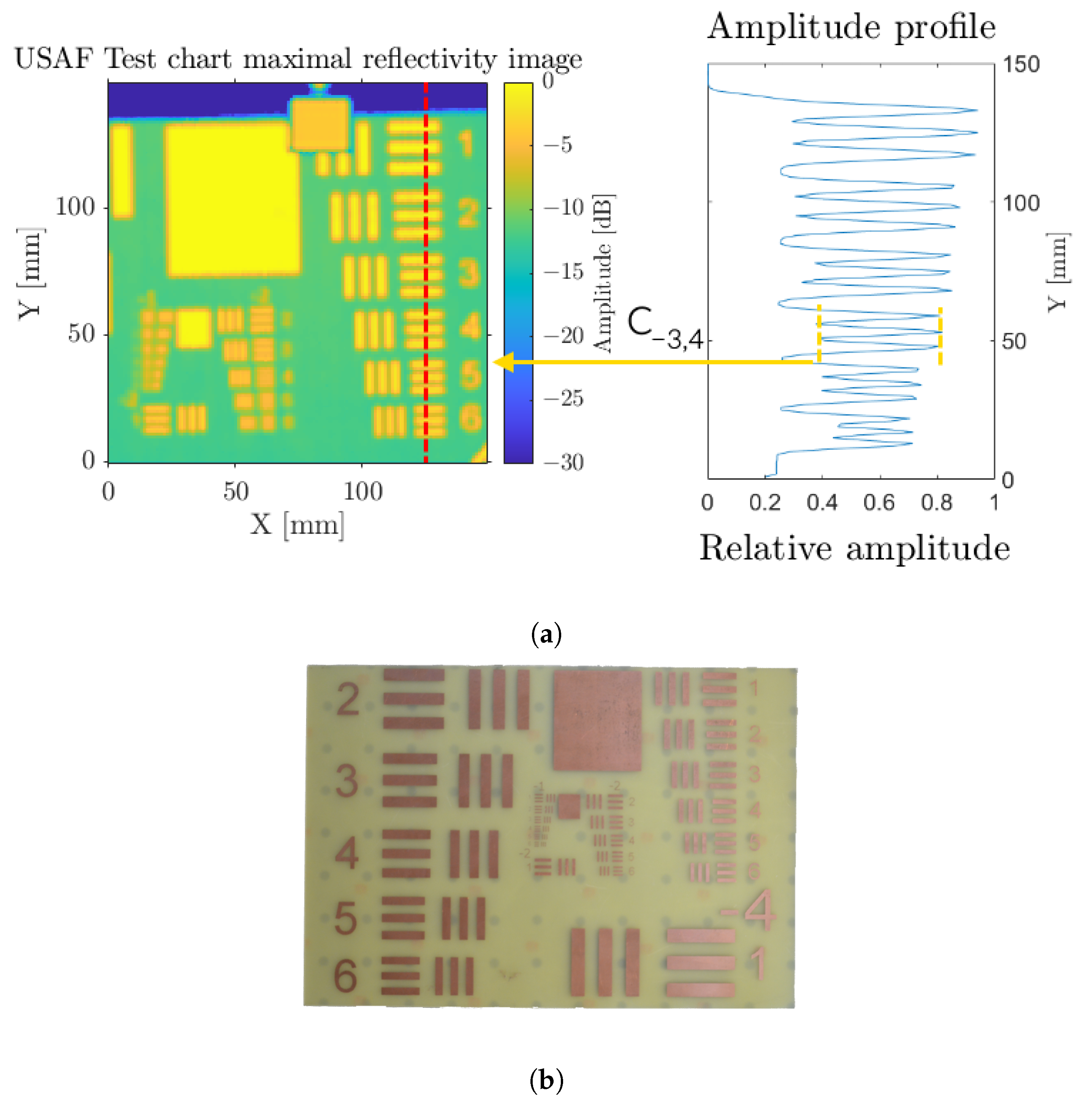
2.2.1. Lateral and Longitudinal Resolutions
Lateral Resolution
Longitudinal Resolution
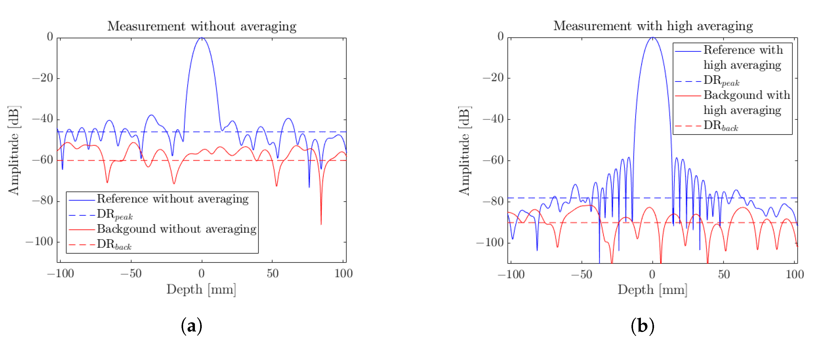
2.2.2. Dynamic Range
2.2.3. Stability
2.2.4. Longitudinal Sensing Precision and Accuracy
Longitudinal Precision
Longitudinal Accuracy
3. FMCW Imaging
3.1. Polymer Injected Sample Monitoring
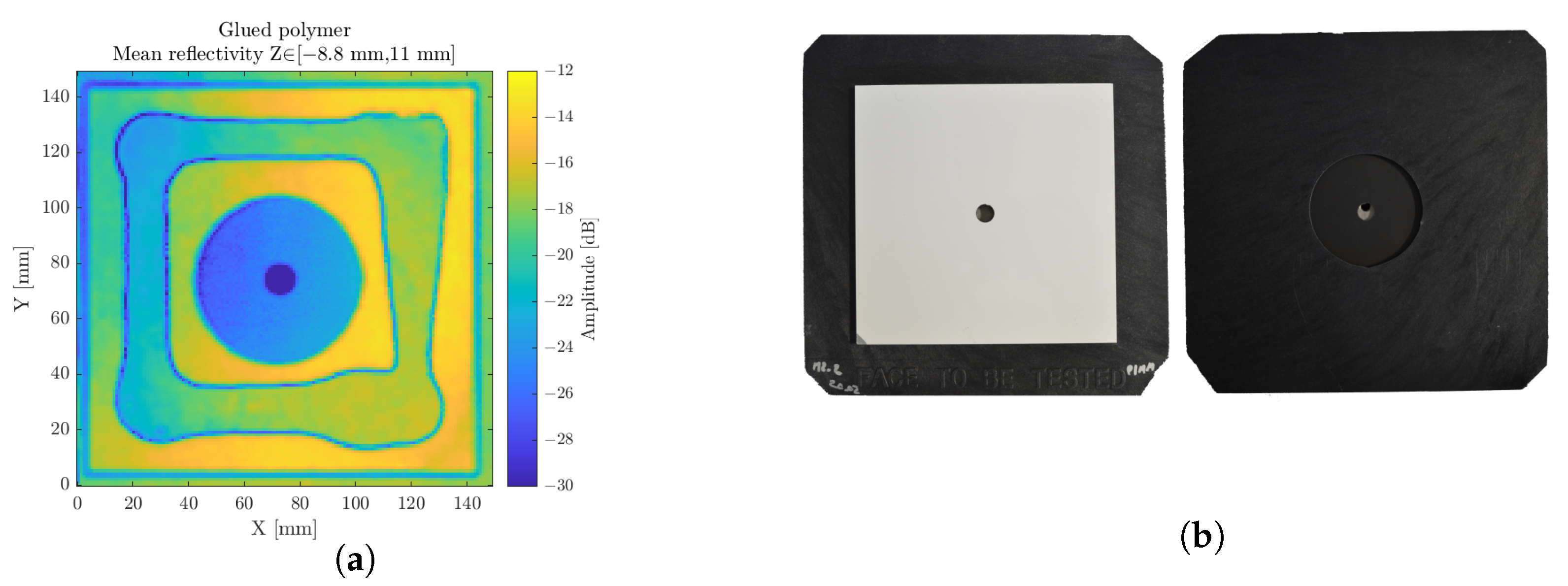
3.2. Polymer Gluing
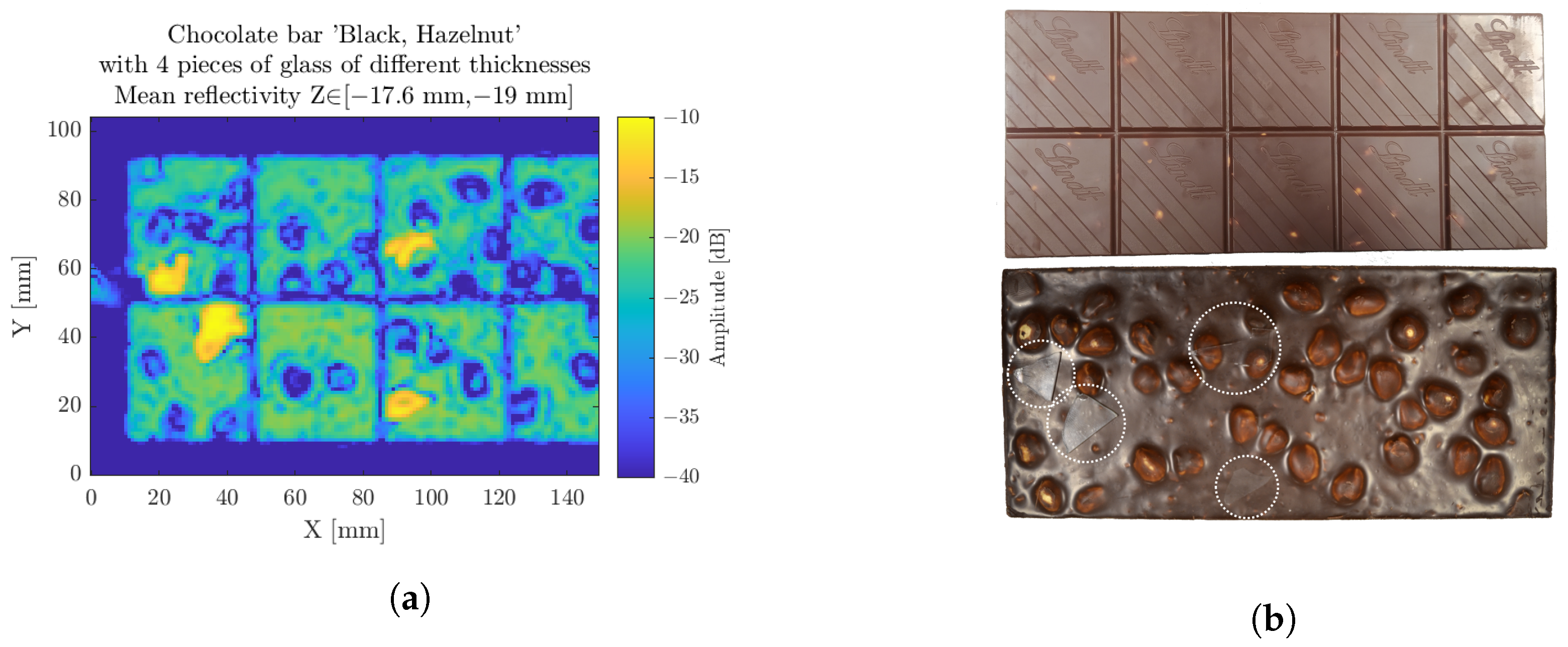
3.3. Chocolate Bar
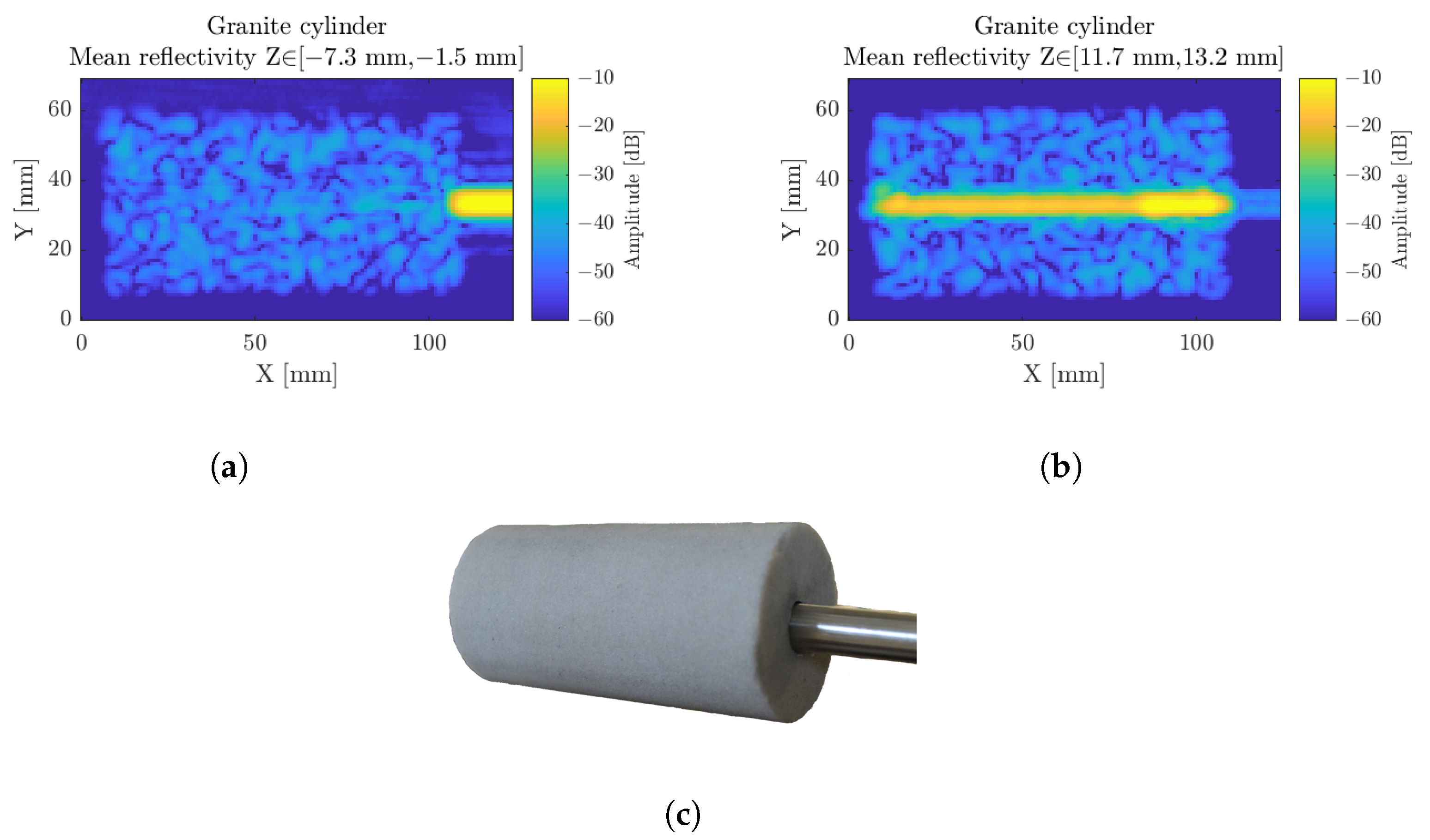
3.4. Crushed Granite Cylinder
3.5. Pharmaceutical Packaging Assessment
4. Conclusions
Author Contributions
Funding
Institutional Review Board Statement
Informed Consent Statement
Data Availability Statement
Conflicts of Interest
Abbreviations
| MDPI | Multidisciplinary Digital Publishing Institute |
| DOAJ | Directory of Open-Access Journals |
| FMCW | Frequency-modulated continuous wave |
| UWB | Ultra-wideband |
| NDT | Nondestructive testing |
| CW | Continuous wave |
| QCW | Quasi-continuous wave |
| LO | Local oscillator |
| HF | High frequency |
| IF | Intermediate frequency |
| VCO | Voltage-controlled oscillator |
| PLL | Phase-locked loop |
| SMA | Sub-Miniature Version A |
| DR | Dynamic range |
| SNR | Signal-to-noise ratio |
| SAR | Synthetic aperture radar |
| RMS | Root mean square |
| NA | Numerical aperture |
References
- Nüßler, D.; Jonuscheit, J. Terahertz based non-destructive testing (NDT). Tm-Tech. Mess. 2021, 88, 199–210. [Google Scholar] [CrossRef]
- Friederich, F.; Von Spiegel, W.; Bauer, M.; Meng, F.; Thomson, M.D.; Boppel, S.; Lisauskas, A.; Hils, B.; Krozer, V.; Keil, A.; et al. THz active imaging systems with real-time capabilities. IEEE Trans. Terahertz Sci. Technol. 2011, 1, 183–200. [Google Scholar] [CrossRef]
- Guillet, J.P.; Roux, M.; Wang, K.; Ma, X.; Fauquet, F.; Balacey, H.; Recur, B.; Darracq, F.; Mounaix, P. Art painting diagnostic before restoration with terahertz and millimeter waves. J. Infrared Millim. Terahertz Waves 2017, 38, 369–379. [Google Scholar] [CrossRef]
- Dandolo, C.L.K.; Guillet, J.P.; Ma, X.; Fauquet, F.; Roux, M.; Mounaix, P. Terahertz frequency modulated continuous wave imaging advanced data processing for art painting analysis. Opt. Express 2018, 26, 5358–5367. [Google Scholar] [CrossRef]
- Chopard, A.; Cassar, Q.; Bou-Sleiman, J.; Guillet, J.P.; Pan, M.; Perraud, J.; Susset, A.; Mounaix, P. Terahertz waves for contactless control and imaging in aeronautics industry. NDT E Int. 2021, 122, 102473. [Google Scholar] [CrossRef]
- Friederich, F.; May, K.H.; Baccouche, B.; Matheis, C.; Bauer, M.; Jonuscheit, J.; Moor, M.; Denman, D.; Bramble, J.; Savage, N. Terahertz radome inspection. Photonics 2018, 5, 1. [Google Scholar] [CrossRef]
- Taylor, J.D. Advanced Ultrawideband Radar: Signals, Targets, and Applications; CRC Press: Boca Raton, FL, USA, 2016. [Google Scholar]
- Lytid SAS. Available online: https://lytid.com/ (accessed on 17 November 2022).
- DOTNAC Project. Available online: https://cordis.europa.eu/docs/results/266320/final1-final-report-dotnac.pdf (accessed on 17 November 2022).
- Georges, M.; Zhao, Y. Imagerie Terahertz pour l’inspection des composites. In La Spectroscopie/Imagerie Térahertz: Un Nouvel Outil de Contrôle non Destructif; University of Liège: Liège, Belgium, 2018. [Google Scholar]
- Ellrich, F.; Bauer, M.; Schreiner, N.; Keil, A.; Pfeiffer, T.; Klier, J.; Weber, S.; Jonuscheit, J.; Friederich, F.; Molter, D. Terahertz quality inspection for automotive and aviation industries. J. Infrared, Millim. Terahertz Waves 2020, 41, 470–489. [Google Scholar] [CrossRef]
- Detlefsen, J.; Dallinger, A.; Schelkshorn, S.; Bertl, S. UWB millimeter-wave FMCW radar using hubert transform methods. In Proceedings of the 2006 IEEE Ninth International Symposium on Spread Spectrum Techniques and Applications, Manaus, Brazil, 28–31 August 2006; pp. 46–48. [Google Scholar]
- Nuttall, A. Some windows with very good sidelobe behavior. IEEE Trans. Acoust. Speech Signal Process. 1981, 29, 84–91. [Google Scholar] [CrossRef]
- Cristofani, E.; Friederich, F.; Wohnsiedler, S.; Matheis, C.; Jonuscheit, J.; Vandewal, M.; Beigang, R. Nondestructive testing potential evaluation of a terahertz frequency-modulated continuous-wave imager for composite materials inspection. Opt. Eng. 2014, 53, 031211. [Google Scholar] [CrossRef]
- Cooper, K.B.; Dengler, R.J.; Llombart, N.; Thomas, B.; Chattopadhyay, G.; Siegel, P.H. THz imaging radar for standoff personnel screening. IEEE Trans. Terahertz Sci. Technol. 2011, 1, 169–182. [Google Scholar] [CrossRef]
- Robertson, D.A.; Macfarlane, D.G.; Bryllert, T. 220 GHz wideband 3D imaging radar for concealed object detection technology development and phenomenology studies. In Proceedings of the Passive and Active Millimeter-Wave Imaging XIX, Baltimore, MD, USA, 17–21 April 2016; SPIE: Bellingham, WA, USA, 2016; Volume 9830, pp. 55–62. [Google Scholar]
- Pauli, M.; Göttel, B.; Scherr, S.; Bhutani, A.; Ayhan, S.; Winkler, W.; Zwick, T. Miniaturized millimeter-wave radar sensor for high-accuracy applications. IEEE Trans. Microw. Theory Tech. 2017, 65, 1707–1715. [Google Scholar] [CrossRef]
- Schmalz, K.; Winkler, W.; Borngraber, J.; Debski, W.; Heinemann, B.; Scheytt, C. A 122 GHz receiver in SiGe technology. In Proceedings of the 2009 IEEE Bipolar/BiCMOS Circuits and Technology Meeting, Capri, Italy, 12–14 October 2009; pp. 182–185. [Google Scholar]
- Schmalz, K.; Winkler, W.; Borngräber, J.; Debski, W.; Heinemann, B.; Scheytt, J. 122 GHz ISM-band transceiver concept and silicon ICs for low-cost receiver in SiGe BiCMOS. In Proceedings of the 2010 IEEE MTT-S International Microwave Symposium, Anaheim, CA, USA, 23–28 May 2010; pp. 1332–1335. [Google Scholar]
- Welp, B.; Hansen, S.; Briese, G.; Küppers, S.; Thomas, S.; Bredendiek, C.; Pohl, N. Versatile dual-receiver 94-GHz FMCW radar system with high output power and 26-GHz tuning range for high distance applications. IEEE Trans. Microw. Theory Tech. 2020, 68, 1195–1211. [Google Scholar] [CrossRef]
- Moreira, A.; Prats-Iraola, P.; Younis, M.; Krieger, G.; Hajnsek, I.; Papathanassiou, K.P. A tutorial on synthetic aperture radar. IEEE Geosci. Remote Sens. Mag. 2013, 1, 6–43. [Google Scholar] [CrossRef]
- Ding, J.; Kahl, M.; Loffeld, O.; Bolívar, P.H. THz 3-D image formation using SAR techniques: Simulation, processing and experimental results. IEEE Trans. Terahertz Sci. Technol. 2013, 3, 606–616. [Google Scholar] [CrossRef]
- Owens, J.C. Optical refractive index of air: Dependence on pressure, temperature and composition. Appl. Opt. 1967, 6, 51–59. [Google Scholar] [CrossRef] [PubMed]
- Wong, T.M.; Kahl, M.; Haring Bolívar, P.; Kolb, A. Computational image enhancement for frequency modulated continuous wave (FMCW) THz image. J. Infrared Millim. Terahertz Waves 2019, 40, 775–800. [Google Scholar] [CrossRef]
- Wong, T.M.; Kahl, M.; Bolıvar, P.H.; Kolb, A. Frequency modulated continuous wave (FMCW) THz image 3-D superresolution. arXiv 2018, arXiv:1802.05457. [Google Scholar]
- Ok, G.; Park, K.; Kim, H.J.; Chun, H.S.; Choi, S.W. High-speed terahertz imaging toward food quality inspection. Appl. Opt. 2014, 53, 1406–1412. [Google Scholar] [CrossRef] [PubMed]
- Afsah-Hejri, L.; Hajeb, P.; Ara, P.; Ehsani, R.J. A comprehensive review on food applications of terahertz spectroscopy and imaging. Compr. Rev. Food Sci. Food Saf. 2019, 18, 1563–1621. [Google Scholar] [CrossRef] [PubMed]
- Küter, A.; Schwäbig, C.; Krebs, C.; Brauns, R.; Kose, S.; Nüßler, D. A stand alone millimetre wave imaging scanner: System design and image analysis setup. In Proceedings of the 2018 15th European Radar Conference (EuRAD), Madrid, Spain, 26–28 September 2018; pp. 485–488. [Google Scholar]
- Oka, S.; Togo, H.; Kukutsu, N.; Nagatsuma, T. Latest trends in millimeter-wave imaging technology. Prog. Electromagn. Res. Lett. 2008, 1, 197–204. [Google Scholar] [CrossRef][Green Version]


| Main Lobe Width @ −3 dB | Secondary Lobe Height [dB] | |
|---|---|---|
| Rectangular | 0.87 × | −13.26 |
| Hamming | 1.28 × | −43.59 |
| Hann | 1.42 × | −31.47 |
| Blackman | 1.62 × | −58.11 |
| Dynamic Range [dB] | ||||
|---|---|---|---|---|
| This work’s radar [150 GHz] | 57 | 77 | 85 | 90 |
| DOTNAC radar [150 GHz] [9] | 40 | 60 | 70 | |
| Transceiver [100 GHz] [12] | 60 | |||
| Transceiver [200 GHz] [16] | 60 | |||
| Integration time | 100 s | 100 ms | 10 ms | 5 ms |
| Theoretical Step Size | Extracted Step Size | Error | Relative Error |
|---|---|---|---|
| [m] | [m] | [m] | [%] |
| 2500 | 2296 | 204 | 8.2 |
| 1000 | 955 | 45 | 4.5 |
| 500 | 489 | 11 | 2.2 |
| 250 | 240 | 10 | 4.2 |
| 110 | 100 | 10 | 9.1 |
| 50 | 32 | 18 | 36 |
| 25 | 23 | 2 | 8 |
| 10 | 7 | 3 | 30 |
Disclaimer/Publisher’s Note: The statements, opinions and data contained in all publications are solely those of the individual author(s) and contributor(s) and not of MDPI and/or the editor(s). MDPI and/or the editor(s) disclaim responsibility for any injury to people or property resulting from any ideas, methods, instructions or products referred to in the content. |
© 2022 by the authors. Licensee MDPI, Basel, Switzerland. This article is an open access article distributed under the terms and conditions of the Creative Commons Attribution (CC BY) license (https://creativecommons.org/licenses/by/4.0/).
Share and Cite
Carré, B.; Chopard, A.; Guillet, J.-P.; Fauquet, F.; Mounaix, P.; Gellie, P. Terahertz Nondestructive Testing with Ultra-Wideband FMCW Radar. Sensors 2023, 23, 187. https://doi.org/10.3390/s23010187
Carré B, Chopard A, Guillet J-P, Fauquet F, Mounaix P, Gellie P. Terahertz Nondestructive Testing with Ultra-Wideband FMCW Radar. Sensors. 2023; 23(1):187. https://doi.org/10.3390/s23010187
Chicago/Turabian StyleCarré, Barnabé, Adrien Chopard, Jean-Paul Guillet, Frederic Fauquet, Patrick Mounaix, and Pierre Gellie. 2023. "Terahertz Nondestructive Testing with Ultra-Wideband FMCW Radar" Sensors 23, no. 1: 187. https://doi.org/10.3390/s23010187
APA StyleCarré, B., Chopard, A., Guillet, J.-P., Fauquet, F., Mounaix, P., & Gellie, P. (2023). Terahertz Nondestructive Testing with Ultra-Wideband FMCW Radar. Sensors, 23(1), 187. https://doi.org/10.3390/s23010187