Figure 1.
Graphical depiction of the Local Car Plane.
Figure 1.
Graphical depiction of the Local Car Plane.
Figure 2.
Test vehicle equipped with (1) an ADMA in the trunk (blue), (2) a Correvit sensor on the trailer hitch (gray), (3) a car PC in the trunk (gray), (4) a SatNav receiver on the roof (gray), and (5) a radio antenna for RTK correction data on the roof (black).
Figure 2.
Test vehicle equipped with (1) an ADMA in the trunk (blue), (2) a Correvit sensor on the trailer hitch (gray), (3) a car PC in the trunk (gray), (4) a SatNav receiver on the roof (gray), and (5) a radio antenna for RTK correction data on the roof (black).
Figure 3.
Methodology for data generation.
Figure 3.
Methodology for data generation.
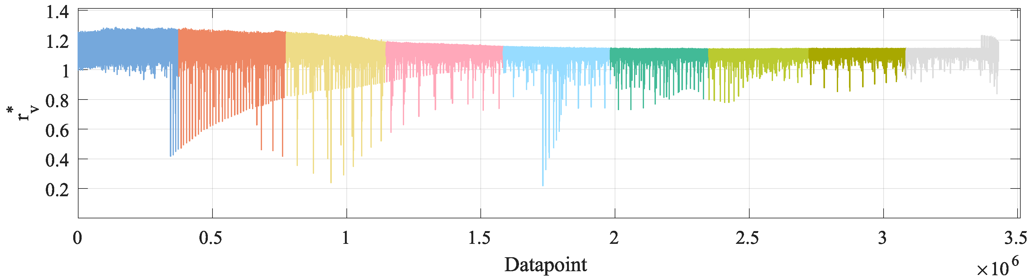
Figure 4.
Histogram of the generated dataset. Each color indicates a velocity range of the reference data.
Figure 4.
Histogram of the generated dataset. Each color indicates a velocity range of the reference data.
Figure 5.
Methodology for the data processing.
Figure 5.
Methodology for the data processing.
Figure 6.
Overview of the data selection process.
Figure 6.
Overview of the data selection process.
Figure 7.
Graphical depiction of the sample generation for .
Figure 7.
Graphical depiction of the sample generation for .
Figure 8.
Overview of the data balancing process.
Figure 8.
Overview of the data balancing process.
Figure 9.
Overview of the data splitting process.
Figure 9.
Overview of the data splitting process.
Figure 10.
The order of the first 100 training samples. Each color indicates the target velocity range as shown in
Figure 4.
Figure 10.
The order of the first 100 training samples. Each color indicates the target velocity range as shown in
Figure 4.
Figure 11.
Model architecture of the TNN based on [
17].
Figure 11.
Model architecture of the TNN based on [
17].
Figure 12.
Learning rate with respect of the training epoch for the hyper-parameter optimization. , , , , , , , , and .
Figure 12.
Learning rate with respect of the training epoch for the hyper-parameter optimization. , , , , , , , , and .
Figure 13.
Training loss with respect of the training epoch for the hyper-parameter optimization. , , , , , , , , and .
Figure 13.
Training loss with respect of the training epoch for the hyper-parameter optimization. , , , , , , , , and .
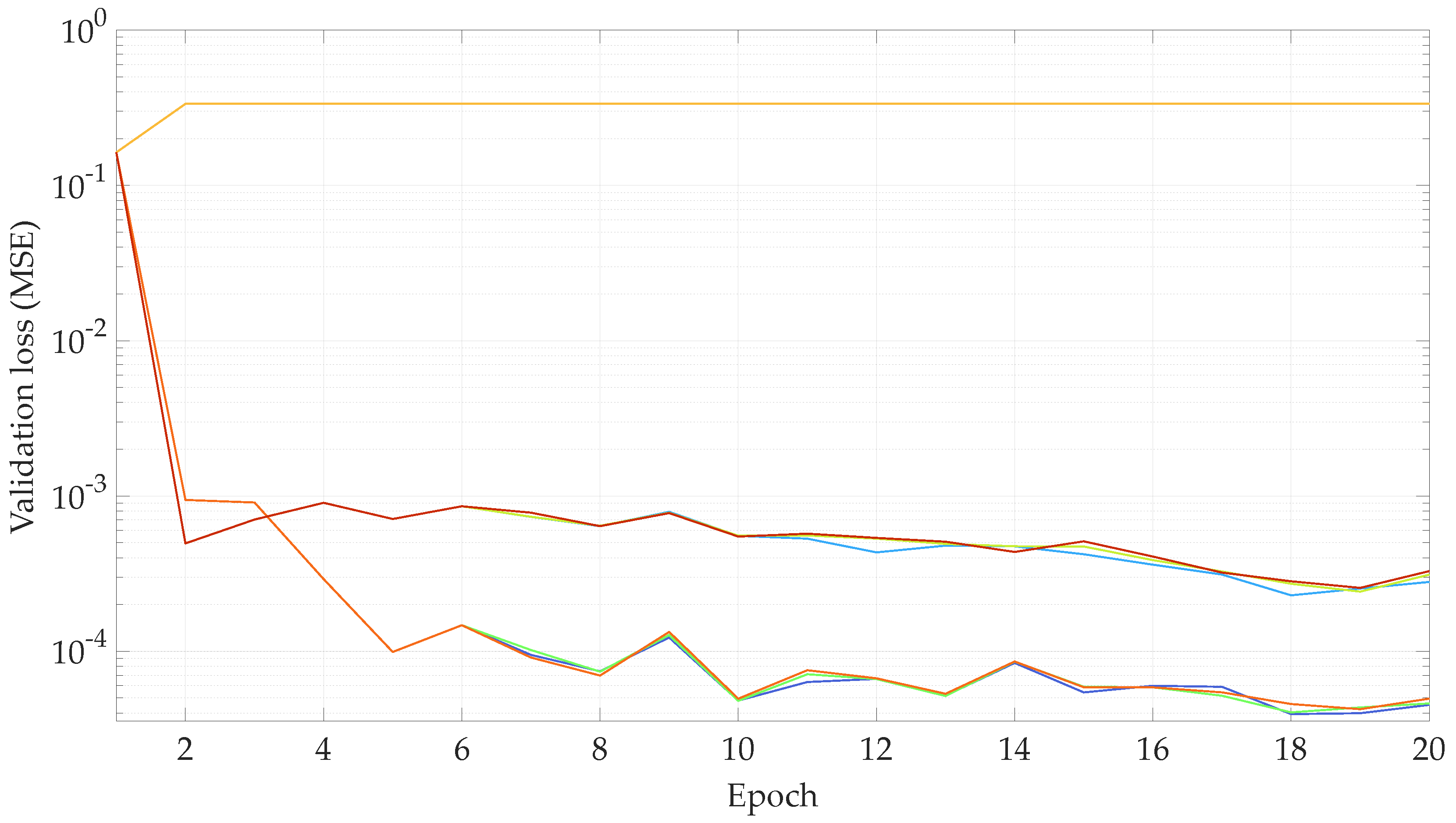
Figure 14.
Validationloss with respect of the validation epoch for the hyper-parameter optimization. , , , , , , , , and .
Figure 14.
Validationloss with respect of the validation epoch for the hyper-parameter optimization. , , , , , , , , and .
Figure 15.
Comparisonbetween the reference , expert and OBD velocities.
Figure 15.
Comparisonbetween the reference , expert and OBD velocities.
Figure 16.
Mathematical relation for the different velocity groups: –, –, –, –, –, –, –, –, –.
Figure 16.
Mathematical relation for the different velocity groups: –, –, –, –, –, –, –, –, –.
Figure 17.
Mathematical relation for the different velocity groups: –, –, –, –, –, –, –, –, –.
Figure 17.
Mathematical relation for the different velocity groups: –, –, –, –, –, –, –, –, –.
Table 1.
Selected parameters of the model based on TNN.
Table 1.
Selected parameters of the model based on TNN.
| Parameter | Value |
|---|
| # Encoder layers | 6 |
| # Encoder sub-layers | 2 |
| # Decoder layers | 6 |
| # Decoder sub-layers | 3 |
| # Attention heads | 8 |
| # Hidden dimension Feed Forward Network | 2048 |
| # Model dimension | 512 |
| # Attention queries dimension | 64 |
| # Attention keys dimension | 64 |
| # Attention values dimension | 64 |
Table 2.
Evaluation metrics for the baseline model for each of the velocity ranges.
Table 2.
Evaluation metrics for the baseline model for each of the velocity ranges.
| Group | MAE
| RMSE
| | MPE
| MAPE
|
|---|
| – | 0.129 | 0.191 | 0.984 | −0.173 | 0.020 |
| – | 0.122 | 0.221 | 0.973 | −0.004 | 0.010 |
| – | 0.145 | 0.217 | 0.977 | −0.001 | 0.080 |
| – | 0.192 | 0.252 | 0.967 | 0.003 | 0.008 |
| – | 0.180 | 0.237 | 0.974 | 0.005 | 0.007 |
| – | 0.181 | 0.251 | 0.970 | 0.004 | 0.006 |
| – | 0.176 | 0.247 | 0.971 | 0.003 | 0.005 |
| – | 0.197 | 0.269 | 0.964 | 0.003 | 0.005 |
| – | 0.181 | 0.262 | 0.941 | 0.003 | 0.004 |
| – | 0.167 | 0.240 | 0.999 | 0.001 | 0.008 |
Table 3.
Evaluation metrics for the TNN model when trained with input sequences of different lengths.
Table 3.
Evaluation metrics for the TNN model when trained with input sequences of different lengths.
| Input Length | MAE | RMSE | | MPE | MAPE | Time |
|---|
| | | | | | |
| 1 | 0.278 | 0.361 | 0.999 | −0.001 | 0.015 | 0.0325 ± 0.0037 |
| 2 | 0.472 | 0.604 | 0.998 | 0.015 | 0.023 | 0.0341 ± 0.0036 |
| 3 | 0.438 | 0.545 | 0.998 | 0.017 | 0.023 | 0.0340 ± 0.0036 |
| 4 | 0.333 | 0.419 | 0.999 | 0.002 | 0.019 | 0.0345 ± 0.0035 |
| 5 | 0.327 | 0.435 | 0.999 | −0.012 | 0.017 | 0.0349 ± 0.0038 |
| 10 | 0.360 | 0.453 | 0.999 | −0.008 | 0.018 | 0.0356 ± 0.0030 |
| 15 | 0.362 | 0.458 | 0.999 | 0.010 | 0.017 | 0.0356 ± 0.0027 |
| 20 | 0.374 | 0.481 | 0.999 | −0.007 | 0.016 | 0.0377 ± 0.0032 |
Table 4.
Evaluation metrics for the TNN model when trained with different database sizes.
Table 4.
Evaluation metrics for the TNN model when trained with different database sizes.
| Database Size | MAE
| RMSE
| | MPE
| MAPE
|
|---|
| 1000 | 0.863 | 1.037 | 0.999 | −0.017 | 0.057 |
| 5000 | 0.482 | 0.570 | 0.998 | −0.002 | 0.028 |
| 10,000 | 0.252 | 0.310 | 0.998 | −0.007 | 0.011 |
| 50,000 | 0.251 | 0.312 | 0.999 | 0.005 | 0.013 |
| 100,000 | 0.223 | 0.320 | 0.999 | −0.002 | 0.010 |
| 500,000 | 0.210 | 0.273 | 0.999 | −0.002 | 0.010 |
| 603,828 | 0.167 | 0.240 | 0.999 | −0.001 | 0.008 |
Table 5.
MAE for the OBD vs. reference sensor comparison and the MAE for the inference of the TNN vs. reference sensor comparison. Database size: 603,828.
Table 5.
MAE for the OBD vs. reference sensor comparison and the MAE for the inference of the TNN vs. reference sensor comparison. Database size: 603,828.
| Group | MAE-TNN
| MAE()
| Error Variation
% |
|---|
| – | 0.129 | 0.753 | −82.87 |
| – | 0.122 | 1.462 | −91.48 |
| – | 0.145 | 2.135 | −93.21 |
| – | 0.192 | 2.812 | −93.17 |
| – | 0.180 | 3.385 | −94.68 |
| – | 0.181 | 4.052 | −95.53 |
| – | 0.176 | 4.735 | −96.28 |
| – | 0.197 | 5.434 | −96.37 |
| – | 0.181 | 6.248 | −97.10 |
| – | 0.167 | 3.480 | −95.07 |
Table 6.
MAE for the OBD vs. reference sensor comparison and the MAE for the inference of the TNN vs. reference sensor comparison. Database size: 1000.
Table 6.
MAE for the OBD vs. reference sensor comparison and the MAE for the inference of the TNN vs. reference sensor comparison. Database size: 1000.
| Group | MAE-TNN
| MAE()
| Error Variation
% |
|---|
| – | 1.864 | 0.753 | +147.54 |
| – | 0.360 | 1.462 | −74.86 |
| – | 0.630 | 2.135 | −70.49 |
| – | 0.744 | 2.812 | −73.54 |
| – | 0.992 | 3.385 | −70.69 |
| – | 1.040 | 4.052 | −74.33 |
| – | 0.588 | 4.735 | −87.58 |
| – | 0.946 | 5.434 | −82.59 |
| – | 0.603 | 6.248 | −90.35 |
| – | 0.863 | 3.480 | −74.51 |
Table 7.
Synchronization errors between an OBD and a reference sensor measurement. # of measurements: 3,428,099.
Table 7.
Synchronization errors between an OBD and a reference sensor measurement. # of measurements: 3,428,099.
| Group | | mean | | |
|---|
| | | | |
| – | 0.0 | 0.0025 | 0.0098 | 0.346 |
| – | 0.0 | 0.0024 | 0.0099 | 0.349 |
| – | 0.0 | 0.0025 | 0.0099 | 0.349 |
| – | 0.0 | 0.0025 | 0.0099 | 0.349 |
| – | 0.0 | 0.0025 | 0.0097 | 0.342 |
| – | 0.0 | 0.0025 | 0.0098 | 0.346 |
| – | 0.0 | 0.0025 | 0.0099 | 0.349 |
| – | 0.0 | 0.0025 | 0.0092 | 0.325 |
| – | 0.0 | 0.0025 | 0.0099 | 0.349 |
| – | 0.0 | 0.0025 | 0.0099 | 0.349 |
Table 8.
MAE for vs. and the MAE for the inference of the TNN vs. . Database size: 603,828.
Table 8.
MAE for vs. and the MAE for the inference of the TNN vs. . Database size: 603,828.
| Group | MAE-TNN
| MAE ()
| Error Variation
% |
|---|
| – | 0.129 | 1.539 | −91.62 |
| – | 0.122 | 1.108 | −88.99 |
| – | 0.145 | 0.706 | −79.46 |
| – | 0.192 | 0.365 | −47.40 |
| – | 0.180 | 0.180 | 0.00 |
| – | 0.181 | 0.436 | −58.49 |
| – | 0.176 | 0.823 | −78.61 |
| – | 0.197 | 1.256 | −84.62 |
| – | 0.181 | 1.809 | −89.99 |
| – | 0.167 | 0.927 | −81.98 |
Table 9.
MAE for vs. and the MAE for the inference of the TNN vs. . Database size: 1000.
Table 9.
MAE for vs. and the MAE for the inference of the TNN vs. . Database size: 1000.
| Group | MAE-TNN
| MAE ()
| Error Variation
% |
|---|
| – | 1.864 | 1.539 | 21.12 |
| – | 0.360 | 1.108 | −67.51 |
| – | 0.630 | 0.706 | −10.76 |
| – | 0.744 | 0.365 | 103.84 |
| – | 0.992 | 0.180 | 451.11 |
| – | 1.040 | 0.436 | 138.53 |
| – | 0.588 | 0.823 | −28.55 |
| – | 0.946 | 1.256 | −24.68 |
| – | 0.603 | 1.809 | −66.67 |
| – | 0.863 | 0.927 | −6.90 |
Table 10.
Relation
according to Equation (
26). # of measurements: 3,428,099.
Table 10.
Relation
according to Equation (
26). # of measurements: 3,428,099.
Group
| | mean | |
|
|---|
| – | 0.001 | 0.486 | 0.790 | 0.789 |
| – | 0.070 | 0.718 | 0.898 | 0.828 |
| – | 0.001 | 0.809 | 0.912 | 0.911 |
| – | 0.347 | 0.861 | 0.911 | 0.564 |
| – | 0.062 | 0.889 | 0.921 | 0.858 |
| – | 0.546 | 0.910 | 0.934 | 0.388 |
| – | 0.608 | 0.927 | 0.949 | 0.341 |
| – | 0.689 | 0.939 | 0.959 | 0.271 |
| – | 0.689 | 0.952 | 1.043 | 0.353 |
| – | 0.001 | 0.833 | 1.043 | 1.042 |
Table 11.
Relation
according to Equation (
27). # of measurements: 3,428,099.
Table 11.
Relation
according to Equation (
27). # of measurements: 3,428,099.
Group
| | mean | |
|
|---|
| – | 0.0 | 1.1001 | 1.2855 | 1.2855 |
| – | 0.0 | 1.1173 | 1.2805 | 1.2805 |
| – | 0.0124 | 1.1240 | 1.2518 | 1.2394 |
| – | 0.0168 | 1.1242 | 1.1911 | 1.1743 |
| – | 0.0280 | 1.1233 | 1.1572 | 1.1291 |
| – | 0.7319 | 1.1249 | 1.1469 | 0.4149 |
| – | 0.7800 | 1.1260 | 1.1454 | 0.3654 |
| – | 0.8544 | 1.1282 | 1.1464 | 0.2920 |
| – | 0.8390 | 1.1329 | 1.2304 | 0.3914 |
| – | 0.0 | 1.1222 | 1.2855 | 1.2855 |


 ,
, 


