1. Introduction
The worldwide COVID-19 pandemic has brought about many changes in our daily lives and struck a devastating blow to the global economy. It is widely recognized that airborne transmission serves as the primary pathway for the spread of COVID-19 via expiratory droplets, especially in indoor environments [
1]. During the viral outbreak, many people were infected due to exposure to virus droplets generated by human exhalation activities [
2,
3,
4]. Some infected patients spread the virus unknowingly without properly being examined because there is an incubation period that varies for different mutations and asymptomatic patients who never experience apparent symptoms [
5]. Reliable and efficient tracing and quarantining have become more important than ever to alert individuals to take actions to interrupt the transmission between people and further curb the spread of the disease. Contact tracing involves identifying, assessing, and managing people who are at risk of the infection, and tracking subsequent victims as recorded by the public health department [
6]; contact tracing can be performed via manual or digital methods. Since the manual contact tracing is labor-intensive and time-consuming and may be incomplete and inaccurate due to forgetfulness; automatic digital contact tracing has been widely researched in recent years [
7]. Usually, digital contact tracing applications are installed on portal devices, typically smartphones, to conveniently and intelligently realize tracing with the help of existing sensors based on various technologies, such as a global navigation satellite system (GNSS), Bluetooth, and Wi-Fi.
Contact tracing in indoor environments can complement the ones used in outdoor environments to enable comprehensive digital contact tracing. However, indoor contact tracing imposes unique technical challenges due to virus concentrations and unreliable GNSS signals in indoor environments [
8]. The virus concentration, which plays a critical role in calculating the amount of a virus we are exposed to and further assesses the infection risk, should be explicitly considered in indoor contact tracing applications [
3,
9]. The quantitative infection risk for a susceptible person is significantly associated with the quantity of the pathogen inhaled in the surrounding ambient air, from the respiratory droplets exhaled by infected individuals [
10]. Thus, inhaling a large amount of the virus in a short period, i.e., under the 15 min time mark, can greatly increase the infection risk, especially for so-called “superspreading events”, which invariably occur indoors [
11]. Moreover, the majority of time has to be spent by people in indoor contexts with plenty of daily activities performed. However, GNSS-based approaches do not work well in indoor environments due to signal attenuation. Phone-to-phone pairing-based methods using Bluetooth low energy (BLE) work only for direct face-to-face contact tracing scenarios and are inapplicable to indirect virus exposure in ambient aerosols. The expelled pathogen-containing particles can remain active in the air for hours without sufficient sanitization, especially in indoor environments, constructing a significant fraction of the virus concentration [
3]. Recently, vContact was proposed as a means to detect exposure to the virus with the consideration of asynchronous contacts by leveraging Wi-Fi networks, while the spatiotemporal dynamism in the virus concentration is not fully being considered [
8].
Although the virus concentration will gradually decrease due to inactivation, deposition, and air purification after the virus-laden droplets are exhaled, the poor air exchange rate, superspreaders, and more virulent variants will keep it at a relatively high concentration for a long time in an indoor environment [
9,
12]. The viral particles are continuously ejected by infected people at different locations, relying on human movement. Moreover, due to the initial motion state and environmental airflow, these droplets maintain a ceaseless transmission before they are removed and meet somewhere (at some time), which leads to constant changes in the virus concentration within the control volume [
13]. To accurately estimate the concentration, investigating the airborne transmission of these ejected particles is, thus, of fundamental importance in a closed environment because of the assemblage, in which human movement is implicitly involved to achieve the initial motion state of droplets [
13]. The qualitatively location-specific assessment of the viral concentration is proposed with the dual use of computational fluid dynamic simulations and surrogate aerosol measurements for different real-world settings [
14]. Moreover, the transmission of the virus brings about changes in the viral concentration of a specific location in an overall space, as well as the movements of people. Z. Li et al. analyzed the dispersion of cough-generated droplets in the wake of a walking person [
4].
To be precisely aware of the amount of the virus one is exposed to and to detect both direct and indirect contacts, an indoor spatiotemporal contact awareness (iSTCA) framework is proposed. Since the virus concentration (at different times in the same area) is not the same because of the dispersion and diffusion of the virus and human movements, we employed a self-contained PDR technique to calculate the human trajectory with accuracy and further achieve the location and time of the expelled virus droplets for the quantitative measurement of the concentration at any time in different spots. Moreover, based on the acquired changing virus concentration and reliable trajectories, the exposure time and distance of both direct and indirect contacts can be derived via cross-examination to realize quantitative spatiotemporal contact awareness.
Our main contributions are as follows:
To accurately present the virus concentrations at different times, we established quantitative virus concentration changes in various areas of indoor environments at different times by infected individuals. The viral-laden droplets were continuously released during the expiratory activities, moving forward. During the movements of viral-loaded droplets exhaled by infectious individuals at different locations and times, the virus instances met in certain spots at certain times and contributed to the calculation of the concentration. Finally, the concentration of each virus instance was integrated.
We properly selected PDR for the acquisition of the trajectory to conduct contact awareness without requiring extra infrastructure or being affected by coverage limitations compared with other indoor positioning techniques.
We considered various landmarks to calibrate the accumulative error for trajectory achievement by using PDR. A custom deep neural network using bidirectional long short-term memory (Bi-LSTM) and multi-head convolutional neural networks (CNNs) with residual concatenations were designed and implemented to extract temporal information in forward and backward directions and spatial features at various resolutions from built-in sensor readings for landmark identification.
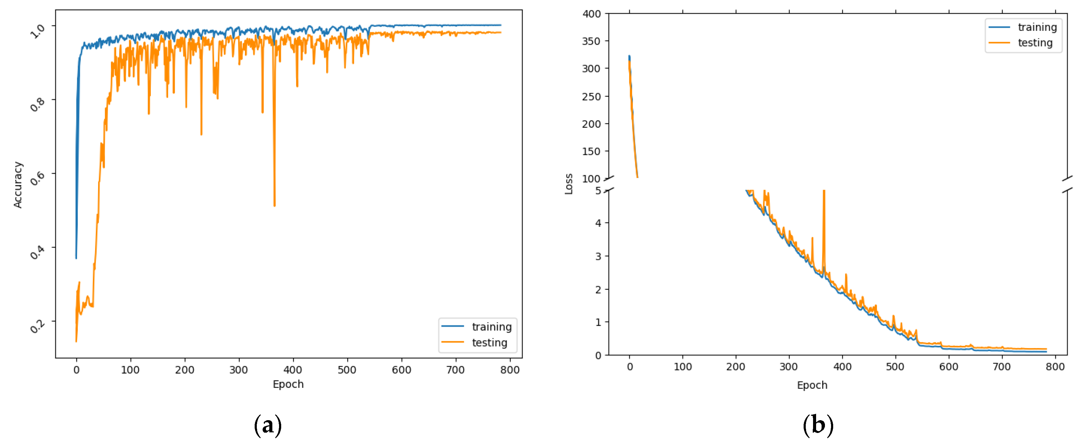
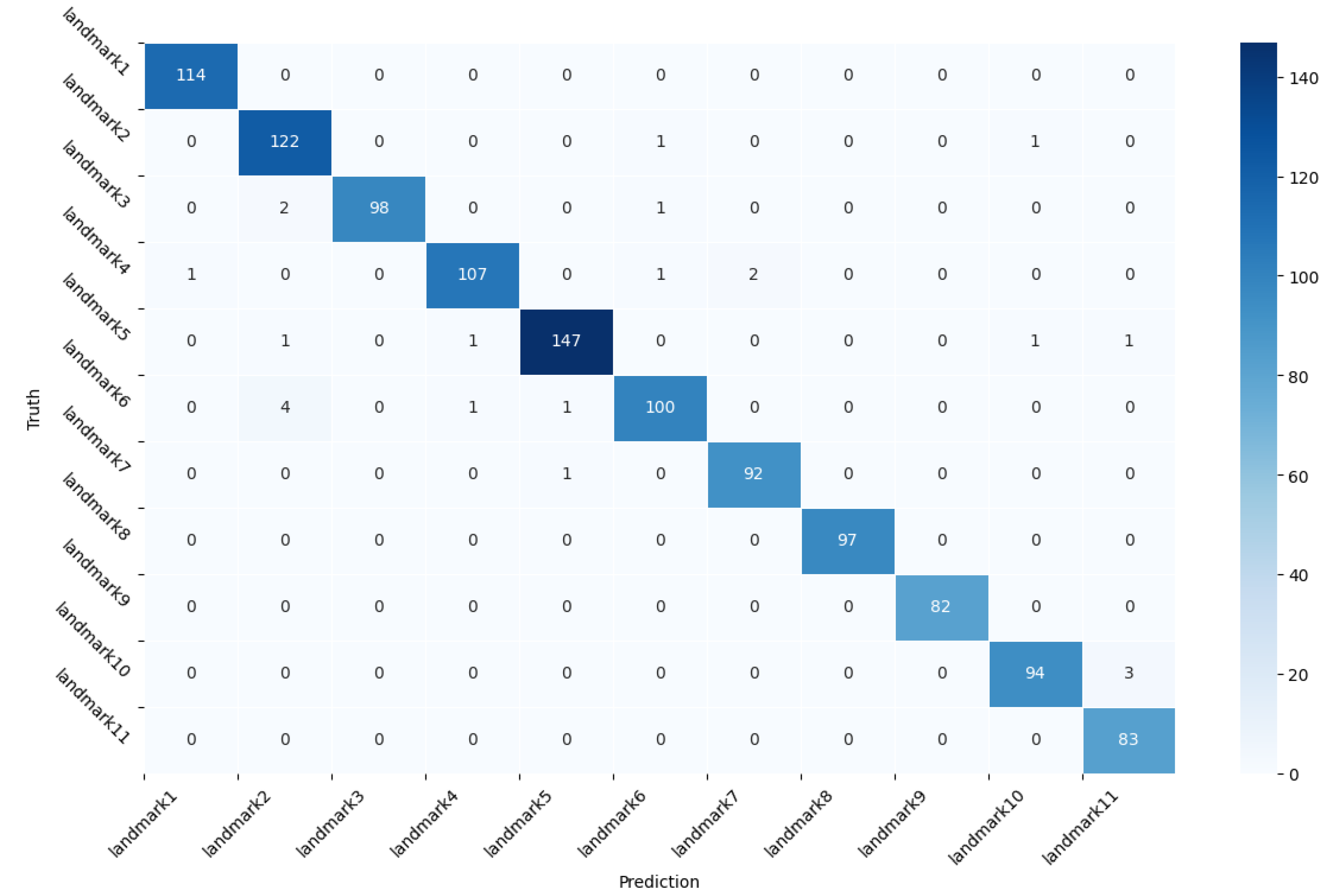
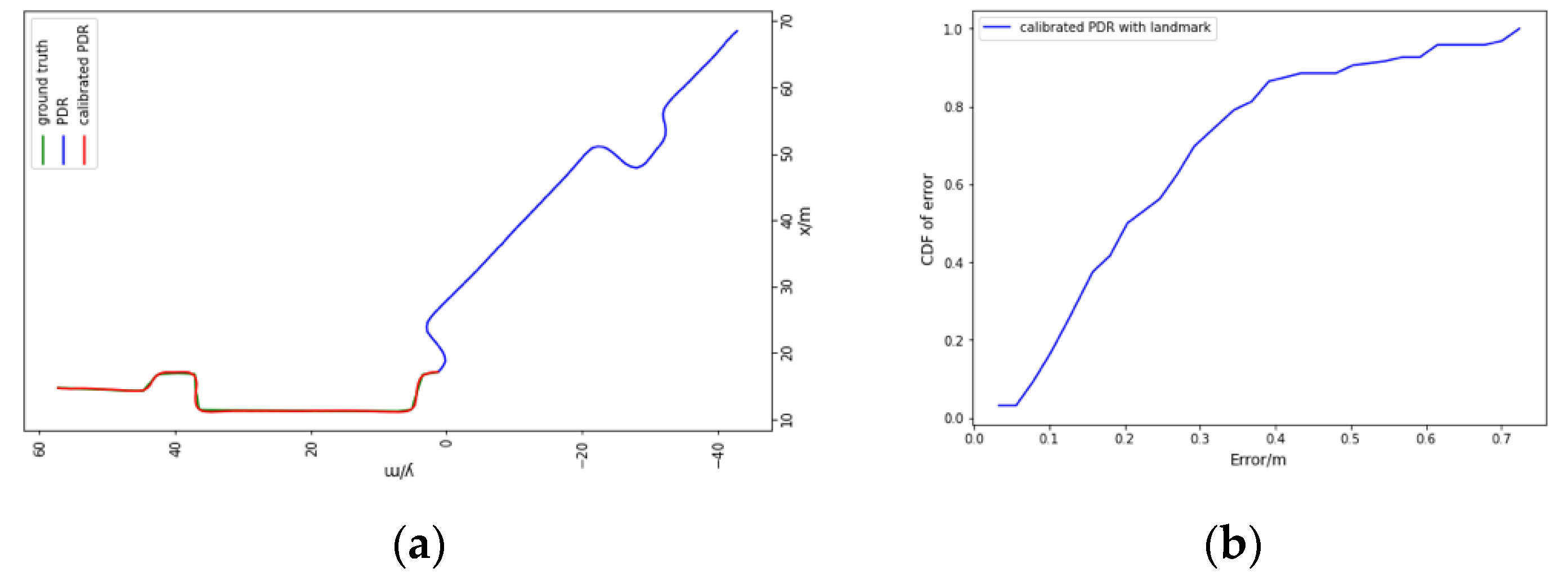
Additionally, we demonstrate the effectiveness of the proposed Bi-LSTM-CNN classification model for landmark identification through empirical experiments, as well as the performance of our proposed iSTCA system for quantitative spatiotemporal contact analytics.
The remainder of this paper is organized as follows. The related work about contact awareness and indoor localization techniques, including PDR, is reviewed in
Section 2. Definitions and preliminaries about virus concentrations and different contact types are introduced in
Section 3.
Section 4 introduces the theoretical methodology and the architecture of the proposed iSTCA. The experimental methodology and results based on the collected datasets are presented in
Section 5.
Section 6 reveals the limitations of this work. Finally, we present the conclusion and future work in
Section 7.
2. Related Work
Contact tracing is used to identify and track people who may have been exposed to a virus due to the prevalence of many infectious diseases in our society. To conduct contact tracing, it is necessary for the infected individuals to provide their visited locations and people whom they encountered based on the specific definitions of meetups for different diseases. Instead of interviews and questionnaires via traditional manual tracing, technology-aided contact tracing can track people at risk conveniently and intelligently. To reduce the spread of COVID-19 effectively, digital contact tracing, which generally depends on applications installed on smartphones, has been developed in both academia and industry, using various technologies, such as GNSS, Bluetooth, and Wi-Fi.
There are typically two approaches for encounter determinations, peer-to-peer proximity detection-based and geolocation-based. Peer-to-peer proximity can be estimated by the received signal strength (RSS) of wireless signals, such as Bluetooth and ultra-wideband (UWB), and the distance between two devices in geolocation-based approaches can be precisely derived from the cross-examination after obtaining the accurate location and trajectory with the help of localization techniques using various technologies, such as global positioning system (GPS), Wi-Fi, and PDR.
Some systems based on peer-to-peer proximity using Bluetooth or BLE have been implemented, and part of them are deployed by the governments of various countries, such as Australia (COVIDSafe), Singapore (Trace together), and the United Kingdom (NHS COVID-19 App) due to their ubiquitous embedding in mobile phones [
15]. Among these systems, the most representative protocols are Blue Trace and ROBERT [
11,
16]. The data from Bluetooth device-to-device communications are stored and checked against the data uploaded by the infector. In Blue Trace, the health authority contacts individuals who had a high probability of virus exposure, whereas ROBERT users need to periodically probe the server for their infection risk scores. In addition, Google and Apple provide a broadly used toolkit based on Bluetooth, named Google and Apple Exposure Notification (GAEN), to facilitate a contact tracing system in Android and iOS and curb the spread of COVID-19 [
17]. Despite some minor differences in implementation and efficiency, these schemes are all independently designed and very similar. When exposure is detected, the RSS in the communication data frame is utilized to estimate the distance between two devices and notify the user. However, it has been demonstrated that the signal strengths can only provide very rough estimations of the actual distances between devices, as they are affected by device orientation, shadowing, shading effects, and multipath losses in different environments [
18,
19]. Although it is difficult to measure the distances among users accurately by using Bluetooth and other technologies, the UWB radio technology has the capacity to measure distances at the accuracy level of a few centimeters, which is significantly bettering than Bluetooth [
20]. The use of UWB, however, has some significant drawbacks, including the fact that UWB is not widely supported by mobile devices, requires extra infrastructure, and is not energy efficient, which makes UWB less useful in practice [
21]. All of the above works that are based on calculated proximity using RSS do not consider the user’s specific physical location, resulting in unsatisfactory tracing results. Moreover, these approaches cannot be applied to the detection of temporal contact due to the dispersion and lifespan of the virus.
To achieve accurate geolocation in contact tracing, plenty of localization systems have been researched with the joint efforts of researchers and engineers in the past based on GNSS, cellular technology, radio frequency identification (RFID), and quick response (QR) code [
7]. GNSS can be used for contact tracing as the exact position of a person can be located and it is available globally. Many countries, including Israel (HaMagen 2.0) and Cyprus (CovTracer), use GPS-based contact tracing approaches [
15] as well. GNSS signals are usually weak in indoor environments due to the absence of the line of sight and the attenuation of satellite signals, as well as the noisiness of the environment. Many people may spend most of their time in indoor environments, which can result in limited contact coverage. It is difficult to detect contact based on cellular data due to the large coverage of cell towers and high location errors [
8]. RFID was used to reveal the spread of infectious diseases and detect face-to-face contact in [
22,
23]. QR codes for contact tracing require users to check in at various venues by scanning the placed QR codes manually to record their locations and times, which are deployed in some countries, such as New Zealand (NZ COVID Tracer) [
15]. However, special devices or codes have to be deployed at scale for data collection. Recently, some protocols were proposed for Wi-Fi-based contact tracing with the pre-installed Wi-Fi Access Point. WiFiTrace was proposed by proposed in [
24]. WiFiTrace is a network-centric contact tracing approach with passive Wi-Fi sensing and without client-side involvement, in which the locations visited are reconstructed by network logs; graph-based model and graph algorithms are employed to efficiently perform contact tracing. Wi-Fi association logs were also investigated in [
25] to infer the social intersections with coarse collocation behaviors. Li et al. utilized active Wi-Fi sensing for data collection; they leveraged signal processing approaches and similarity metrics to align and detect virus exposure with temporally indirect contact [
8]. As the changes in virus concentrations over time (due to the transmission of aerosols and environmental factors) are not considered, their results are in relatively low spatiotemporal resolutions. The approach presented in [
26] divides contact tracing into two separate parts, duration and distance of exposure. The duration is captured from the Wi-Fi network logs and the distance is calculated by the PDR positioning trajectory, calibrated by recognized landmarks with the help of a CNN, ensuring the performance of contact tracing. Although integration with the existing infrastructure is beneficial in mitigating the deployment costs, it may not fully satisfy the requirements of contact tracing with the high spatiotemporal resolution because of the absent coverage [
27]. The trajectory obtained by the PDR technique, without requiring special infrastructure, can improve the coarse-grained duration and make it fine-grained. This can enable the development of a contact-tracing environment that considers the virus lifespan in detail.
One of the ultimate goals of contact awareness systems is to estimate the risk based on the recorded encounter data [
28]. Moreover, with the exposure duration and distance obtained, the virus concentration is significant to determine the exposed viral load, which is closely associated with the infection risk [
29]. Typically, the virus concentration in a given space depends on the total amount of viral load contained in the viable virus-laden droplets in the air and maintains a downward trend because of the self-inactivation and environmental factors. Researchers presented the qualitative location-specific assessment of viral concentration with the dual use of computational fluid dynamic simulations and surrogate aerosol measurements for different real-world settings [
14]. The practical viral loads emitted by contagious subjects based on the viral loads in the mouth (or sputum) with various types of respiratory activities and activity levels are presented in [
29]. Furthermore, to quantitatively shape the virus concentration in a targeted environment at different times, the constant viral load emission rate is adopted with the virus removal rate, including the air exchange rate, particle sediment, and viral inactivation rate in [
30].
The aforementioned contact tracing research usually only considers the static virus concentration without considering the exposure to the environmental virus and dynamism in the virus concentration. Moreover, in contrast to the qualitative estimation of exposure risks that can be achieved in previous works, there is a lack of sufficient quantitative awareness about the concentrations of contracted viruses. Such awareness would be useful in our daily lives to protect ourselves from virus infections.
4. Methodology
This work utilizes the trajectories, including the spatial position coordinates and time obtained by the PDR technique to quantitatively estimate the time-dependent changes in the virus quanta concentration derived from the movement and lifespan of the virus in various places of the considered indoor environment. The overview of the proposed scheme is systematically introduced in
Section 4.1. In
Section 4.2, we provided the data processing approaches utilized in PDR-based trajectory construction and the estimation of droplet exhalation. The PDR technique (with a calibration of the landmark recognized by a landmark identification model based on a residual Bi-LSTM and CNN structure) is discussed in
Section 4.3. Further, the contact awareness model relying on the precisely constructed pedestrian trajectory is detailed in
Section 4.4.
4.1. System Overview
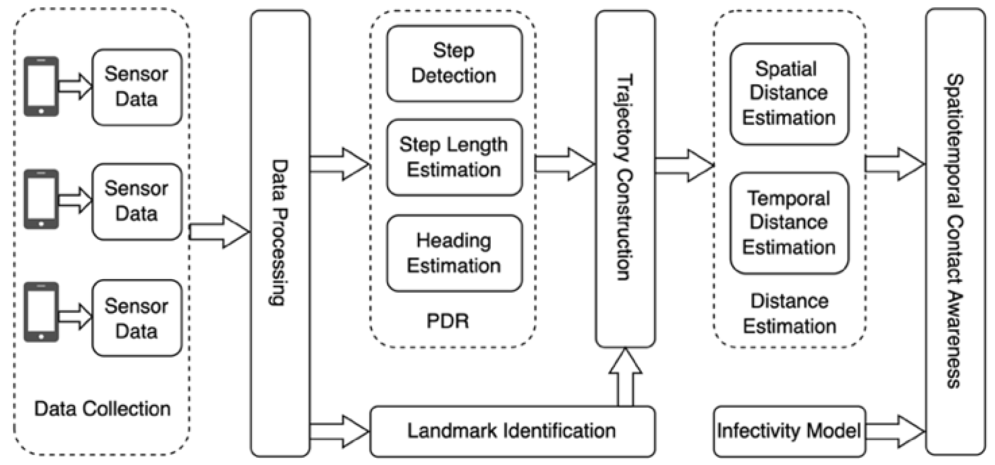
An overview of the proposed iSTCA system is presented in
Figure 1. More precisely, the data flow of various sensors for the analysis was primarily collected from the existing sensors in handhold smartphones, which record the changes in the environment and body motion. The signals need to be processed, including data filtering and scaling, to reduce the noise for a better state of motion estimation before training the landmark identification model and performing the PDR. The trajectory can be achieved based on the PDR technique and properly corrected with the assistance of the identified landmark distinguished by the trained landmark recognition model. The trajectory is defined as a set of points consisting of the time and position,
where
represents the location coordinates and
is the moment when the individual passes the location. The virus quanta concentrations in different spaces at various moments can be measured quantitatively to achieve sufficient awareness with the help of the estimated spatial distance, temporal distance, and infectivity model, as shown in Equation (1).
4.2. Data Preprocessing
Data alignment. The same sampling rate for data collection is set to 50 Hz due to the low frequency of human movements [
32]. Although the constant rate is defined, the time interval between the recorded adjacent readings of each sensor is not always the same because of the observational error and random error, and it oscillates within a certain range in practice. To acquire the same number of samples for conveniently performing the subsequent procedures, we take the timestamp of the first data collected as the starting time to align the sensor readings at the same time interval with the help of data interpolation.
Data interpolation. During the practical data collection using smartphone sensors, some data points in the acquired dataset are lost due to malfunctioning; such data points are typically replaced by 0, NaN, or none [
33]. To fill in the missing values, the data interpolation technique was developed, in which the new data point is estimated based on the known information. Linear interpolation, as the prevalent type of interpolation approach, was adopted in this paper, using linear polynomials to construct new data points [
34]. Generally, the strategy for linear interpolation is to use a straight line to connect the known data points on either side of the unknown point and, thus, it is defined as the concatenation of linear interpolation between each pair of data points on a set of samples.
Data filtering. Due to the environmental noise and interference caused by the unconscious jittering of the human body, there are many undesirable components in the obtained signals that need to be dealt with [
34]. This usually means removing some frequencies to suppress interfering signals and reduce the background noise. A low-pass filter is a type of electronic filter that attempts to pass low-frequency signals through the filter unchanged while reducing the amplitude of signals with a frequency above what is known as the cutoff frequency. A Butterworth low-pass filter with a cutoff frequency of 3 Hz is applied to denoise and smooth the raw signals.
Data scaling. The difference in the scale of each input variable increases the difficulty of the problem being modeled. If one of the features has a broad range of values, the objective functions of THE established model will be highly probably governed by the particular feature without normalization, suffering from poor performance during learning and sensitivity to input values and further resulting in a higher generalization error [
35]. Therefore, the range of all data should be normalized so that each feature contributes approximately proportionately to the final result. Standardization makes the values of each feature in the data have zero means by subtracting from the mean in the numerator and unit variance, as shown in Equation (3):
where the
is the standardized data,
represents the number of data channels, and
and
are the mean and standard deviations of the
-th channel of the samples [
35]. This method is widely used for normalization in many machine learning algorithms and is also adopted in this work to normalize the range of data we obtained.
Data segmentation. A sensor-based landmark recognition model is typically fed with a short sequence of continuously recorded sensor readings since only a single data point cannot reflect the characteristics of landmarks. The sequence consists of all the channels of selected sensors. To preserve the temporal relationship between the acquired data points with the aligned times, we partition the multivariate time-series sensor signals into sequences or segments leveraging the sliding operation, which consists of 128 samples (corresponding to 2.56 s for the sampling frequency at 50 Hz) [
34,
36]. It is noteworthy that the length of the window is picked empirically to achieve the segments for all considered landmarks, in which the features of the landmarks can be precisely captured to promote the landmark identification model training [
32,
37].
4.3. PDR-Based Trajectory Construction Model
For the quantitative evaluation of the virus quanta concentration, the precise spatial distance and temporal distance between two individuals should be efficiently estimated. To reach this objective, a variety of indoor positioning techniques have been proposed for various scenarios. The widely studied fingerprinting-based method relies on the latest fingerprint database that needs to be precisely updated in time. In addition to the time-consuming and labor-intensive collection and re-establishment, the instability of RSS due to environmental uncertainties poses another challenge to the accuracy [
38]. Moreover, coverage and distribution are also not satisfied in countries with poor ICT infrastructure [
39]. Therefore, the self-contained PDR algorithm without extra requirements and coverage limitations is employed in this work, and its accuracy is improved by the identified landmark.
4.3.1. PDR
Since PDR does not need additional equipment or a pre-survey, it has a wide range of potential applications for the indoor positioning of pedestrians. It relies on the inertial sensors extensively existing in mobile devices, e.g., smartphones, to acquire information about the user’s movements, which are then combined with the user’s previous location to estimate the present position and further achieve complete trajectory. The equation utilized for location estimation is as follows:
where
is the pedestrian position at time
,
is the step length, and
details the heading direction of the pedestrian [
40].
As mobile technology continues to evolve, a growing number of physical sensors are being installed in smartphones and, thus, various combinations of sensors can provide increasingly rich information, which makes PDR more feasible and accessible. A typical PDR consists of three main components: step detection, step-length estimation, and heading estimation [
41].
Step detection. As the most popular method for accurate step detection, peak detection is employed in this paper, which relies on the repeating fluctuation patterns during human movement. Using the smartphone’s accelerometer to determine whether the pedestrian is stationary, or walking is straightforward as it directly reflects the moving acceleration. The magnitude of acceleration on three dimensions
instead of the vertical part is employed as the input for peak findings to improve the accuracy, which can be expressed as:
where
denote the three-axis accelerometer values in the smartphone [
42]. A peak is detected when
is greater than the given threshold. To further enhance the performance, the low-pass filter is further applied to the magnitude to reduce the signal noise. Due to the acceleration jitter, the incumbently detected peak points need to be eliminated. Hence, an adaptive threshold technique of the maximum and minimum acceleration is adopted to fit different motion states with a time interval limitation between adjacent detected steps.
Stride length estimation. Various linear and nonlinear methods are proposed to estimate the step length, which varies from person to person because of different walking postures determined by various factors, including height, weight, and step frequency. Therefore, it is not easy to precisely construct the same step-length estimation model. Some researchers assume that the step length is a static value affected by the individual characteristics of different users. On the contrary, the empirical Weinberg model estimates the stride length according to the dynamic movement state, which is closer to reality [
43]. The model is given by:
where
is the dynamic value concerned with the acceleration of each step and
are the maximum and minimum accelerations for each step [
44].
Heading estimation. Heading information is a critical component for the entire PDR implementation, which seriously affects localization accuracy. To avoid the accumulative error in the direction estimation based on the gyroscope, and short-term direction disturbances based on the magnetometer, the combination of the gyroscope and magnetometer is typically adopted for heading estimation [
42]. The current magnetometer heading signals, current gyroscope readings, and previously fused headings are weight-averaged to form the fused heading. The weighting factor is adaptive and is based on the magnetometer’s stability as well as the correlation between the magnetometer and the gyroscope [
44]. As they are already fused in the rotation vector achieved from the rotation sensor in the smartphone, the heading change can be calculated by a rotation matrix transformed from the rotation vector [
45]. The rotation vector is defined as:
, and the matrix is defined as
. The heading direction on three dimensions can be evaluated by:
4.3.2. Landmark Identification Model
Although PDR methods can estimate the location and trajectory of pedestrians, low-cost inertial sensors built into smartphones provide poor-quality measurements, resulting in accuracy degradation. Moreover, the cumulative error, including the heading estimation caused by the gyroscope and step-length estimation error caused by an accelerometer, could be produced in the long-term positioning using PDR, increasing the challenge of precise localization collection. Therefore, it is necessary to prepare the reference points with the correct positions known during the movement to reduce the accumulated errors when the user passes. Spatial contexts, such as landmarks, can be properly chosen to calibrate the localization error based on the inherent spatial information without additional deployment costs. Landmark is defined as a spatial point with salient features and semantic characteristics from its near environment in indoor positioning systems, such as corners, stairs, and elevators [
27]. These features can be observed for identification in one or a combination of different sensors as people pass through the landmark. The locations of these landmarks are presented by geographical coordinates or the relationships with other locations/areas, where people perform specific and predictable activities. Changes in motion are reflected in sensor readings, and different motions present different patterns. The specific activities that people perform when passing landmarks are also reflected in at least one sensor. Using the data of one sensor or the combination of data from multiple sensors, the changing pattern of a specific activity can be identified, and then the landmark can be recognized [
46]. The identified landmark can be used as an anchor point to correct the path we obtained and improve the performance of the calculated trajectory.
Landmark identification involves classifying the sequences of various sensor data recorded at regular intervals by sensing devices, usually smartphones, into a well-defined landmark, which has been extensively regarded as a problem of multivariate time series classification. To address this issue, it is critical to extract and learn the features comprehensively to determine the relationship between sensing information and movement patterns. In recent years, numerous features have been attained in many studies on certain raw signal statistical aspects, such as variance, mean, entropy, kurtosis, correlation coefficients, or frequency domains via the integration of cross-formal codings, such as signals with Fourier transform and wavelet transform [
47]. Moreover, the special thresholds of different features for various kinds of landmark recognition are specifically analyzed. For instance, the threshold of angular velocity produced by a gyroscope is usually used to detect the corner landmark, the acceleration changes can recognize the stairs. The combinations of different thresholds of various sensors forming the decision tree can detect the standing motion state to further distinguish common landmarks, such as corners, stairs, and elevators [
48,
49]. However, despite high accuracy, the calculation, extraction, and selection of features of different sensors for various landmarks are heuristic (with professional knowledge and expertise of the specific domain), time-consuming, and laborious [
47].
To facilitate feature engineering and improve performance, artificial neural networks based on deep learning techniques have been employed to conduct activity identification without hand-crafted extraction. Deep learning techniques have been applied in many fields to solve practical problems with remarkable performance, such as image processing, speech recognition, and natural language processing, to solve practical problems [
50,
51]. Many kinds of deep neural networks have been introduced and investigated to handle landmark identification based on the complexity and unsureness of human movements. Additionally, CNN and LSTM are widely adopted with high accuracy rate activity recognition among the applied networks. CNN is commonly separated into numerous learning stages, each of which consists of a mix of convolutional operation and nonlinear processing units, as follows:
where
reveals the latent representation of the
-th feature map of the current layer,
is the activation function,
denotes the convolution operation,
indicates the
-th feature map of the group of the feature maps
achieved from the upper layer,
and
express the weights matrix and the bias of the
-th feature map of the current layer, receptively [
52]. In our model, the rectified linear units (ReLU) were employed as the activation functions to subsequently conduct the non-linear transformation to obtain the feature maps, denoted by:
More importantly, the convolution operation in CNN can efficiently capture the local spatial correlation features by limiting the hidden unit’s receptive field to be local [
53]. CNN considers each frame of sensor data as independent and extracts the features for these isolated portions of data without considering the temporal contexts beyond the boundaries of the frame. Due to the continuity of sensor data flow produced by the user’s behavior, local spatial correlations and temporally long-term connections are both important to identify the landmark [
52]. LSTMs with learnable gates, which modulate the flow of information and control when to forget previous hidden states, as variants of vanilla recurrent neural networks (RNNs), allow the neural network to effectively extract the long-range dependencies of time-series sensor data [
54]. The hidden state for the LSTM at time
is represented by:
where
and
are the hidden state at time
and
, respectively,
is the activation function,
and
are the weight matrices between the parts, and
symbolizes the hidden bias vector. The standard LSTM cells barely extract the features from the past movements, ignoring the future part. To comprehensively capture the information for landmark identification, the Bi-LSTM is applied to access the context in both the forward and backward directions [
55].
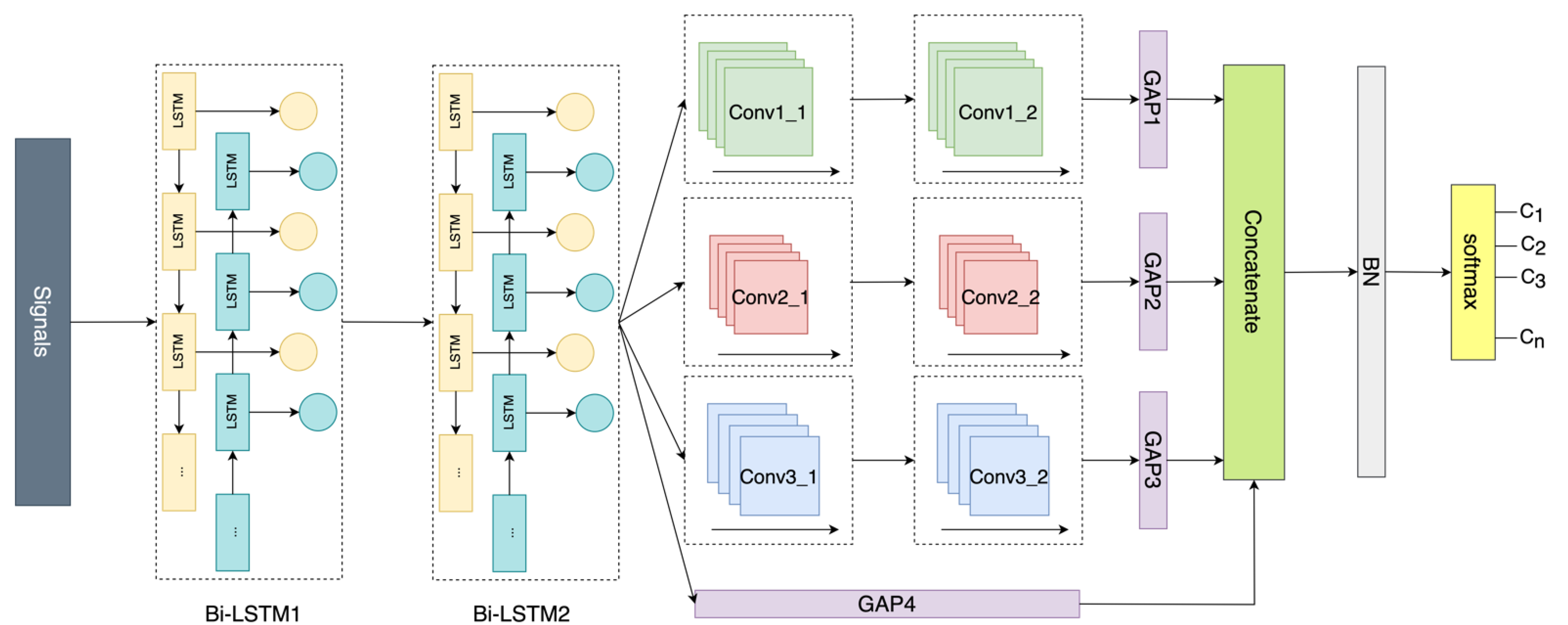
Therefore, both Bi-LSTM and CNN are involved in capturing the spatial and temporal features of signals for landmark identification. The architecture of the proposed landmark identification is shown in
Figure 2. It performs the function of landmark recognition using the residual concatenation for classification, followed by Bi-LSTM and multi-head CNN. When preprocessed data segmentations of multiple sensors come, the inherent temporal relationship is extracted sequentially by two Bi-LSTM blocks that consist of a Bi-LSTM layer, a batch normalization (BN) layer, an activation layer, and a dropout layer. BN is a method used to improve training speed and accuracy with the mitigation of the internal covariate shift through normalization of the layer inputs by recentering and re-scaling [
34]. Next, multi-head CNN blocks with varying kernels size are followed to learn the spatial features at various resolutions. Each convolutional block is made of four layers: a one-dimensional (1D) convolutional layer, a BN layer, an activation layer, and a dropout layer. To accommodate the three-dimensional input shape (samples, time steps, input channels) of the 1D convolutional layer, we retain the output of the hidden state in the Bi-LSTM layer. Then the acquired spatial and temporal features are combined, namely the concatenations of the outputs of the multi-head CNNs and Bi-LSTMs. To reduce the parameters and avoid overfitting, the global average pooling layer (GAP) with no parameter to optimize rather than the traditional fully connected layer is applied before combining the outputs [
32]. Finally, the concatenated features are transmitted into a BN layer to re-normalize before being fed into a dense layer with a softmax classifier to generate the probability distribution over classes.
4.4. Contact Awareness with Trajectory
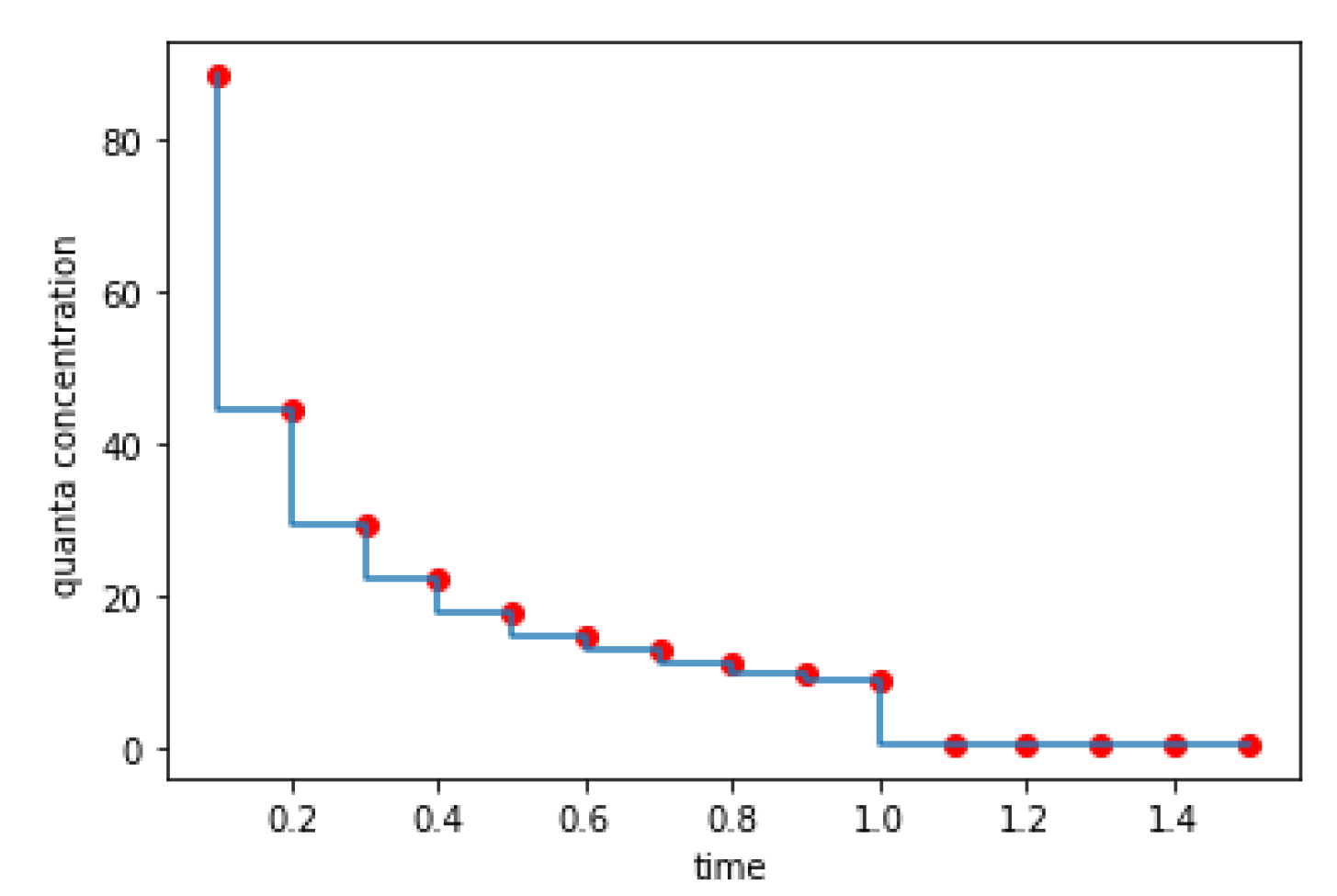
Exhalation and inhalation respiratory activities are constantly alternating (e.g., each breath consists of 2.5 s of continuous exhalation and 2.5 s of continuous inhalation), and droplets are continuously being released from the respiratory tract with a horizontal velocity during the process of exhalation with the same direction as the movement of the human. The particles exhaled at each moment will continue to move forward, starting from the user positions when they are expelled. The viral droplets exhaled from the infectious host are transported and dispersed into the ambient airflow before finally being inhaled by a susceptible person. Each exhalation lasts several seconds (e.g., 2.5 s), in which a long distance can be traveled for those who are in motion, and the initial position of droplets expelled cannot be accurately estimated in an indoor environment. Therefore, once complete, the exhalation period is divided into many short-term (e.g., 0.1 s) particle ejections. Because the interval is short, the continuous virus exhalation process can be converted into an instantaneous process, i.e., the virus is released instantly at the beginning of each interval. The virus-laden droplets expelled at different intervals maintain independent and identical motion patterns and the initial positions of the particles released in each interval can be regarded as the locations of the people at the initial moments. The virus-containing particles maintain a uniform motion of initially horizontal velocity (e.g., ) in the first second and then instantaneously will mix in the overall considered space. Meanwhile, the droplets are evenly distributed within the moved space. In the first movement phase of the exhaled droplets in each interval, the virus moves in the same direction as the people travel, which is called forward transmission. As for the backward transmission, in general, the initial velocity of the virus is faster than the speed of movement and the speed of airflow, so in the first phase, very few virus particles move in the opposite direction.
The movements of all viral-loaded droplets exhaled by infectious people at different locations will meet somewhere at some time and contribute to the calculation of concentration. To precisely present the virus quanta concentrations, the transmissions of all virus particles per exhalation sources from different origins and in different states are assumed to follow the same patterns, in which the particles keep constant initial velocity in the first second and then will instantly mix in the overall space. The time it takes for the virus to move to the current point and the contribution to the virus quanta in the present are estimated with the help of spatial distance and velocity. Thus, the quanta concentration in an indoor area at time
is measured by:
where
is the virus removal rate of the target space,
represents the virus generated in different places at different moments,
is the of the quanta emission rate of the infector at which the virus (
-th) is expelled,
is the time difference from the start of the experiment to present,
is the time difference between the current time and the originating time of the virus (
-th),
is the volume of the space that the
-th virus had passed since it was expelled to the present,
is the environmental virus quanta number,
is the virus exhaled by the infector that has evenly spread to the overall investigated space with the volume of
. Exhaled virus particles eventually become the environmentally well-mixed virus quanta, while different initial states induce different decays.
4.5. Spatiotemporal Contact Awareness
The algorithm of the proposed iSTCA with the landmark-calibrated PDR technology based on a smartphone is detailed in Algorithm 1. The detailed procedures are as follows,
Firstly, the raw signals are acquired via the developed collection application and preprocessed to create the dataset for the landmark identification model training by utilizing the data preprocessing method introduced in
Section 4.2.
| Algorithm 1 Indoor spatiotemporal contact awareness algorithm |
| Input: | raw sensor signals of infector’s smartphone, |
| | trained landmark identification model |
| | target time |
| | target position |
| | Infectivity model |
| Output: | quantitative virus quanta concentration in at . |
| 1. | time interval initialized to , |
| 2. | quanta concentration in at () initialized to 0, |
| 3. | construct the processed signals , |
| 4. | achieve the trajectories from , landmark-calibrated via , |
| 5. | establish the initial state set of all viruses expelled at different intervals, where , represent the number of time intervals, |
| 6. | for each do: |
| 7. | for do: |
| 8. | achieve the based on movement pattern () itself |
| 9. | if then: |
| 10. | update , |
| 11. | end if |
| 12. | end for |
| 13. | end for |
| 14. | return |
Secondly, the landmark recognition model designed in
Section 4.3.2 would be trained and stored based on the dataset generated in the first step to further the PDR algorithm.
Thirdly, the target trajectory is constructed by performing the landmark-calibrated PDR technique, including step detection, stride length estimation, heading determination, and landmark identification.
Fourthly, we obtain the initial state set of the expelled particles in the -th short-term period with the help of the calculated human movement trajectory and the preset viral particle ejection interval . defines the state of all -th emitted particles in interval and consists of three parts , where represents the elapsed time after being exhaled, represents the spread coverage of droplets due to airborne dispersion, and represents the quanta concentration.
Fifthly, the state set at the -th interval for any after being expelled is acquired by employing the defined movement pattern of the considered particles.
Finally, the virus quanta concentration in the target position at the target time is reached. The virus quanta concentration presented within at by particles expelled in the various intervals is summed to estimate . Moreover, the virus quanta concentrations presented in different locations at various times can be further evaluated.
