
FM2 Path Planner for UAV Applications with Curvature Constraints: A Comparative Analysis with Other Planning Approaches

 ,
,  , , , and
Abstract
:1. Introduction
2. Description of the Planning Approaches
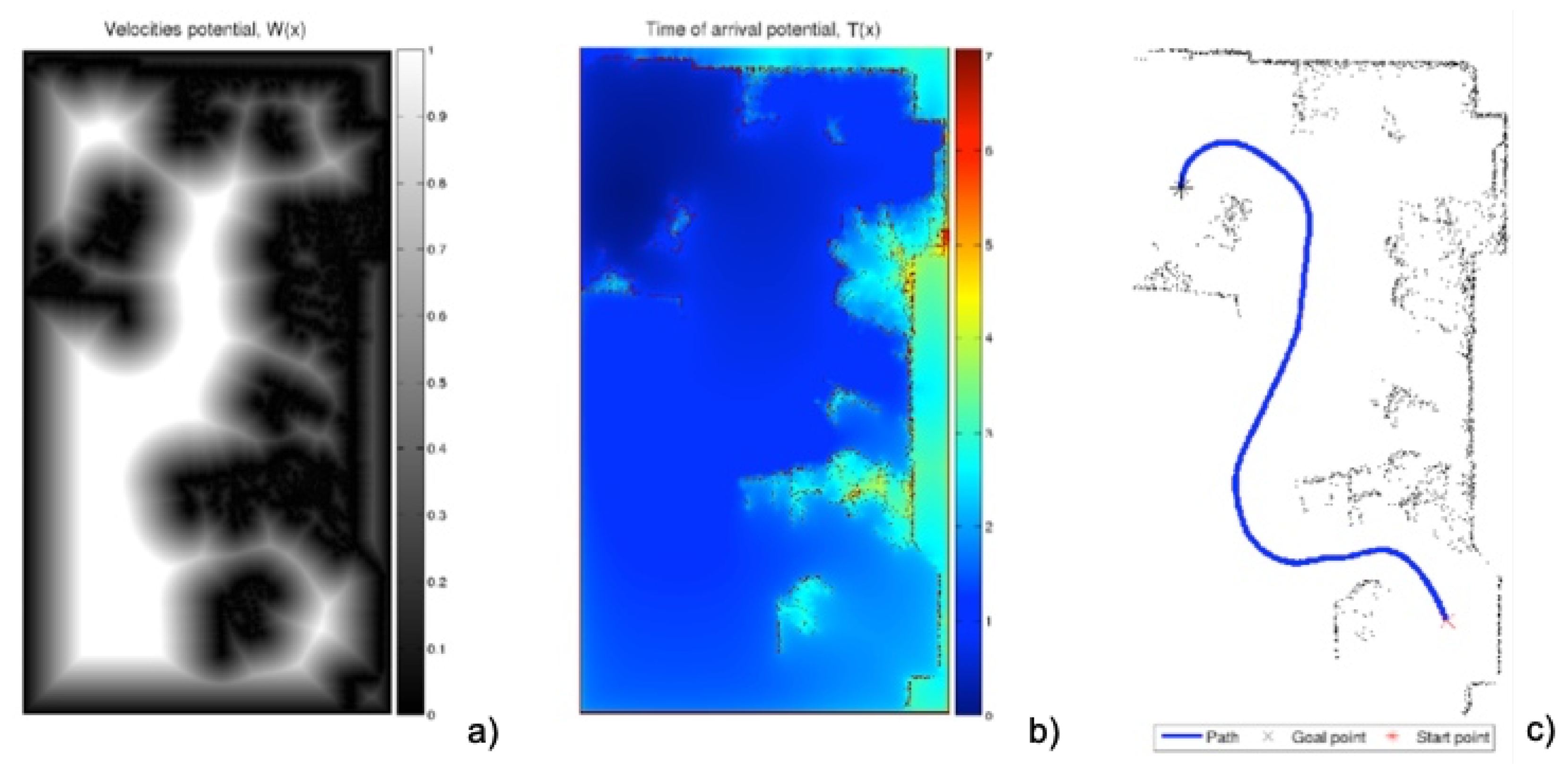
2.1. and Methods
| Algorithm 1 Fast Marching Method |
| Require: A grid map X of size , source point . |
| Ensure: The grid map X with the T value set for all cells. |
| Initialization. |
|
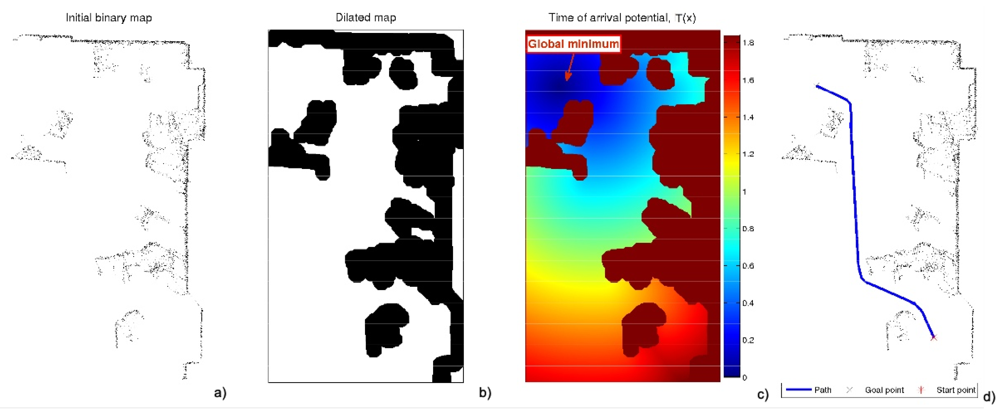
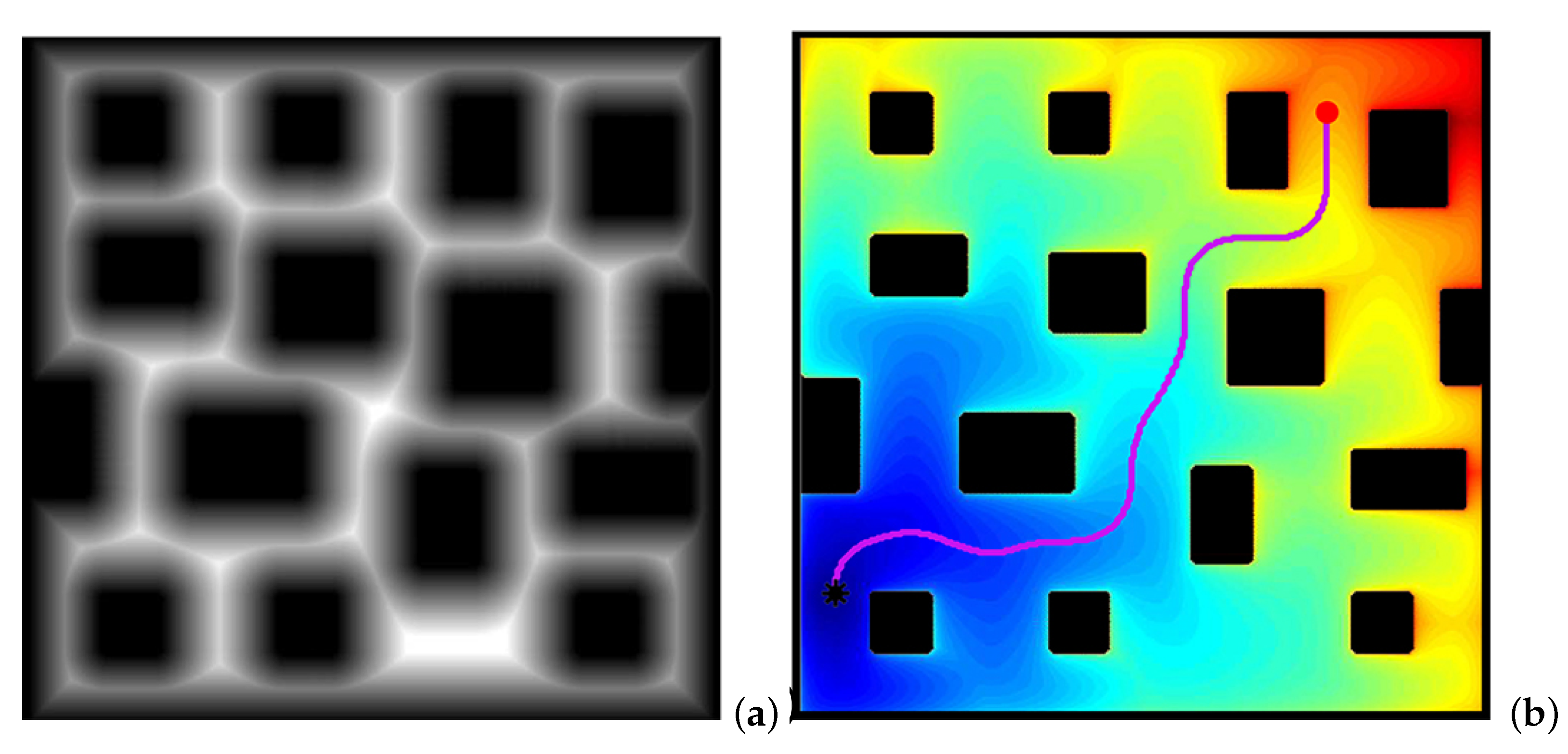
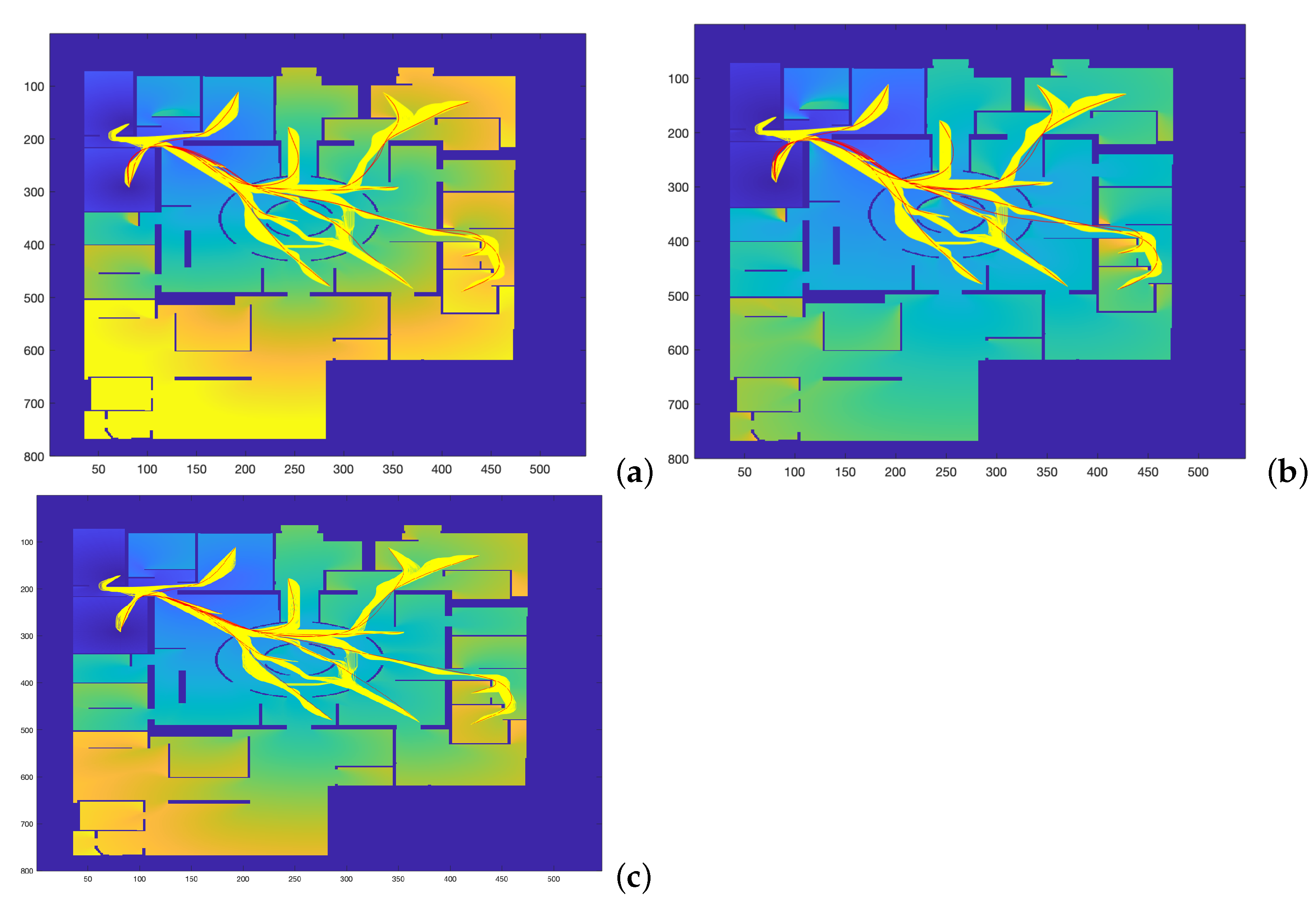
- The first is the saturation parameter , which consists of setting a maximum value, between 0 and 1, from which all the values of the matrix W are equal to 1.In Figure 3 and Figure 4, for = 0.8 and = 0.6, respectively, it can be seen that the white area away from obstacles is more or less large. A saturation value closer to zero implies less curved trajectories, but with more angle at certain points and closer to obstacles. The trajectory of Figure 3c) also presents a curvature in some points bigger than that of Figure 4c).
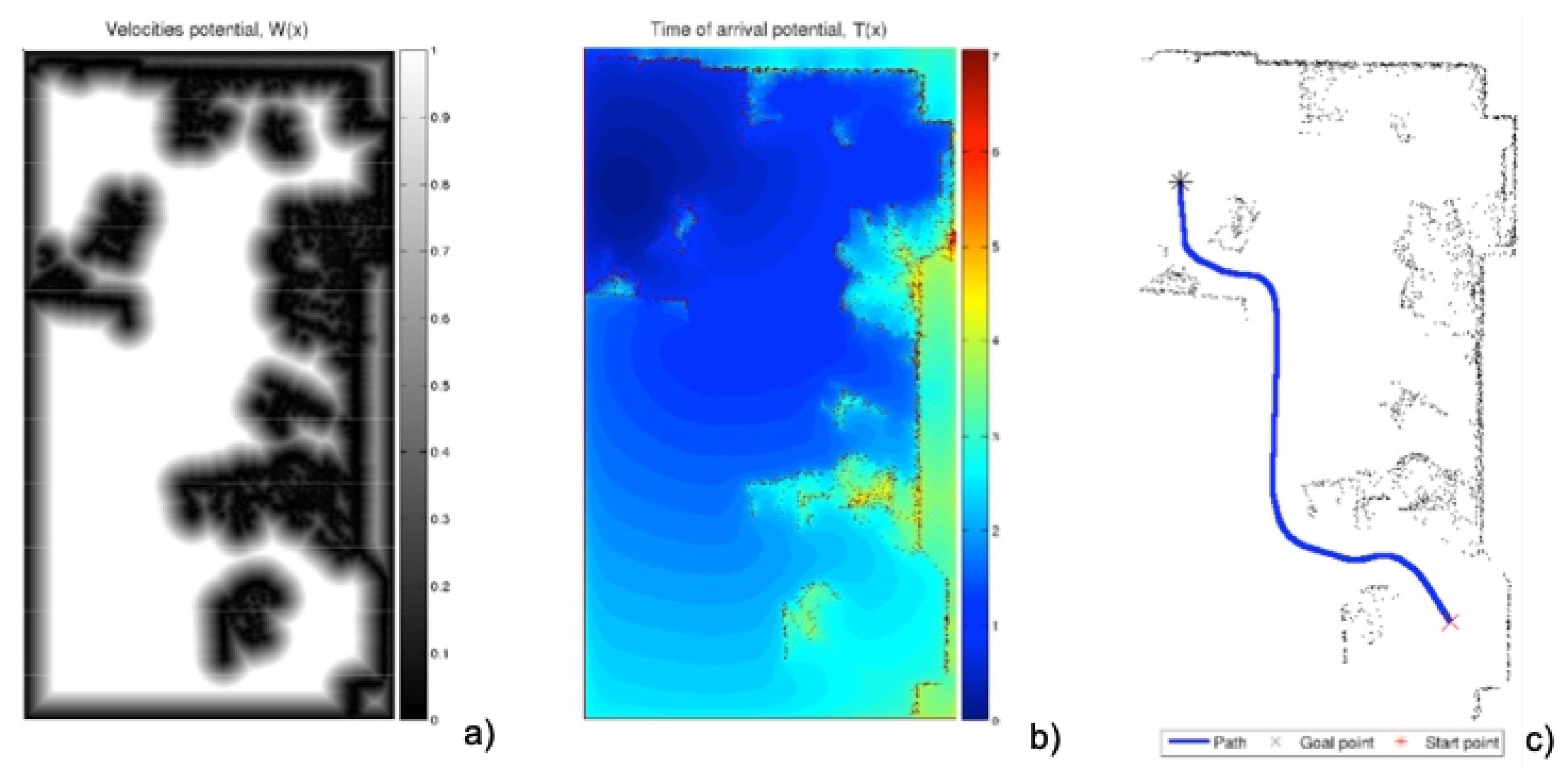
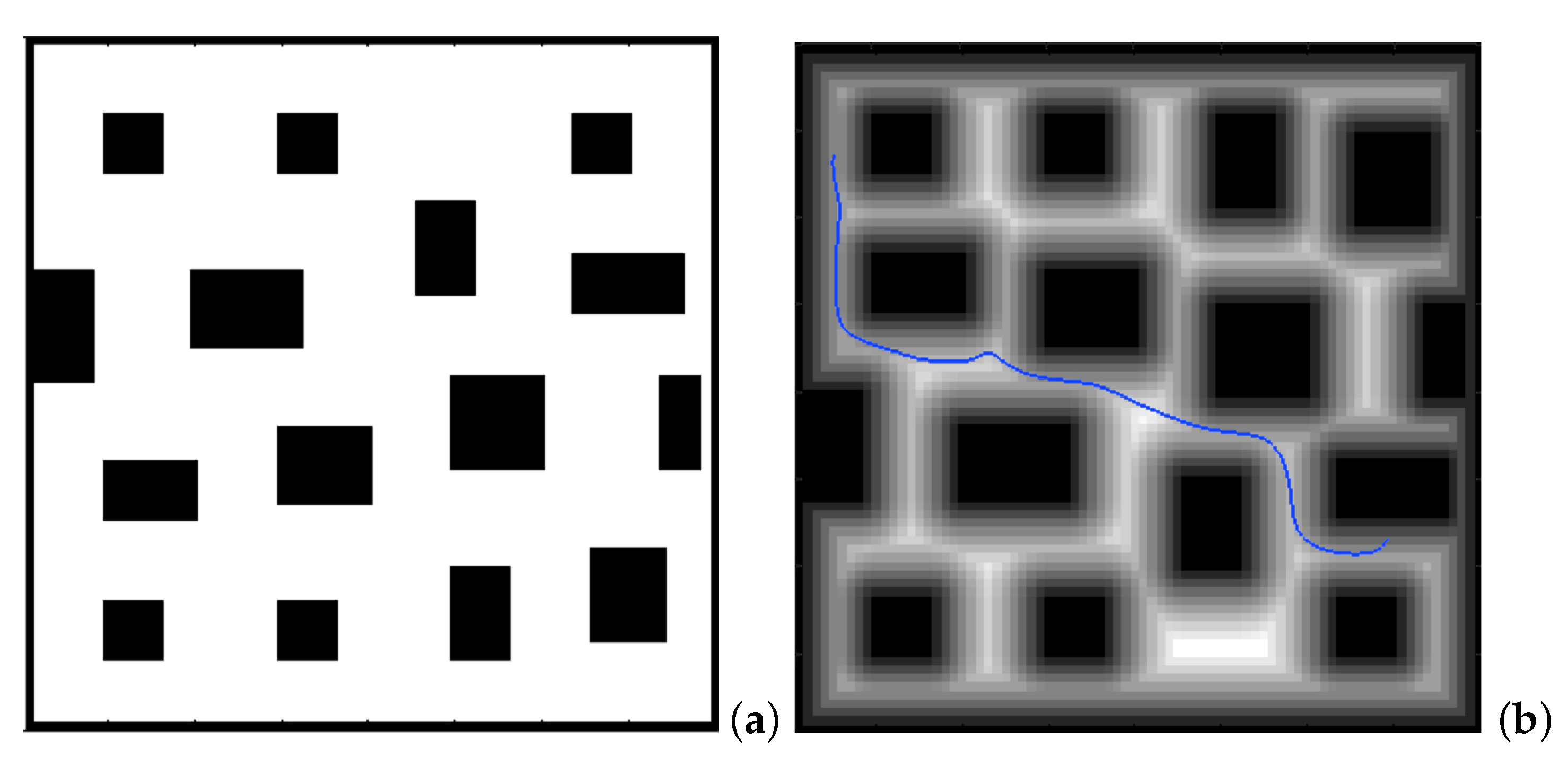
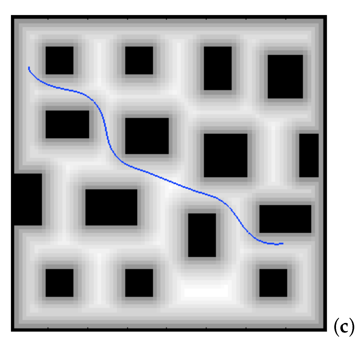
- The second parameter, , is an exponent between 0 and 1 to which each coefficient of matrix W of the first potential is raised. Figure 5 and Figure 6 show the behaviour of the algorithm for varying values of . The closer the exponent to zero, the clearer the image and the less curvature of the trajectories. The closer the exponent to one, the more similar the curvature to the Medial Axis Transform (MAT), although the smoother the trajectories and the more separated from obstacles (safer paths).It is also possible to raise each coefficient of the matrix to numbers greater than one, but the results are not of interest because they are more and more similar to the trajectories obtained with a Voronoi diagram that have sharp edges.
2.2. Dubins, Euler–Mumford Elastica and Reeds–Shepp methods
3. Discussion of Simulation Results
3.1. Simulation Execution Conditions
- 1.
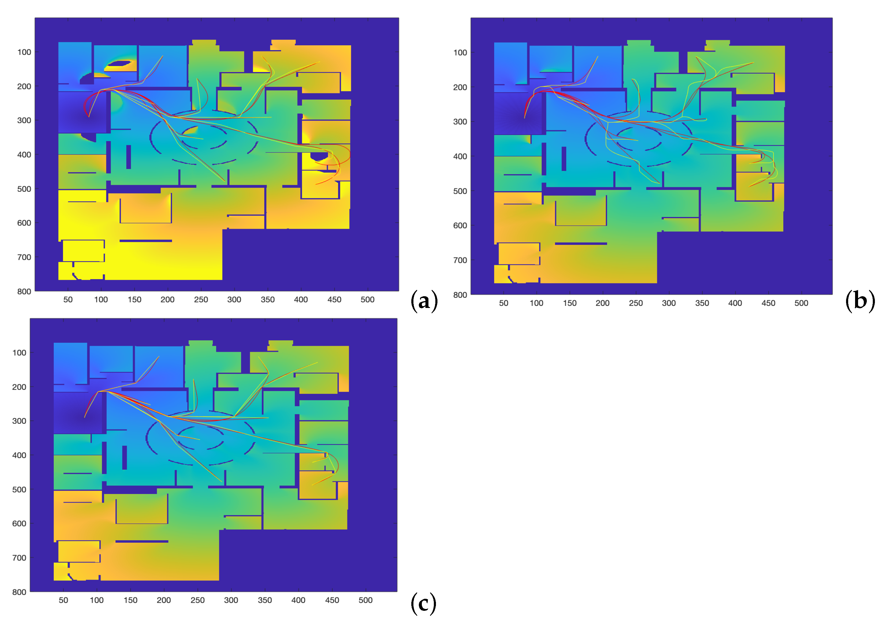
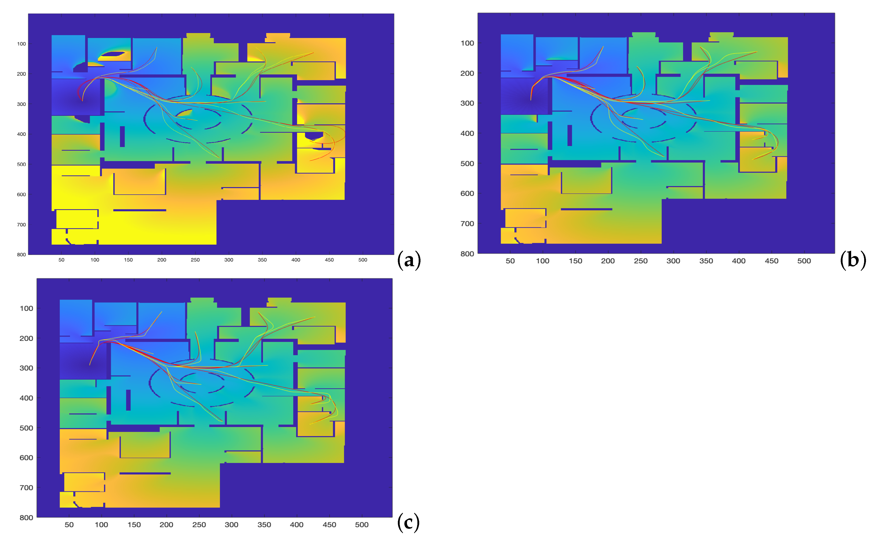
- The map in Figure 7, corresponding to the city area of the Centre Pompidou, is used for the simulations.
- 2.
- A total of 24 different trajectories are executed by each method, covering the main central area of the map.
- 3.
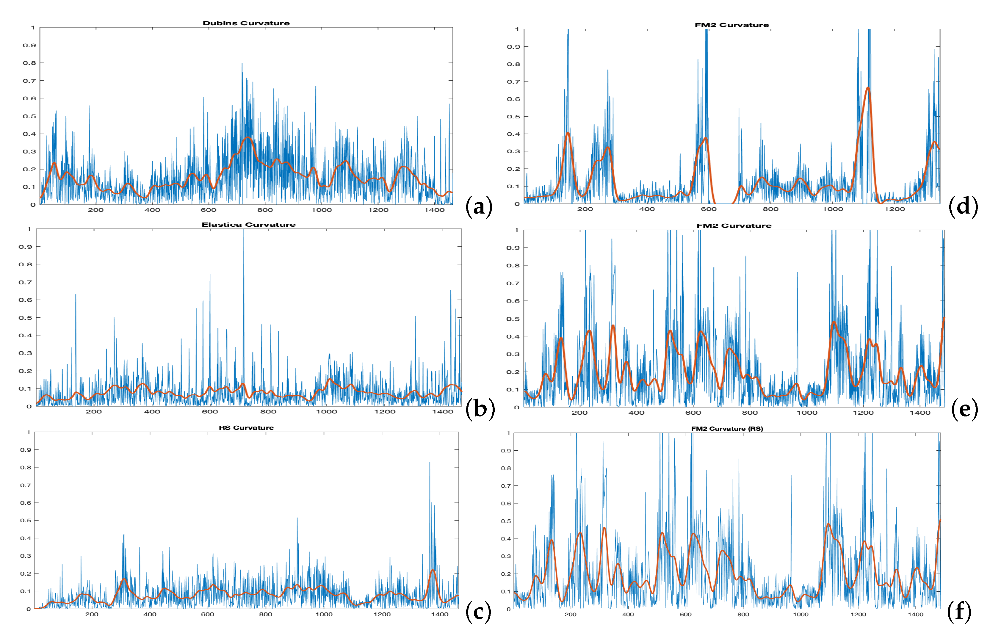
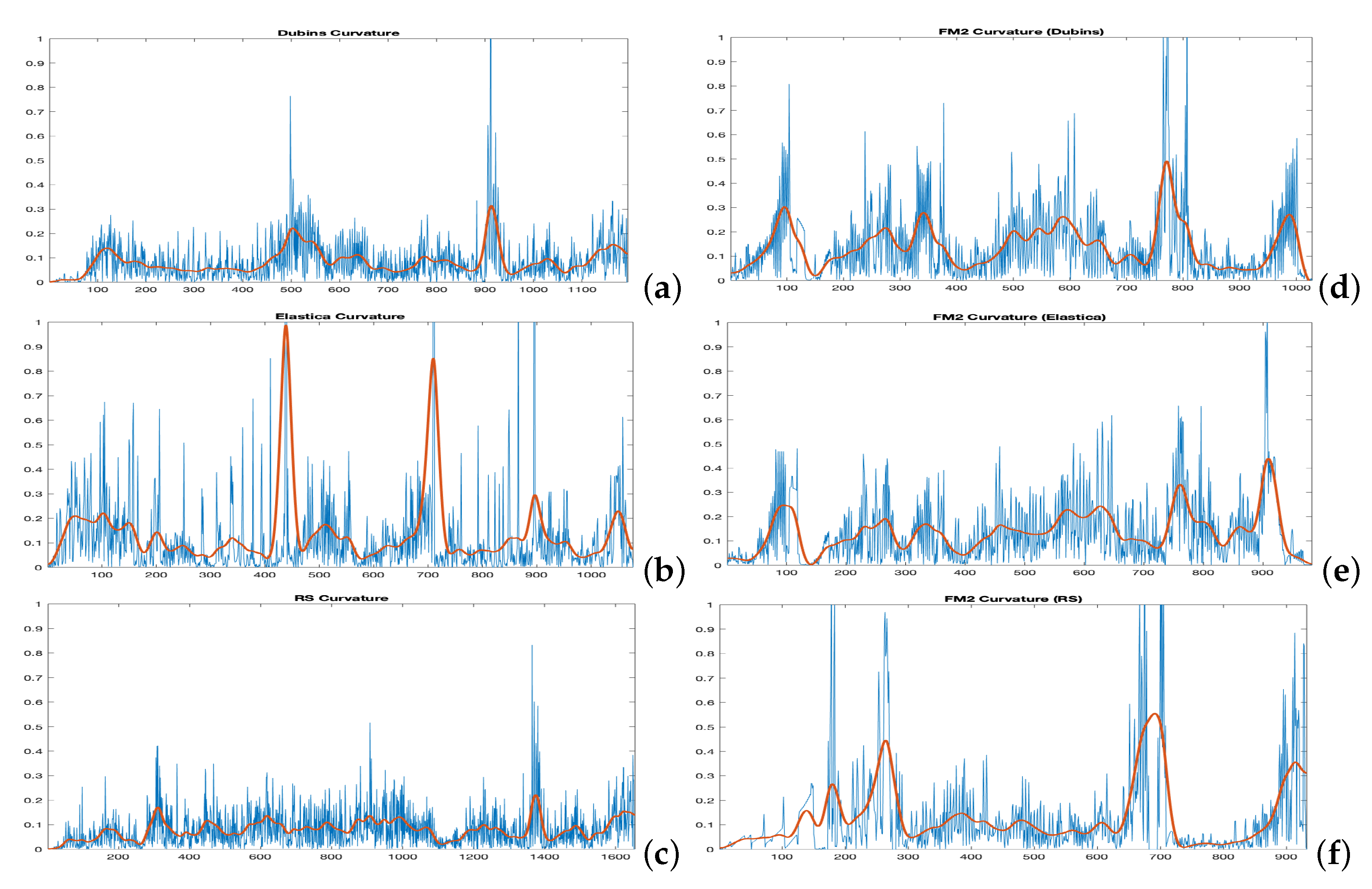
- For the execution of the Dubins car, the Euler–Mumford Elastica and the Reeds–Shepp approaches, the codes proposed in [26,27] by Mirebeau et al. are used, which apply the Fast Marching with stencils method (see Section 2.2 and Equations (4) and (5) for a detailed description of the curvature cost functions). The initial and end points of the 24 trajectories are specified, and parameter is taken as 1.
- 4.
- The method is applied using the same initial and end points defined before, varing parameters and as described in the following subsection.
- 5.
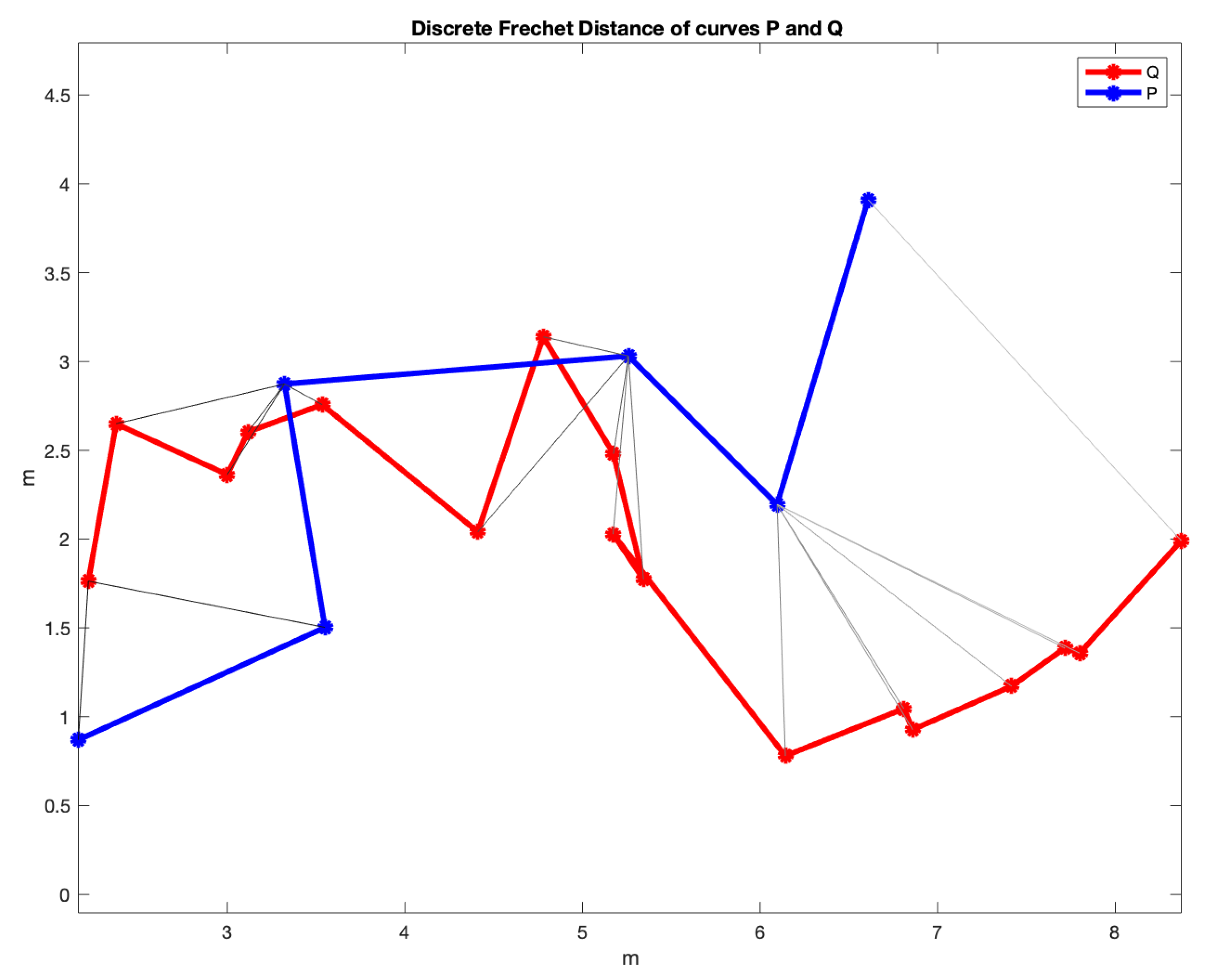
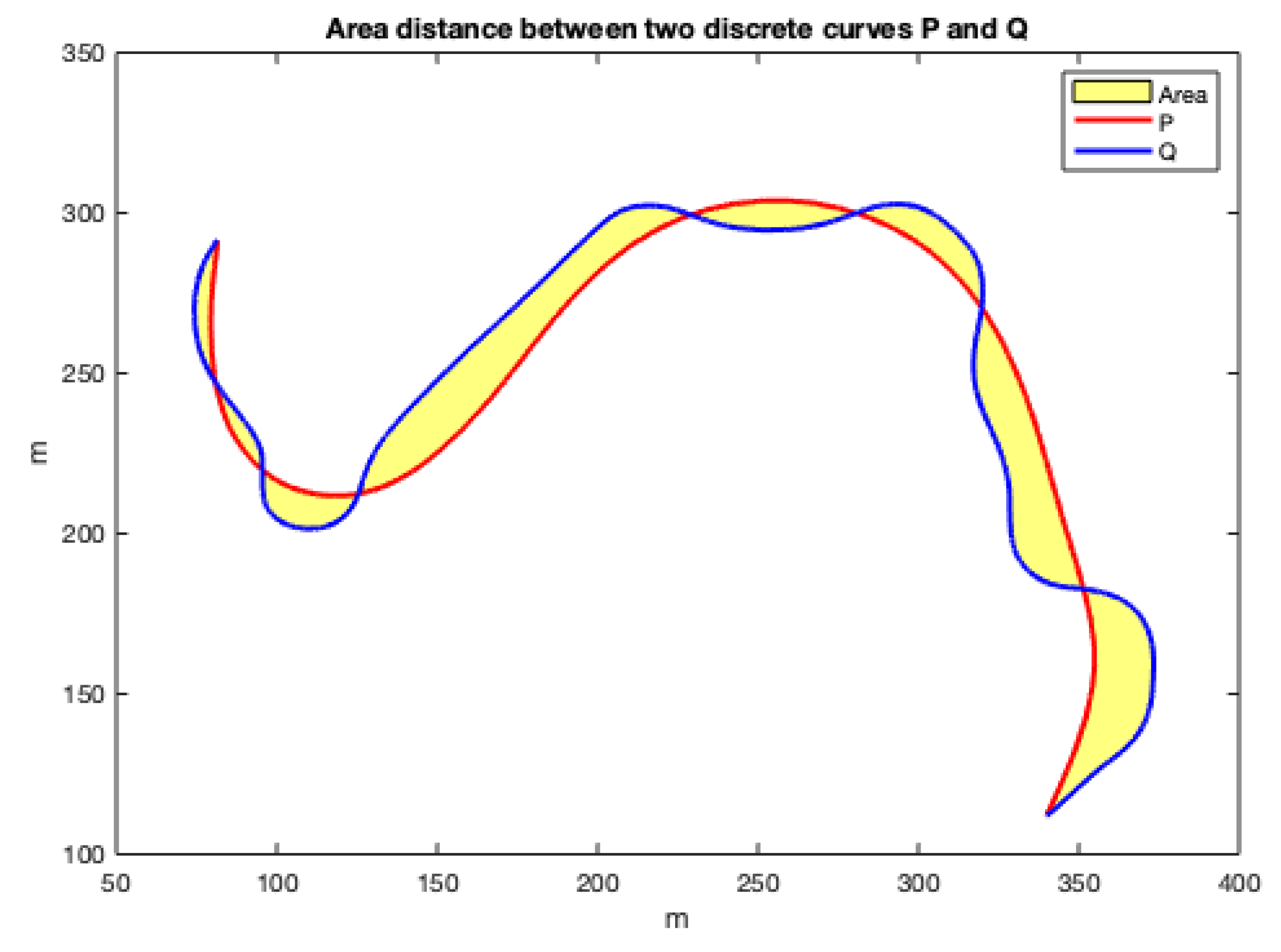
- For the sake of comparison of the resulting paths and their curvatures using these four methods, two measures of similarity will be used: the Fréchet distance and the area between two curves, as defined before. The results are given and discussed in the following subsections.

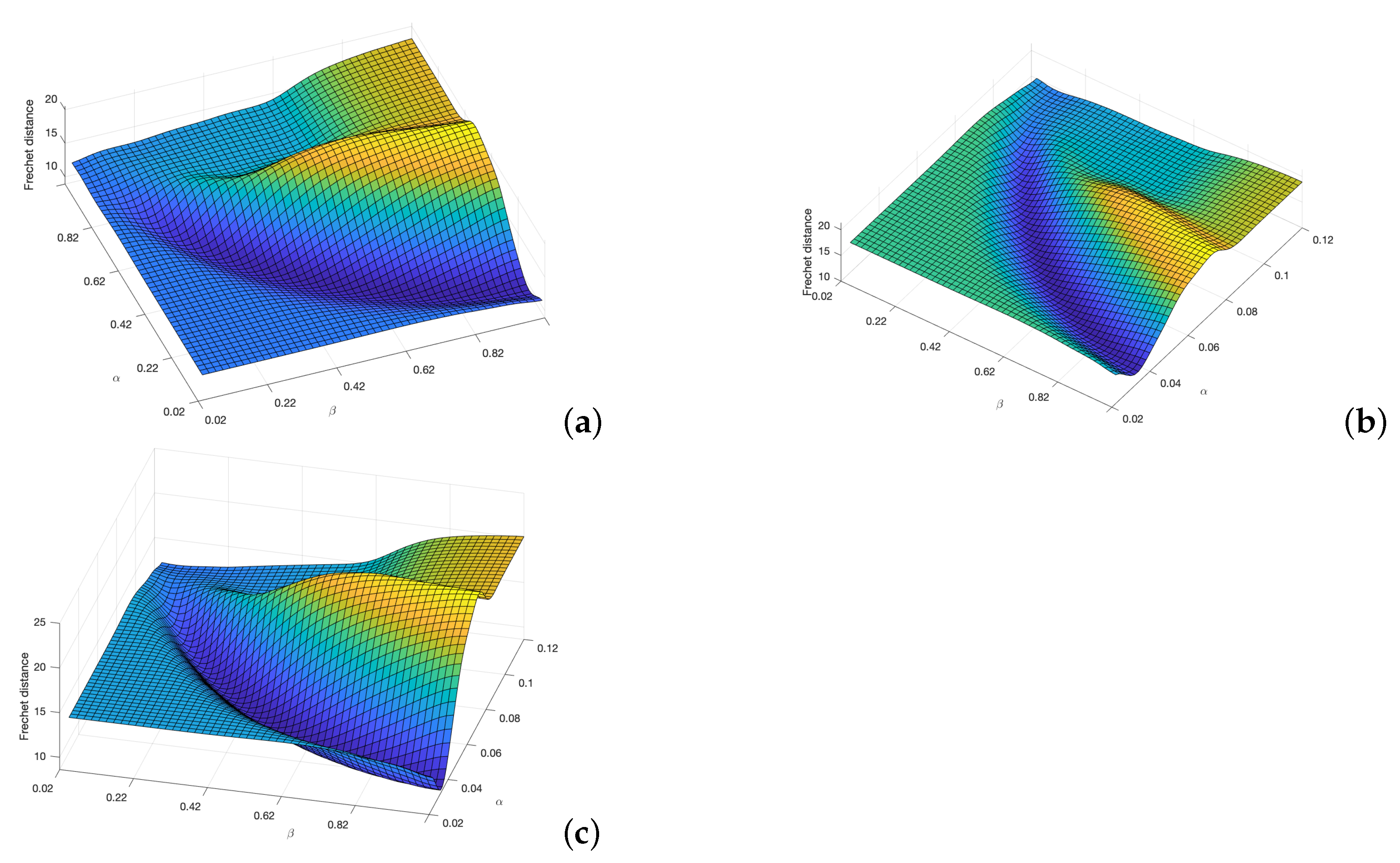
3.2. Minimization of the Fréchet Distance
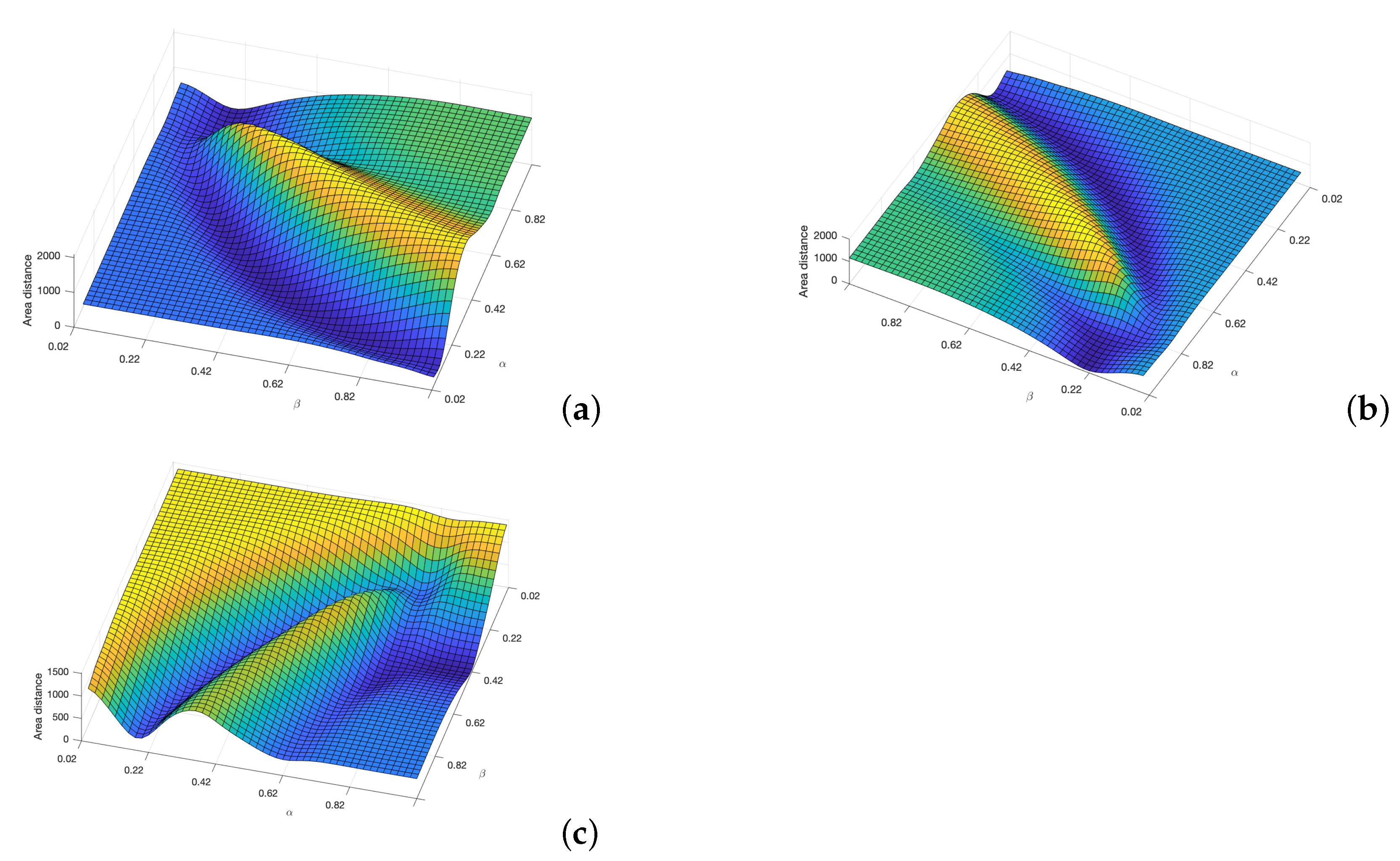
3.3. Minimization of the Area between Curves
3.4. Distance from Paths to Obstacles
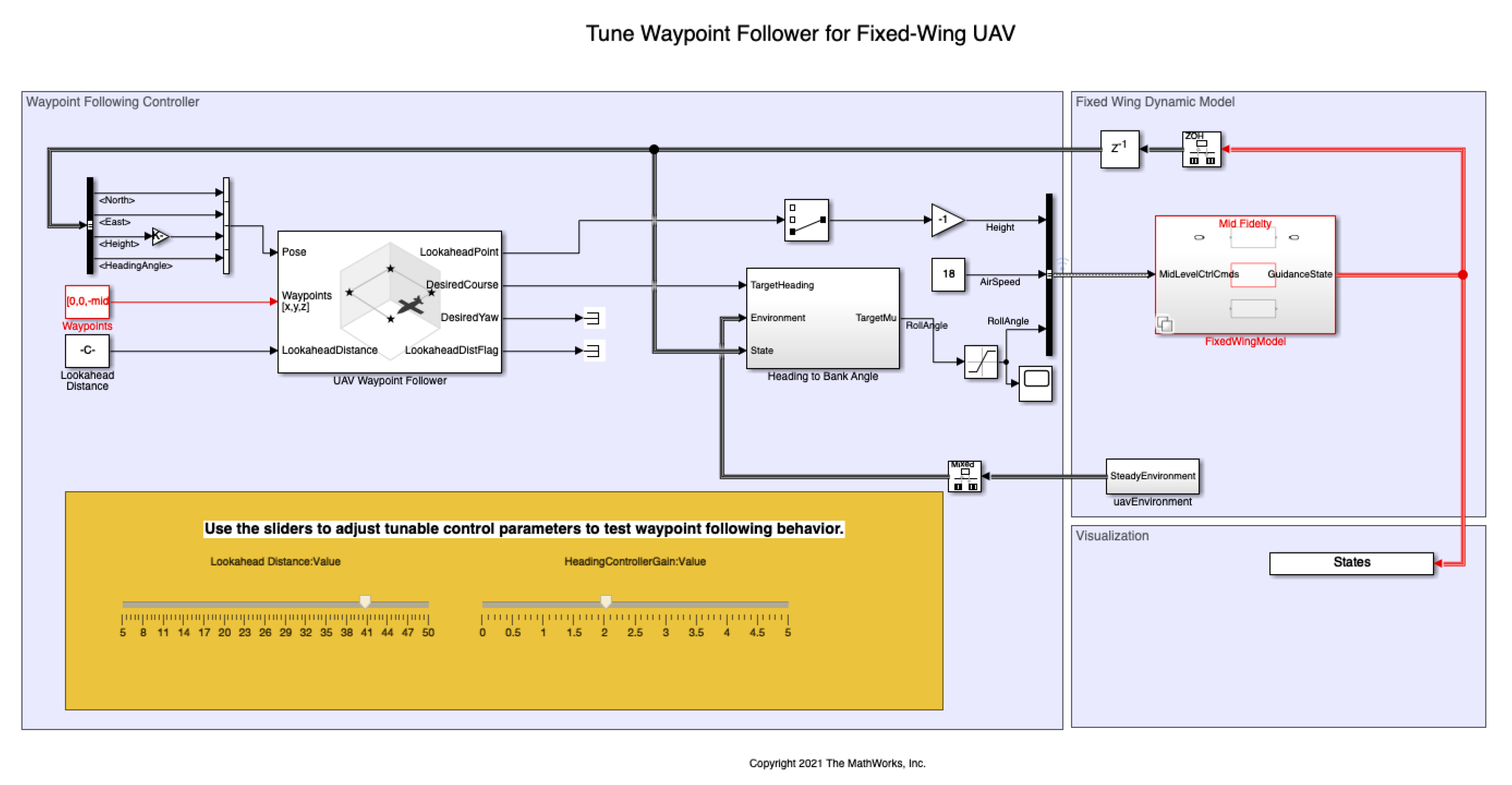
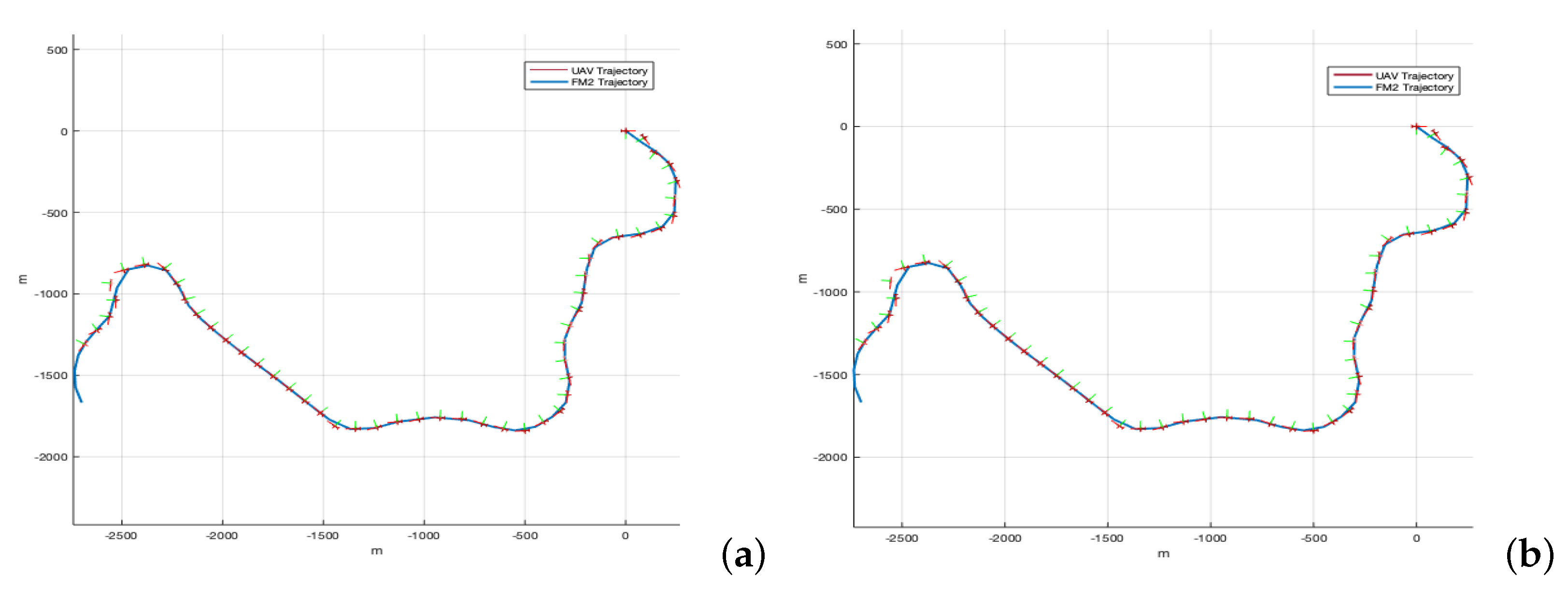
3.5. Simulation Results Using a Quadcopter Model and a Fixed-Wing UAV
4. Conclusions
Author Contributions
Funding
Institutional Review Board Statement
Informed Consent Statement
Data Availability Statement
Conflicts of Interest
References
- LaValle, S. Planning Algorithms Cambridge; Cambridge University Press: Cambridge, UK, 2006. [Google Scholar]
- Dijkstra, E. A Note on Two Problems in Connection with Graphs. Numer. Math. 1959, 1, 269–271. [Google Scholar] [CrossRef] [Green Version]
- Hart, P.; Nilsson, N.; Raphael, B. A Formal Basis for the Heuristic Determination of Minimum Cost Paths. Syst. Sci. Cybern. 1968, 4, 100–107. [Google Scholar] [CrossRef]
- Kavraki, L.; Svestka, P.; Latombe, J.; Overmars, M. Probabilistic roadmaps for path planning in high-dimensional configuration spaces. IEEE Trans. Robot. Autom. 1996, 12, 566–580. [Google Scholar] [CrossRef] [Green Version]
- Yan, Z.; Zhao, Y.; Chen, T.; Deng, C. 3D path planning for AUV based on circle searching. In Proceedings of the OCEANS 2012 MTS/IEEE: Harnessing the Power of the Ocean, Hampton Roads, VA, USA, 14–19 October 2012. [Google Scholar]
- Pivtoraiko, M.; Kelly, A. Generating near minimal spanning control sets for constrained motion planning in discrete state spaces. In Proceedings of the 2005 IEEE/RSJ International Conference on Intelligent Robots and Systems (IROS), Edmonton, AB, Canada, 2–6 August 2005; pp. 594–600. [Google Scholar]
- Dolgov, D.; Thrun, S.; Montemerlo, M.; Diebel, J. Practical search techniques in path planning for autonomous driving. Int. Symp. Comb. Search SoCS 2008, 1001, 18–80. [Google Scholar]
- LaValle, S.; Kuffner, J. Randomized kinodynamic planning. Int. J. Robot. Res. 2001, 20, 378–400. [Google Scholar] [CrossRef]
- Dubins, L.E. On Curves of Minimal Length with a Constraint on Average Curvature, and with Prescribed Initial and Terminal Positions and Tangents. Am. J. Math. 1957, 79, 497–516. [Google Scholar] [CrossRef]
- Hernández, J.; Vidal, E.; Moll, M.; Palomeras, N.; Carreras, M.; Kavraki, L. Online motion planning for unexplored underwater environments using autonomous underwater vehicles. J. Field Robot. 2019, 36, 370–396. [Google Scholar] [CrossRef]
- Pairet, E.; Hernández, J.D.; Lahijanian, M.; Carreras, M. Uncertainty-based Online Mapping and Motion Planning for Marine Robotics Guidance. In Proceedings of the IEEE International Conference on Intelligent Robots and Systems, Madrid, Spain, 1–5 October 2018; pp. 2367–2374. [Google Scholar]
- Gundlach, I.; Konigorski, U.; Hoedt, J. Zeitoptimale Trajektorienplanung für automatisiertesFahren im fahrdynamischen Grenzbereich. VDI Ber. 2017, 2292, 223–234. [Google Scholar]
- Perantoni, G.; Limebeer, D.J. Optimal control for a formula one car with variable parameters. Veh. Syst. Dyn. 2014, 52, 653–678. [Google Scholar] [CrossRef] [Green Version]
- Heilmeier, A.; Wischnewski, A.; Hermansdorfer, L.; Betz, J.; Lienkamp, M.; Lohmann, B. Minimum curvature trajectory planning and control for an autonomous race car. J. Veh. Syst. Dynam. 2020, 58, 1497–1527. [Google Scholar] [CrossRef]
- López, B. Path Planning and Collision Risk Management Strategy for Multi-UAV Systems in 3D Environments. Sensors 2021, 21, 4414. [Google Scholar] [CrossRef] [PubMed]
- Levien, R. The Elastica: A Mathematical History. In Technical Report UCB/EECS-2008-103; EECS Department, University of California: Berkeley, CA, USA, 2008. [Google Scholar]
- Oldfather, W.A.; Ellis, C.A.; Brown, D.M. Leonhard Euler’s Elastic Curves. Isis 1933, 20, 72–160. [Google Scholar] [CrossRef]
- Reeds, J.; Shepp, L. Optimal paths for a car that goes both forwards and backwards. Pac. J. Math. 1990, 145, 367–393. [Google Scholar] [CrossRef] [Green Version]
- Alt, H.; Godau, M. Computing the Fréchet distance between two polygonal curves. Int. J. Comput. Geom. Appl. 1995, 5, 75–91. [Google Scholar] [CrossRef]
- Sethian, J.A. A fast marching level set method for monotonically advancing fronts. Proc. Natl. Acad. Sci. USA 1996, 93, 1591–1595. [Google Scholar] [CrossRef] [PubMed] [Green Version]
- Sethian, J. Level Set Methods: Evolving Interfaces in Computational Geometry, Fluid Mechanics, Computer Vision, and Materials Science. In Cambridge Monographs on Applied and Computational Mathematics; Cambridge University Press: Cambridge, UK, 1996. [Google Scholar]
- Gómez, J.V.; Álvarez, D.; Garrido, S.; Moreno, L. Fast Methods for Eikonal Equations: An Experimental Survey. IEEE Access 2019, 7, 39005–39029. [Google Scholar] [CrossRef]
- Garrido, S.; Moreno, L.; Blanco, D. Voronoi Diagram and Fast Marching applied to Path Planning. In Proceedings of the 2006 IEEE International Conference on Robotics and Automation, Orlando, FL, USA, 15–19 May 2006; pp. 3049–3054. [Google Scholar]
- Garrido, S.; Moreno, L.; Abderrahim, M.; Blanco, D. FM2: A real-time sensor-based feedback controller for mobile robots. Int. J. Robot. Autom. 2009, 24, 48–65. [Google Scholar]
- Valero-Gomez, A.; Gomez, J.V.; Garrido, S.; Moreno, L. The Path to Efficiency: Fast Marching Method for Safer, More Efficient Mobile Robot Trajectories. IEEE Robot. Autom. Mag. 2013, 20, 111–120. [Google Scholar] [CrossRef] [Green Version]
- Mirebeau, J.M.; Portegies, J. Hamiltonian Fast Marching: A Numerical Solver for Anisotropic and Non-Holonomic Eikonal PDEs. Image Process. Line 2019, 9, 47–93. [Google Scholar] [CrossRef]
- Mirebeau, J.M. Fast Marching methods for Curvature Penalized Shortest Paths. J. Math. Imag. Vision. 2018, 60, 784–815. [Google Scholar] [CrossRef] [Green Version]
- García, D. A fast all-in-one method for automated post-processing of PIV data. Exp. Fluids 2011, 50, 1247–1259. [Google Scholar] [CrossRef] [PubMed]
- Matlab. Transition from Low to High-Fidelity UAV Models in Three Stages. 2022. Available online: https://es.mathworks.com/help/uav/ug/transition-from-low-to-high-fidelity-uav-models.html (accessed on 1 January 2022).


| Dubins | Euler–Mumford Elastica | Reeds–Shepp | ||
|---|---|---|---|---|
| Computation time (secs) | 18.936 | 19.199 | 19.577 | 0.087 |
| Dubins | Euler–Mumford Elastica | Reeds–Shepp | |
|---|---|---|---|
| 0.1 | 0.3 | 0.038 | |
| 0.98 | 0.96 | 0.92 | |
| Fréchet cost function | 8.1 | 11.1 | 9.2 |
| Dubins | Euler–Mumford Elastica | Reeds–Shepp | |
|---|---|---|---|
| 0.90 | 0.84 | 0.40 | |
| 0.18 | 0.20 | 0.50 | |
| Area cost function | 4.50 | 2.19 | 0.3352 |
| Dubins | Euler–Mumford Elastica | Reeds–Shepp | |
|---|---|---|---|
| 0.90 | 0.84 | 0.40 | |
| 0.18 | 0.20 | 0.50 | |
| Original distance | 0.0093 | 0.0169 | 0.0071 |
| Distance of the approximation | 0.0276 | 0.0191 | 0.0214 |
Publisher’s Note: MDPI stays neutral with regard to jurisdictional claims in published maps and institutional affiliations. |
© 2022 by the authors. Licensee MDPI, Basel, Switzerland. This article is an open access article distributed under the terms and conditions of the Creative Commons Attribution (CC BY) license (https://creativecommons.org/licenses/by/4.0/).
Share and Cite
Garrido, S.; Muñoz, J.; López, B.; Quevedo, F.; Monje, C.A.; Moreno, L. FM2 Path Planner for UAV Applications with Curvature Constraints: A Comparative Analysis with Other Planning Approaches. Sensors 2022, 22, 3174. https://doi.org/10.3390/s22093174
Garrido S, Muñoz J, López B, Quevedo F, Monje CA, Moreno L. FM2 Path Planner for UAV Applications with Curvature Constraints: A Comparative Analysis with Other Planning Approaches. Sensors. 2022; 22(9):3174. https://doi.org/10.3390/s22093174
Chicago/Turabian StyleGarrido, Santiago, Javier Muñoz, Blanca López, Fernando Quevedo, Concepción A. Monje, and Luis Moreno. 2022. "FM2 Path Planner for UAV Applications with Curvature Constraints: A Comparative Analysis with Other Planning Approaches" Sensors 22, no. 9: 3174. https://doi.org/10.3390/s22093174
APA StyleGarrido, S., Muñoz, J., López, B., Quevedo, F., Monje, C. A., & Moreno, L. (2022). FM2 Path Planner for UAV Applications with Curvature Constraints: A Comparative Analysis with Other Planning Approaches. Sensors, 22(9), 3174. https://doi.org/10.3390/s22093174