Seabed Modelling by Means of Airborne Laser Bathymetry Data and Imbalanced Learning for Offshore Mapping

Abstract

An important problem associated with the aerial mapping of the seabed is the precise classification of point clouds characterizing the water surface, bottom, and bottom objects. This study aimed to improve the accuracy of classification by addressing the asymmetric amount of data representing these three groups. A total of 53 Synthetic Minority Oversampling Technique (SMOTE) algorithms were adjusted and evaluated to balance the amount of data. The prepared data set was used to train the Multi-Layer Perceptron (MLP) neural network used for classifying the point cloud. Data balancing contributed to significantly increasing the accuracy of classification. The best overall classification accuracy achieved varied from 95.8% to 97.0%, depending on the oversampling algorithm used, and was significantly better than the classification accuracy obtained for unbalanced data and data with downsampling (89.6% and 93.5%, respectively). Some of the algorithms allow for 10% increased detection of points on the objects compared to unbalanced data or data with simple downsampling. The results suggest that the use of selected oversampling algorithms can aid in improving the point cloud classification and making the airborne laser bathymetry technique more appropriate for seabed mapping.

1. Introduction

Information on water depth and seabed topography can contribute to improving the safety of maritime transport and to the development of other maritime industries, including the offshore sector. Hydrographic surveying is done systematically all over the world to prepare data for nautical charts, electronic navigation systems, and other databases used in the management of hydrospace and maritime infrastructure. The airborne laser bathymetry (ALB) technique can be a valuable addition to Multibeam Echosounders (MBES) or perhaps an alternative in shallow waters. It has proven to be a large-scale, accurate, rapid, safe, and versatile approach for surveying shallow waters and coastlines where sonar systems are ineffective or impossible to use [1,2,3,4]. Research has shown that ALB can identify similar seafloor features such as MBES systems [5]. However, additional improvements must be done to separate the LiDAR seafloor intensity data from the depth component of the signal waveform. Receiving bathymetric lidar data with unassigned point classes or inaccurate point classification that may not meet industrial or research requirements is not unusual [6]. Studies that have used ALB for depth determination and object detection primarily point to challenges in classifying the resulting point cloud into three basic groups: bottom, water surface, and bottom objects. These issues can be overcome using well-recognized machine learning classification methods.

The main goal of this study is to increase the accuracy of the classification of point clouds measured by an ALB scanner to improve seabed modeling and object detection.

This paper can be considered a novel input to the ALB classification of point clouds with the use of imbalanced learning. To achieve the goal, the study evaluated Multi-Layer Perceptron (MLP) Artificial Neural Network (ANN) with the softmax activation function employing over 50 variants of the oversampling techniques for imbalanced learning. The results confirmed that data balancing had a quantitative impact on classification accuracy, allowing enhanced detection of seabed and bottom based on the ALB data. The classification results indicated that the best overall classification accuracy achieved varied from 95.8% to 97.0% depending on the oversampling algorithm used and was significantly better than the classification accuracy obtained for unbalanced data and data with downsampling (89.6% and 93.5%, respectively). Some of the algorithms allow for 10% increased detection of points on the objects compared to unbalanced data or data with simple downsampling. This study did not develop a new data balancing method or enhance the existing ones.

The classification accuracy of point clouds of all the classes is influenced by class distribution. According to the scanned area in the majority, the laser scanning data are unbalanced, and therefore require remodeling. The ALB data set of shallow waters comprises data on the seabed and a small percentage of data on underrepresented seabed objects. This application necessitates a high rate of accurate detection in the minority class (seabed objects) and a low rate of mistakes in the majority class (seabed or water surface). Different oversampling methods have been analyzed to address this concern [7]. Archaeologists focusing on detecting former field systems from LiDAR data in their research recommend the use of the Synthetic Minority Oversampling Technique (SMOTE) for achieving better results [8]. Balancing the training data for automatic mapping of high-voltage power lines based on the LiDAR data led to an almost 10% increase in accuracy in comparison to imbalanced data [9]. Landslide prediction research based on a set of geomorphological factors revealed that the Support Vector Machine (SVM) model yielded the highest accuracy with the SMOTE data balancing method [10]. The supporting synthetic samples were used in the classification of bottom materials (sand, stones, rocks) performed using ALB. The obtained results were promising but were specific for particular classes [11]. A study on the application of SMOTE for balancing data distribution with land cover mapping using LiDAR data showed increased detection accuracy. The challenges associated with imbalanced classes and low density of LiDAR point clouds in urban areas were also satisfactorily resolved by applying several oversampling methods for the classification and extraction of roof superstructures [12]. Due to its proven advantages in classification, the present study used SMOTE, a method for producing synthetic new data from existing ones, which provided new information and variations to synthetically generated data.

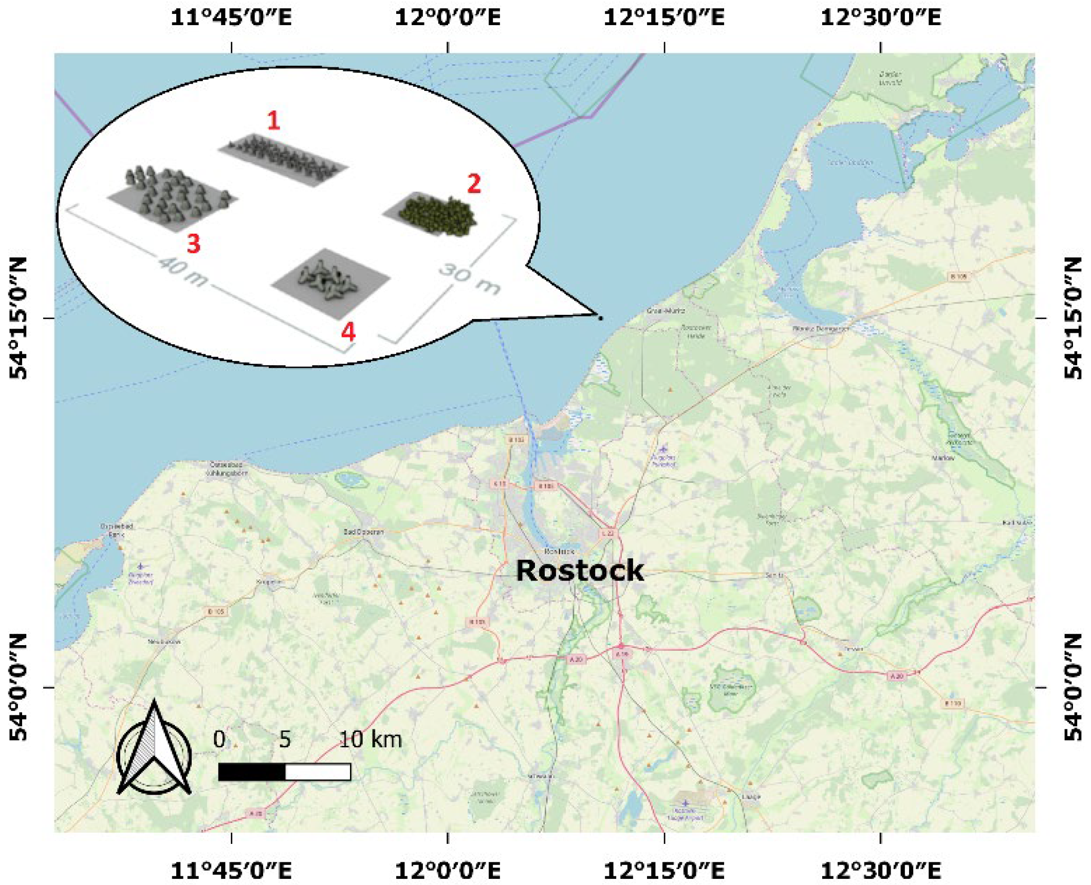
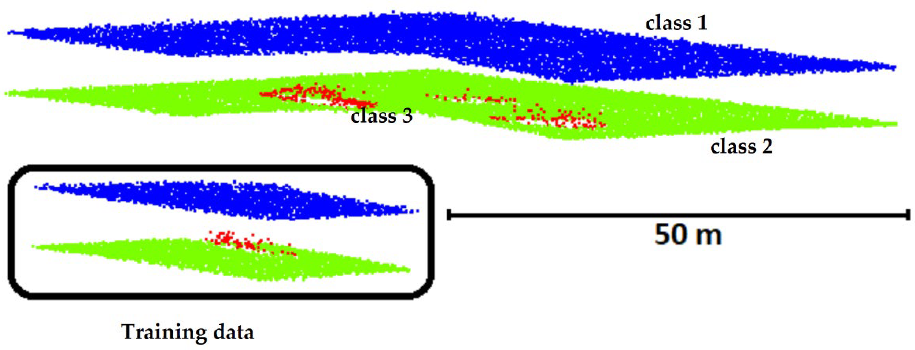
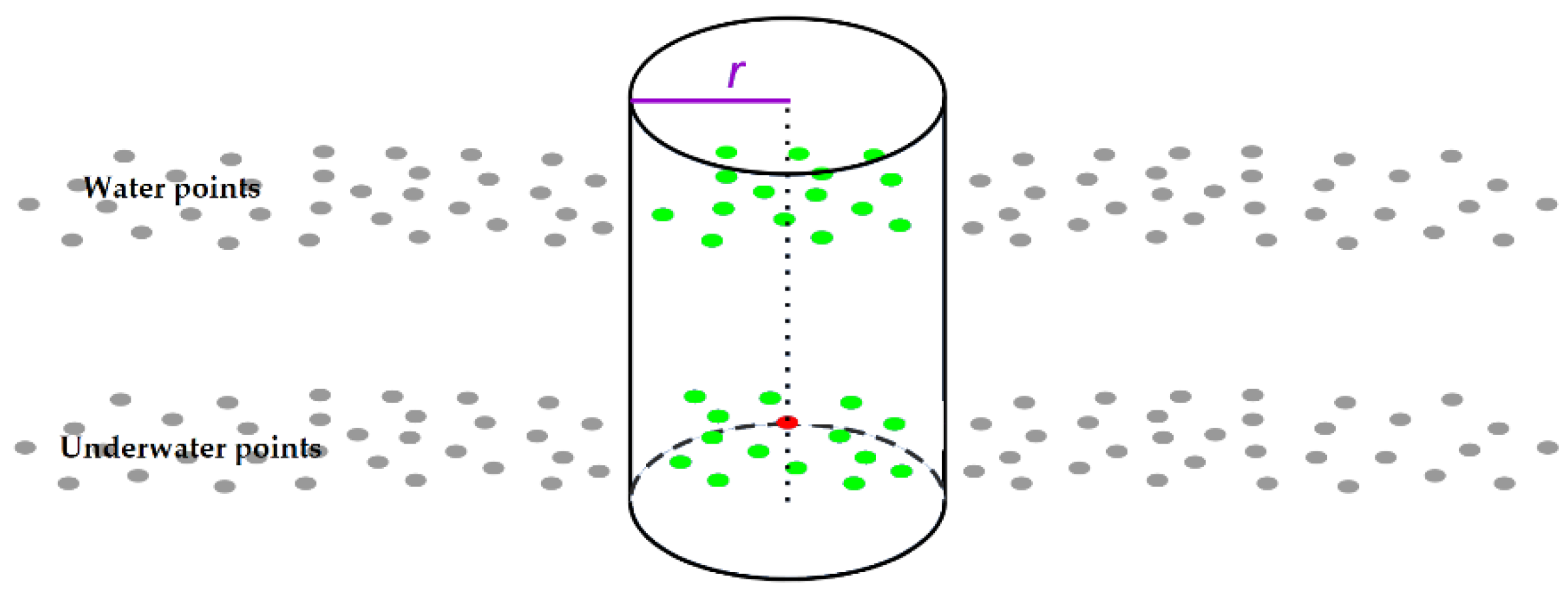
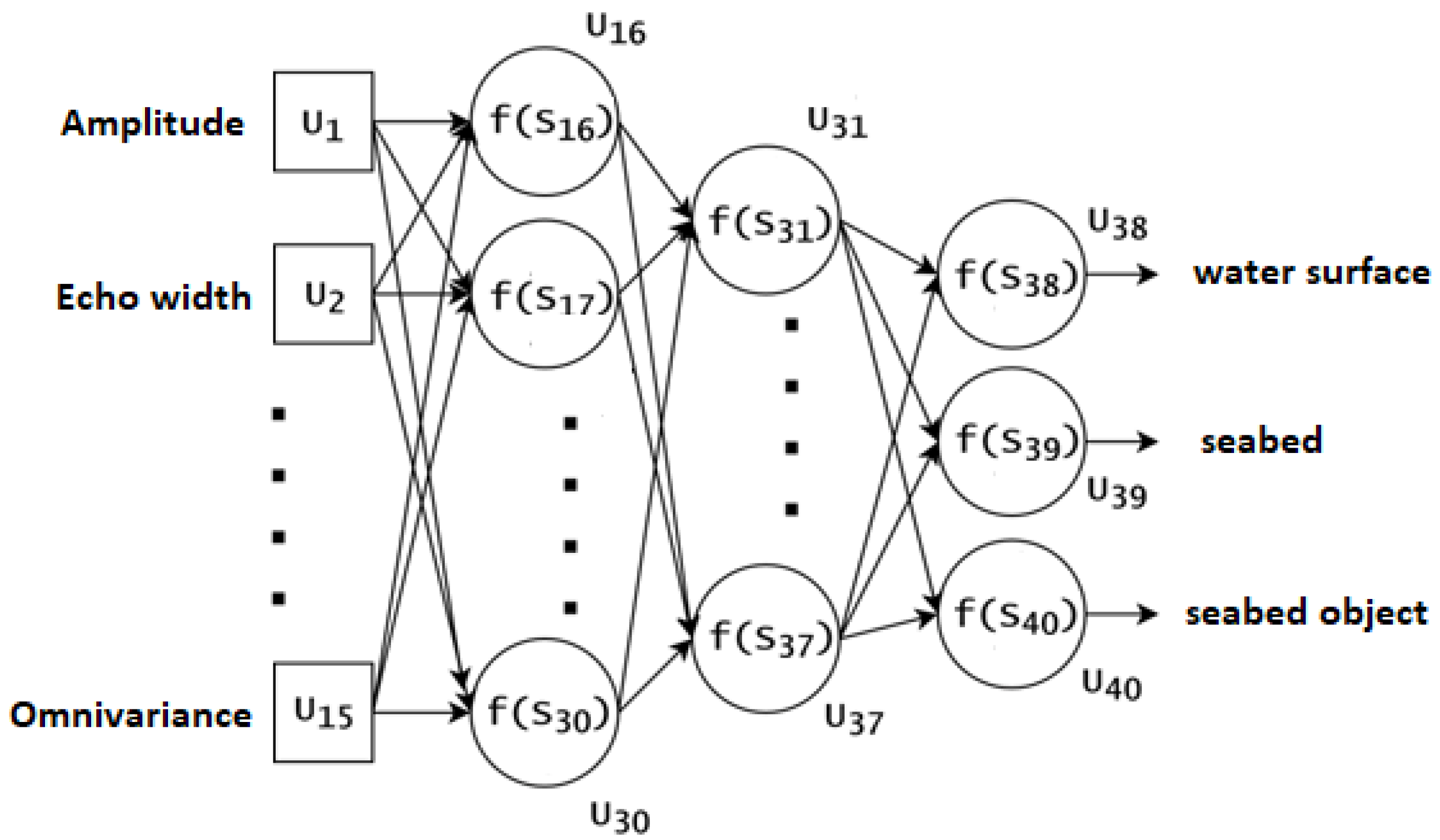
The paper is organized as follows: Section 2 describes the test area and ALB data with features and architecture of ANN. Section 3 presents the results obtained with the proposed approach and a discussion. Finally, Section 4 presents our conclusions.

2. Materials and Methods

2.1. Test Area

The test area is the artificial reef Rosenort on the Baltic Sea. It is located between Markgrafenheide and Graal-Müritz (Germany), approximately 2000 m from the coast, at a water depth of 6 m. The reef is a protected fishery reserve, and thus activities such as angling, fishing, and anchoring are prohibited. The Rosenort reef is divided into four artificially constructed zones. The zones were built from (1) 52-ton concrete tetrapods, (2) 180-ton natural stones, (3) 30 cut reef cones, and (4) six 6-ton concrete tetrapods (Figure 1).

2.2. Point Cloud and Features

The point cloud was collected in September 2013 using an AHAB Chiroptera I scanner, at a flight altitude of 400 m. The Chiroptera I scanner is equipped with two beams and scans in an elliptical shape at an angle of 20° between the scan direction and the nadir. This laser scanner uses a near-infrared (NIR) laser with a wavelength of 1064 nm at a peak measurement frequency of 400 kHz for detecting water surfaces and a green laser with a wavelength of 532 nm at a frequency of 36 kHz for underwater measurements. The horizontal nominal accuracy of the infrared beam and the green beam is 0.2 and 0.75 m, respectively, while the depth of nominal accuracy is 0.15 m. The Secchi depth achieved with the scanner exceeded 1.5 m, and during the measurement, the depth was measured at around 6.3 m. In this study, the point cloud obtained from the green beam (Figure 2) was used for analysis. The density of the point cloud obtained for the test area was 2.6 points on the water surface and 3.3 points on the underwater point (seabed and seabed object).

Scanning with the use of the AHAB Chiroptera I scanner allowed collecting the cloud of spatially coordinated points with their intensities. The analysis of such data, especially the full waveform, can provide additional information on the measured points that can aid in the classification of the acquired data. Five features (U₁–U₅,

Table 1. Description of features used to train the ANN.

Ui	Description	Formula
U1	Amplitude—the maximal peak of the Gaussian curve and is closely associated with the reflectance intensity [13]
U2	Echo width—(ω, full width at half maximum)—the width of a Gaussian curve measured between those points on the y-axis which are half the maximal peak, and in the Gaussian function, it is related to standard deviation σ	$w=2\sqrt{2 ln\left(2\right)} s$	(1)
U3	Return number (N)
U4	Number of returns (Nt)
U5	Normalized echo	$N_z=\frac{N}{N_t}$	(2)
U6	Height difference (dz)— the vertical distance between the examined point zi and the lowest zmin in the cylinder	$dz=z_i-z_{min}$	(3)
U7	Height variance $\left({\sigma }^2\right)$—a measure of dispersion and is defined as the arithmetic mean of the squares of deviations of individual values $z_i$ in the cylinder from the mean value $\overline{z}$	${\sigma }^2=\frac{1}{n}{\displaystyle \sum }_{i=1}^n{\left(z_i-\overline{z}\right)}^2$	(4)
U8	Eigenvalue λ1
U9	Eigenvalue λ2
U10	Eigenvalue λ3
U11	Sphericity—a property that describes the convexity or concavity of the analyzed point relative to points inside the cylinder	$S_{\lambda }=\frac{{\lambda }_3}{{\lambda }_1}$	(5)
U12	Planarity—a characteristic that represents the planar aspect of a point arrangement	$P_{\lambda }=\frac{{\lambda }_2-{\lambda }_3}{{\lambda }_1}$	(6)
U13	Linearity—a characteristic indicating that the distribution of points is linear (continuous).	$L_{\lambda }=\frac{{\lambda }_1-{\lambda }_2}{{\lambda }_1}$	(7)
U14	Eigentropy—defined as entropy computed from eigenvalues	$E_{\lambda }=-{\displaystyle \sum }_{i=1}^3{\lambda }_{i}ln{\lambda }_i$	(8)
U15	Omnivariance—a property whose low values are associated with flat terrain or linear structures, while high values are associated with point spatial dispersion [14]	$O_{\lambda }=\sqrt[3]{{\displaystyle \prod }_{i=1}^3{\lambda }_i}$	(9)

) derived from the full waveform, were used. A well-defined region delineated by a cylinder of a given radius r, which was 5 m (Figure 3), was used to analyze the location of each point along with its neighborhood. Features U₆–U₁₅, which describe the geometry of the point cloud, were used in the investigation.

2.3. Architecture of ANN

The raw (unbalanced) ALB data set used for training the ANN consisted of 6198 vectors (Figure 3, data in the black box). Each vector had 18 items describing the values of 15 input attributes (U1–U15, Table 1) and that of three output classes (U38–U40,

Table 2. Description of outputs from the ANN.

Ui	Description
U38	Class 1: “water surface”
U39	Class 2: “seabed”
U40	Class 3: “seabed object”

). For the error back-propagation method, 80% of these vectors were utilized for training and 20% for validating the ANN.

The three classes were labeled as follows: class 1 (U₃₈)-water surface with 2729 vectors, class 2 (U₃₉)-seabed represented by 3396 vectors, and class 3 (U₄₀)-seabed object containing 73 vectors. Since the classes had a different number of vectors, for training the ANN, the number of vectors in each class was balanced by applying different oversampling algorithms (Table 3, first column). The data set thus prepared, consisted of a different number of vectors (Table 3, last three columns), depending on the algorithm used. Imbalancing of data typically refers to classification tasks where the classes are not equally represented. Several approaches have been proposed for this issue. Among them, SMOTE has been widely used to produce synthetic samples between minority samples in the feature space. This technique improves class imbalance by linear interpolation between the underrepresented class samples [7]. It creates new instances of minority group data, by copying existing data and making minor changes. Moreover, SMOTE is a great tool for amplifying the already existing signal in minority groups without creating new signals for these groups. In general, synthetic samples are generated as a difference between the feature vector (sample) and its randomly chosen nearest neighbor. This difference is multiplied by a random number between 0 and 1 and added to the feature vector considered for creating a new sample —the synthetic one. Several improvements have been proposed for synthetic sample creation algorithms since the introduction of SMOTE. The present work included 53 oversampling methods, and a comparison of their results is provided in this paper. The data were standardized in a later step of data processing.

The ANN used in the experiments is presented in Figure 4. It is an MLP neural network [15], which has 15 inputs (U₁–U₁₅), three layers of neurons, and three outputs (U₃₈–U₄₀). The first layer comprises 15 neurons (U₁₆–U₃₀), the second layer has seven neurons (U₃₁–U₃₇), and the third layer has three neurons (U₃₈–U₄₀). Neurons in the previous layer are fully connected with those in the next layer (Figure 4). In the first layer, as well as the second layer from the bottom, all neurons possess a unipolar sigmoidal activation function, while in the last layer, all neurons (U₃₈–U₄₀) possess the soft-max activation function.

The values of the neural network outputs (U₃₈–U₄₀) inform the probability value, which indicates the degree of belonging of a given input vector to each of the three classes (water, seabed, seabed object). The ANN presented in Figure 4 was trained using an error-back propagation algorithm with the learning coefficient ro = 0.01. The maximal number of iterations was 1750.

3. Results and Discussion

The proposed approach was tested for each oversampling method by training the MLP neural network. A random starting point was used in error back-propagation. Consequently, the training procedure was repeated 11 times to obtain reliable results. After completion of each iteration, the data were tested with the dataset, which initially contained 10,612 water surface points, 13,318 seabed points, and 212 seabed object points. The results of the tests are presented in Table 3. The first two columns in the table present the names of oversampling algorithms and the year they were introduced. The next four columns show the best, worst, mean and median values of overall classification accuracy. The last four columns present the number of vectors used for training the MLP neural network.

The overall classification accuracy (Ac [%]) was calculated using the following formula:

$$Ac=\frac{\left(\frac{co{r}_w}{al{l}_w}+\frac{co{r}_s}{al{l}_s}+\frac{co{r}_o}{al{l}_o}\right)\times 100\%}{3}$$

(10)

where cor_w is the number of input vectors successfully identified as “water surface” in class 1, cor_s is the number of input vectors successfully identified as “seabed” in class 2, cor_o is the number of input vectors successfully identified as “seabed object” in class 3, and all_{w,s,o} is the total number of vectors in classes 1–3.

The best overall classification accuracy of 97.0% was achieved for the LVQ SMOTE (Learning Vector Quantization based SMOTE) algorithm. The oversampling method generated synthetic samples using codebooks obtained by learning vector quantization [16]. The second algorithm with about 96% overall classification accuracy was ROSE (Random OverSampling Examples). This algorithm works based on smoothed bootstrap resampling from data [17]. The next algorithm with the best results was PDFOS (Probability Density Function Over-Sampling), and its overall classification accuracy was about 95.8%. This algorithm generated synthetic instances as additional training data based on the estimated probability density function [18].

Table 3. Results of classification with balanced learning.

	Name	Year	Best	Worst	Mean	Median	All Vectors	Class 1	Class 2	Class 3
1	SMOTE [7]	2002	93.4	91.5	92.7	92.9	10,188	3396	3396	3396
2	SMOTE + Tomek [19]	2004	93.0	91.9	92.6	92.6	10,135	3396	3396	3343
3	SMOTE + ENN [19]	2004	93.5	90.6	92.2	92.1	9990	3396	3396	3198
4	Borderline-SMOTE1 [20]	2005	93.3	91.5	92.2	92.1	9191	2729	3396	3066
5	Borderline-SMOTE2 [20]	2005	95.4	93.4	94.7	94.8	9191	2729	3396	3066
6	SMOTE + LLE [21]	2006	91.1	88.2	89.7	89.7	10,188	3396	3396	3396
7	Distance-SMOTE [22]	2007	93.5	91.9	92.5	92.5	10,188	3396	3396	3396
8	Polynomial-SMOTE [23]	2008	91.0	88.7	90.3	90.4	13,234	5458	3396	4380
9	ADOMS [24]	2008	94.2	91.4	93.3	93.5	10,188	3396	3396	3396
10	Safe Level SMOTE [25]	2009	66.7	66.7	66.7	66.7	6573	2729	3396	448
11	MSMOTE [26]	2009	94.1	92.0	92.9	92.9	10,188	3396	3396	3396
12	SMOBD [27]	2011	95.0	92.7	93.3	93.0	10,188	3396	3396	3396
13	SVM balance [28]	2012	94.2	91.9	92.7	92.5	10,172	3396	3396	3380
14	TRIM SMOTE [29]	2012	92.4	91.5	92.0	92.0	10,188	3396	3396	3396
15	SMOTE RSB [30]	2012	81.7	66.7	71.4	67.6	7716	3396	3396	924
16	ProWSyn [31]	2013	93.6	90.6	92.4	92.5	10,188	3396	3396	3396
17	SL graph SMOTE [32]	2013	92.1	91.1	91.6	91.6	9191	2729	3396	3066
18	NRSBoundary SMOTE [33]	2013	92.6	91.4	91.8	91.8	9191	2729	3396	3066
19	LVQ SMOTE [16]	2013	97.0	94.7	96.3	96.7	10,188	3396	3396	3396
20	ROSE [17]	2014	96.0	92.5	94.6	95.0	10,188	3396	3396	3396
21	SMOTE OUT [34]	2014	93.5	91.2	92.2	92.1	10,188	3396	3396	3396
22	SMOTE Cosine [34]	2014	93.2	89.6	91.2	90.9	10,188	3396	3396	3396
23	Selected SMOTE [34]	2014	94.9	92.7	93.6	93.6	10,188	3396	3396	3396
24	LN SMOTE [35]	2011	94.4	66.7	86.3	93.5	9282	3396	3396	2490
25	MWMOTE [36]	2014	91.5	90.4	91.0	91.0	10,188	3396	3396	3396
26	PDFOS [18]	2014	95.8	92.9	94.6	94.7	10,188	3396	3396	3396
27	RWO sampling [37]	2014	93.0	88.6	91.0	91.5	10,188	3396	3396	3396
28	NEATER [38]	2014	88.0	75.8	84.8	86.5	8728	3396	3396	1936
29	DEAGO [39]	2015	85.8	85.8	85.8	85.8	10,188	3396	3396	3396
30	MCT [40]	2015	95.4	93.5	94.5	94.5	10,188	3396	3396	3396
31	SMOTE IPF [41]	2015	94.1	92.5	93.2	93.4	10,188	3396	3396	3396
32	OUPS [42]	2016	93.1	91.4	92.0	92.0	9493	3396	3396	2701
33	SMOTE D [43]	2016	81.4	78.7	80.1	80.1	10,189	3398	3396	3395
34	CE SMOTE [44]	2010	94.8	66.7	86.2	90.1	8647	2729	3396	2522
35	Edge Det SMOTE [45]	2010	93.8	92.6	93.2	93.5	10,188	3396	3396	3396
36	ASMOBD [46]	2012	88.2	86.8	87.4	87.3	10,188	3396	3396	3396
37	Assembled SMOTE [47]	2013	93.0	90.9	91.6	91.5	9191	2729	3396	3066
38	SDSMOTE [48]	2014	94.4	92.0	93.4	93.5	10,188	3396	3396	3396
39	G SMOTE [49]	2014	94.4	92.5	93.2	93.2	10,188	3396	3396	3396
40	NT SMOTE [50]	2014	93.7	92.8	93.1	93.1	10,188	3396	3396	3396
41	Lee [51]	2015	93.8	92.9	93.3	93.3	10,188	3396	3396	3396
42	MDO [52]	2016	92.1	90.3	91.3	91.4	10,188	3396	3396	3396
43	Random SMOTE [53]	2011	94.4	92.5	93.3	93.2	10,188	3396	3396	3396
44	VIS RST [54]	2016	66.7	66.6	66.7	66.7	7119	3396	3396	327
45	AND SMOTE [55]	2016	92.0	90.4	91.1	91.0	10,188	3396	3396	3396
46	NRAS [56]	2017	90.2	88.5	89.1	89.0	10,188	3396	3396	3396
47	NDO sampling [57]	2011	95.1	93.6	94.5	94.6	10,189	3397	3396	3396
48	Gaussian SMOTE [58]	2017	92.2	90.3	91.1	91.0	10,188	3396	3396	3396
49	Kmeans SMOTE [59]	2018	92.1	90.8	91.5	91.6	10,188	3396	3396	3396
50	Supervised SMOTE [60]	2014	92.8	91.5	92.1	92.1	10,188	3396	3396	3396
51	SN SMOTE [61]	2012	95.2	92.3	93.7	93.7	10,188	3396	3396	3396
52	CCR [62]	2017	88.9	87.1	88.0	88.2	9191	2729	3396	3066
53	ANS [63]	2017	91.3	88.7	90.0	90.1	9191	2729	3396	3066

Table 3. Results of classification with balanced learning.

	Name	Year	Best	Worst	Mean	Median	All Vectors	Class 1	Class 2	Class 3
1	SMOTE [7]	2002	93.4	91.5	92.7	92.9	10,188	3396	3396	3396
2	SMOTE + Tomek [19]	2004	93.0	91.9	92.6	92.6	10,135	3396	3396	3343
3	SMOTE + ENN [19]	2004	93.5	90.6	92.2	92.1	9990	3396	3396	3198
4	Borderline-SMOTE1 [20]	2005	93.3	91.5	92.2	92.1	9191	2729	3396	3066
5	Borderline-SMOTE2 [20]	2005	95.4	93.4	94.7	94.8	9191	2729	3396	3066
6	SMOTE + LLE [21]	2006	91.1	88.2	89.7	89.7	10,188	3396	3396	3396
7	Distance-SMOTE [22]	2007	93.5	91.9	92.5	92.5	10,188	3396	3396	3396
8	Polynomial-SMOTE [23]	2008	91.0	88.7	90.3	90.4	13,234	5458	3396	4380
9	ADOMS [24]	2008	94.2	91.4	93.3	93.5	10,188	3396	3396	3396
10	Safe Level SMOTE [25]	2009	66.7	66.7	66.7	66.7	6573	2729	3396	448
11	MSMOTE [26]	2009	94.1	92.0	92.9	92.9	10,188	3396	3396	3396
12	SMOBD [27]	2011	95.0	92.7	93.3	93.0	10,188	3396	3396	3396
13	SVM balance [28]	2012	94.2	91.9	92.7	92.5	10,172	3396	3396	3380
14	TRIM SMOTE [29]	2012	92.4	91.5	92.0	92.0	10,188	3396	3396	3396
15	SMOTE RSB [30]	2012	81.7	66.7	71.4	67.6	7716	3396	3396	924
16	ProWSyn [31]	2013	93.6	90.6	92.4	92.5	10,188	3396	3396	3396
17	SL graph SMOTE [32]	2013	92.1	91.1	91.6	91.6	9191	2729	3396	3066
18	NRSBoundary SMOTE [33]	2013	92.6	91.4	91.8	91.8	9191	2729	3396	3066
19	LVQ SMOTE [16]	2013	97.0	94.7	96.3	96.7	10,188	3396	3396	3396
20	ROSE [17]	2014	96.0	92.5	94.6	95.0	10,188	3396	3396	3396
21	SMOTE OUT [34]	2014	93.5	91.2	92.2	92.1	10,188	3396	3396	3396
22	SMOTE Cosine [34]	2014	93.2	89.6	91.2	90.9	10,188	3396	3396	3396
23	Selected SMOTE [34]	2014	94.9	92.7	93.6	93.6	10,188	3396	3396	3396
24	LN SMOTE [35]	2011	94.4	66.7	86.3	93.5	9282	3396	3396	2490
25	MWMOTE [36]	2014	91.5	90.4	91.0	91.0	10,188	3396	3396	3396
26	PDFOS [18]	2014	95.8	92.9	94.6	94.7	10,188	3396	3396	3396
27	RWO sampling [37]	2014	93.0	88.6	91.0	91.5	10,188	3396	3396	3396
28	NEATER [38]	2014	88.0	75.8	84.8	86.5	8728	3396	3396	1936
29	DEAGO [39]	2015	85.8	85.8	85.8	85.8	10,188	3396	3396	3396
30	MCT [40]	2015	95.4	93.5	94.5	94.5	10,188	3396	3396	3396
31	SMOTE IPF [41]	2015	94.1	92.5	93.2	93.4	10,188	3396	3396	3396
32	OUPS [42]	2016	93.1	91.4	92.0	92.0	9493	3396	3396	2701
33	SMOTE D [43]	2016	81.4	78.7	80.1	80.1	10,189	3398	3396	3395
34	CE SMOTE [44]	2010	94.8	66.7	86.2	90.1	8647	2729	3396	2522
35	Edge Det SMOTE [45]	2010	93.8	92.6	93.2	93.5	10,188	3396	3396	3396
36	ASMOBD [46]	2012	88.2	86.8	87.4	87.3	10,188	3396	3396	3396
37	Assembled SMOTE [47]	2013	93.0	90.9	91.6	91.5	9191	2729	3396	3066
38	SDSMOTE [48]	2014	94.4	92.0	93.4	93.5	10,188	3396	3396	3396
39	G SMOTE [49]	2014	94.4	92.5	93.2	93.2	10,188	3396	3396	3396
40	NT SMOTE [50]	2014	93.7	92.8	93.1	93.1	10,188	3396	3396	3396
41	Lee [51]	2015	93.8	92.9	93.3	93.3	10,188	3396	3396	3396
42	MDO [52]	2016	92.1	90.3	91.3	91.4	10,188	3396	3396	3396
43	Random SMOTE [53]	2011	94.4	92.5	93.3	93.2	10,188	3396	3396	3396
44	VIS RST [54]	2016	66.7	66.6	66.7	66.7	7119	3396	3396	327
45	AND SMOTE [55]	2016	92.0	90.4	91.1	91.0	10,188	3396	3396	3396
46	NRAS [56]	2017	90.2	88.5	89.1	89.0	10,188	3396	3396	3396
47	NDO sampling [57]	2011	95.1	93.6	94.5	94.6	10,189	3397	3396	3396
48	Gaussian SMOTE [58]	2017	92.2	90.3	91.1	91.0	10,188	3396	3396	3396
49	Kmeans SMOTE [59]	2018	92.1	90.8	91.5	91.6	10,188	3396	3396	3396
50	Supervised SMOTE [60]	2014	92.8	91.5	92.1	92.1	10,188	3396	3396	3396
51	SN SMOTE [61]	2012	95.2	92.3	93.7	93.7	10,188	3396	3396	3396
52	CCR [62]	2017	88.9	87.1	88.0	88.2	9191	2729	3396	3066
53	ANS [63]	2017	91.3	88.7	90.0	90.1	9191	2729	3396	3066

The correctly classified points constituting the seabed object were presented in the 10 confusion matrices formed for:

• unbalanced data and data with downsampling (

  Table 4. Confusion matrix of unbalanced data and data with downsampling.

  Class	Water Surface		Seabed		Seabed Object
  	(Points)	(%)	(Points)	(%)	(Points)	(%)
  Unbalance
  Water surface	10,612	100	0	0	0	0
  Seabed	0	0	13,057	98.0	261	2.0
  Seabed object	0	0	62	29.2	150	70.8
  Downsampling [64]
  Water surface	10,612	100	0	0	0	0
  Seabed	0	0	13,119	98.5	199	1.5
  Seabed object	0	0	38	17.9	174	82.1

  ) for comparison [64],
• four matrices for algorithms with the highest overall classification accuracy (

  Table 5. Confusion matrix of the four algorithms with best object detection.

  Class	Water Surface		Seabed		Seabed Object
  	(Points)	(%)	(Points)	(%)	(Points)	(%)
  LVQ SMOTE
  Water surface	10,612	100	0	0	0	0
  Seabed	0	0	12,986	97.5	332	2.5
  Seabed object	0	0	14	6.6	198	93.4
  ROSE
  Water surface	10,612	100	0	0	0	0
  Seabed	0	0	13,149	98.7	169	1.3
  Seabed object	0	0	23	10.8	189	89.2
  PDFOS
  Water surface	10,612	100	0	0	0	0
  Seabed	1	0.0	13,143	98.7	174	1.3
  Seabed object	0	0	24	11.3	188	88.7
  Borderline-SMOTE2
  Water surface	10,612	100	0	0	0	0
  Seabed	6	0.05	13,104	98.4	208	1.6
  Seabed object	0	0	26	12.3	186	87.7

  ), and
• four matrices for algorithms with the highest median overall classification accuracy in 11 repetitions (

  Table 6. Confusion matrix for the algorithms with the highest median.

  Class	Water Surface		Seabed		Seabed Object
  	(Points)	(%)	(Points)	(%)	(Points)	(%)
  LVQ SMOTE
  Water surface	10,612	100	0	0	0	0
  Seabed	0	0	13,003	97.6	315	2.4
  Seabed object	0	0	16	7.5	196	92.5
  ROSE
  Water surface	10,612	100	0	0	0	0
  Seabed	0	0	13,160	98.8	158	1.2
  Seabed object	0	0	29	13.7	183	86.3
  Borderline-SMOTE2
  Water surface	10,612	100	0	0	0	0
  Seabed	3	0.02	13,175	98.9	140	1.1
  Seabed object	0	0	31	14.6	181	85.4
  PDFOS
  Water surface	10,612	100	0	0	0	0
  Seabed	1	0.01	13,212	99.2	105	0.8
  Seabed object	0	0	32	15.1	180	84.9

  ).

The overall classification accuracy achieved for unbalanced data was 89.6% and for downsampling data was 93.5% [64]. The downsampling method was used, in which each class was given the same number of vectors, similar to in class 3. The data set, divided into three equal classes, contained a total of 219 input vectors (3 × 79). Downsampling contributed to increasing the overall classification accuracy by 3.9%. The correct classification of points in class 3 also increased by 11.3%.

Table 5 and Table 6 present the confusion matrix for the four algorithms with the best object detection results and four algorithms with the best median values. The correct classification of points in class 3 (seabed object) ranged between 89.7% and 93.4% for the best results of imbalanced learning and between 84.9% and 92.5% for median results. In all cases, an increase in the overall classification accuracy and point detection on the seabed objects was achieved. The water surface was classified with an accuracy of 100% in all algorithms. Two algorithms—Safe Level SMOTE and VIS RST—were found to be ineffective and as a result, none of the points on the objects were detected.

The accuracy of oversampling algorithms was assessed using three accuracy evaluation indices: precision, recall, and F1-score.

Precision refers to the proportion of correctly predicted points on the object to all points on the object, i.e.,

$$\mathrm{Precision}=\frac{TP}{TP+FP}$$

(11)

Recall: refers to the proportion of the correctly predicted points on the object to all points on the object, i.e.,

$$\mathrm{Recall}=\frac{TP}{TP+FN}$$

(12)

F1-score refers to the harmonic mean of precision and recall, i.e.,

$$\mathrm{F}1-\mathrm{score}=\frac{2TP}{2TP+FP+FN}$$

(13)

where TP, TN, FP, and FN denote true positive, true negative, false positive, and false negative, respectively.

The indices were computed for the median of results. Recall was found to be high for all four algorithms: 0.92 for LVQ SMOTE, 0.86 for ROSE, 0.85 for borderline-SMOTE2, and 0.84 for PDFOS. The F1-score for class 3 was calculated to be 0.54, 0.66, 0.68, and 0.72, respectively. Among the oversampling algorithms, MDO had the best F1-score of 0.75, which was comparable with that of PDFOS. The overall accuracy of the median results of MDO was 91.4, and the confusion matrix of the median results is presented in

Table 7. Confusion matrix of median results for algorithm MDO.

Class	Water Surface		Seabed		Seabed Object
	(Points)	(%)	(Points)	(%)	(Points)	(%)
MDO
Water surface	10,612	100	0	0	0	0
Seabed	0	0	13,266	99.6	52	0.4
Seabed object	0	0	54	25.5	158	74.5

.

4. Conclusions

ALB technique follows existing water reservoir measurement patterns. Monitoring the seabed and detection of seabed objects in the coastal zone around ports with heavy vessel traffic help in decreasing the risk of maritime grounding and collision with underwater obstacles, thereby reducing the probability of environmental incidents that can occur due to cargo and fuel leakage or even unexploded ordnance explosion.

This study used a total of 53 oversampling algorithms with imbalanced MLP neural learning for the classification of the ALB data and detection of seabed objects. The results revealed that selected oversampling algorithms classified point clouds better than unbalanced data or data with simple downsampling. The algorithms that produced the best results can be divided into two groups: (1) the algorithms with good recall, which improves the detection of points on objects—LVQ SMOTE and ROSE; and (2) those that improve the general classification with the highest F1-score—MDO and PDFOS. Identifying the oversampling method that gives the best results for object classification and detection is challenging. This is because a good recall is often associated with false classification of points.

As the present study did not cover all the issues related to the subject, future work should focus on using SMOTE methods for improving the detection of underwater objects. Additionally, the possibility of applying SMOTE in deep-sea bottom imaging using MBES would be a topic of interest.

References

1. Muirhead, K.; Cracknell, A.P. Airborne Lidar Bathymetry. Int. J. Remote Sens. 1986, 7, 597–614. [Google Scholar] [CrossRef]
2. Wang, C.-K.; Philpot, W.D. Using Airborne Bathymetric Lidar to Detect Bottom Type Variation in Shallow Waters. Remote Sens. Environ. 2007, 106, 123–135. [Google Scholar] [CrossRef]
3. Yeu, Y.; Yee, J.-J.; Yun, H.S.; Kim, K.B. Evaluation of the Accuracy of Bathymetry on the Nearshore Coastlines of Western Korea from Satellite Altimetry, Multi-Beam, and Airborne Bathymetric LiDAR. Sensors 2018, 18, 2926. [Google Scholar] [CrossRef] [PubMed] [Green Version]
4. Stępień, G.; Tomczak, A.; Loosaar, M.; Ziębka, T. Dimensioning Method of Floating Offshore Objects by Means of Quasi-Similarity Transformation with Reduced Tolerance Errors. Sensors 2020, 20, 6497. [Google Scholar] [CrossRef]
5. Costa, B.M.; Battista, T.A.; Pittman, S.J. Comparative Evaluation of Airborne LiDAR and Ship-Based Multibeam SoNAR Bathymetry and Intensity for Mapping Coral Reef Ecosystems. Remote Sens. Environ. 2009, 113, 1082–1100. [Google Scholar] [CrossRef]
6. Jung, J.; Lee, J.; Parrish, C.E. Inverse Histogram-Based Clustering Approach to Seafloor Segmentation from Bathymetric Lidar Data. Remote Sens. 2021, 13, 3665. [Google Scholar] [CrossRef]
7. Chawla, N.V.; Bowyer, K.W.; Hall, L.O.; Kegelmeyer, W.P. SMOTE: Synthetic Minority Over-Sampling Technique. J. Artif. Intell. Res. 2002, 16, 321–357. [Google Scholar] [CrossRef]
8. Herrault, P.-A.; Poterek, Q.; Keller, B.; Schwartz, D.; Ertlen, D. Automated Detection of Former Field Systems from Airborne Laser Scanning Data: A New Approach for Historical Ecology. Int. J. Appl. Earth Obs. Geoinf. 2021, 104, 102563. [Google Scholar] [CrossRef]
9. Chasco-Hernández, D.; Sanz-Delgado, J.A.; García-Morales, V.; Álvarez-Mozos, J. Automatic Detection of High-Voltage Power Lines in LiDAR Surveys Using Data Mining Techniques. In Advances in Design Engineering; Lecture Notes in Mechanical Engineering; Cavas-Martínez, F., Sanz-Adan, F., Morer Camo, P., Lostado Lorza, R., Santamaría Peña, J., Eds.; Springer International Publishing: Cham, Switzerland, 2020; pp. 568–575. ISBN 978-3-030-41199-2. [Google Scholar]
10. Al-Najjar, H.A.H.; Pradhan, B.; Sarkar, R.; Beydoun, G.; Alamri, A. A New Integrated Approach for Landslide Data Balancing and Spatial Prediction Based on Generative Adversarial Networks (GAN). Remote Sens. 2021, 13, 4011. [Google Scholar] [CrossRef]
11. Eren, F.; Pe’eri, S.; Rzhanov, Y.; Ward, L. Bottom Characterization by Using Airborne Lidar Bathymetry (ALB) Waveform Features Obtained from Bottom Return Residual Analysis. Remote Sens. Environ. 2018, 206, 260–274. [Google Scholar] [CrossRef]
12. Aissou, B.E.; Aissa, A.B.; Dairi, A.; Harrou, F.; Wichmann, A.; Kada, M. Building Roof Superstructures Classification from Imbalanced and Low Density Airborne LiDAR Point Cloud. IEEE Sens. J. 2021, 21, 14960–14976. [Google Scholar] [CrossRef]
13. Wagner, W.; Ullrich, A.; Ducic, V.; Melzer, T.; Studnicka, N. Gaussian Decomposition and Calibration of a Novel Small-Footprint Full-Waveform Digitising Airborne Laser Scanner. ISPRS J. Photogramm. Remote Sens. 2006, 60, 100–112. [Google Scholar] [CrossRef]
14. Niemeyer, J.; Rottensteiner, F.; Soergel, U. Contextual Classification of Lidar Data and Building Object Detection in Urban Areas. ISPRS J. Photogramm. Remote Sens. 2014, 87, 152–165. [Google Scholar] [CrossRef]
15. Shibata, K.; Ikeda, Y. Effect of Number of Hidden Neurons on Learning in Large-Scale Layered Neural Networks. In Proceedings of the 2009 ICCAS-SICE, Fukuoka, Japan, 18–21 August 2009; pp. 5008–5013. [Google Scholar]
16. Nakamura, M.; Kajiwara, Y.; Otsuka, A.; Kimura, H. LVQ-SMOTE—Learning Vector Quantization Based Synthetic Minority Over–Sampling Technique for Biomedical Data. BioData Min. 2013, 6, 16. [Google Scholar] [CrossRef] [PubMed] [Green Version]
17. Menardi, G.; Torelli, N. Training and Assessing Classification Rules with Imbalanced Data. Data Min. Knowl. Disc. 2014, 28, 92–122. [Google Scholar] [CrossRef]
18. Gao, M.; Hong, X.; Chen, S.; Harris, C.J.; Khalaf, E. PDFOS: PDF Estimation Based over-Sampling for Imbalanced Two-Class Problems. Neurocomputing 2014, 138, 248–259. [Google Scholar] [CrossRef]
19. Batista, G.E.A.P.A.; Prati, R.C.; Monard, M.C. A Study of the Behavior of Several Methods for Balancing Machine Learning Training Data. SIGKDD Explor. Newsl. 2004, 6, 20–29. [Google Scholar] [CrossRef]
20. Han, H.; Wang, W.-Y.; Mao, B.-H. Borderline-SMOTE: A New Over-Sampling Method in Imbalanced Data Sets Learning. In Advances in Intelligent Computing; Huang, D.-S., Zhang, X.-P., Huang, G.-B., Eds.; Springer: Berlin/Heidelberg, Germany, 2005; pp. 878–887. [Google Scholar]
21. Wang, J.; Xu, M.; Wang, H.; Zhang, J. Classification of Imbalanced Data by Using the SMOTE Algorithm and Locally Linear Embedding. In Proceedings of the 2006 8th International Conference on Signal Processing, Beijing, China, 16–20 November 2006; Volume 3. [Google Scholar]
22. Calleja, J.L.; Fuentes, O. A Distance-Based Over-Sampling Method for Learning from Imbalanced Data Sets. In Proceedings of the FLAIRS Conference, Florida, FL, USA, 7–9 May 2007. [Google Scholar]
23. Gazzah, S.; Amara, N.E.B. New Oversampling Approaches Based on Polynomial Fitting for Imbalanced Data Sets. In Proceedings of the 2008 The Eighth IAPR International Workshop on Document Analysis Systems, Nara, Japan, 16–19 September 2008; IEEE: Piscataway, NJ, USA, 2008; pp. 677–684. [Google Scholar]
24. Tang, S.; Chen, S. The Generation Mechanism of Synthetic Minority Class Examples. In Proceedings of the 2008 International Conference on Information Technology and Applications in Biomedicine, Shenzhen, China, 30–31 May 2008; pp. 444–447. [Google Scholar]
25. Bunkhumpornpat, C.; Sinapiromsaran, K.; Lursinsap, C. Safe-Level-SMOTE: Safe-Level-Synthetic Minority Over-Sampling TEchnique for Handling the Class Imbalanced Problem. In Advances in Knowledge Discovery and Data Mining; Theeramunkong, T., Kijsirikul, B., Cercone, N., Ho, T.-B., Eds.; Springer: Berlin/Heidelberg, Germany, 2009; pp. 475–482. [Google Scholar]
26. Hu, S.; Liang, Y.; Ma, L.; He, Y. MSMOTE: Improving Classification Performance When Training Data Is Imbalanced. In Proceedings of the 2009 Second International Workshop on Computer Science and Engineering, Qingdao, China, 28 October 2009; IEEE: Piscataway, NJ, USA, 2009; pp. 13–17. [Google Scholar]
27. Cao, Q.; Wang, S. Applying Over-Sampling Technique Based on Data Density and Cost-Sensitive SVM to Imbalanced Learning. In Proceedings of the 2011 International Conference on Information Management, Innovation Management and Industrial Engineering, Shenzhen, China, 26–27 November 2011; Volume 2, pp. 543–548. [Google Scholar]
28. Farquad, M.A.H.; Bose, I. Preprocessing Unbalanced Data Using Support Vector Machine. Decis. Support Syst. 2012, 53, 226–233. [Google Scholar] [CrossRef]
29. Puntumapon, K.; Waiyamai, K. A Pruning-Based Approach for Searching Precise and Generalized Region for Synthetic Minority Over-Sampling. In Advances in Knowledge Discovery and Data Mining; Tan, P.-N., Chawla, S., Ho, C.K., Bailey, J., Eds.; Springer: Berlin/Heidelberg, Germany, 2012; pp. 371–382. [Google Scholar]
30. Ramentol, E.; Caballero, Y.; Bello, R.; Herrera, F. SMOTE-RSB*: A Hybrid Preprocessing Approach Based on Oversampling and Undersampling for High Imbalanced Data-Sets Using SMOTE and Rough Sets Theory. Knowl. Inf. Syst. 2012, 33, 245–265. [Google Scholar] [CrossRef]
31. Barua, S.; Islam, M.M.; Murase, K. ProWSyn: Proximity Weighted Synthetic Oversampling Technique for Imbalanced Data Set Learning. In Advances in Knowledge Discovery and Data Mining; Pei, J., Tseng, V.S., Cao, L., Motoda, H., Xu, G., Eds.; Springer: Berlin/Heidelberg, Germany, 2013; pp. 317–328. [Google Scholar]
32. Bunkhumpornpat, C.; Subpaiboonkit, S. Safe Level Graph for Synthetic Minority Over-Sampling Techniques. In Proceedings of the 2013 13th International Symposium on Communications and Information Technologies (ISCIT), Surat Thani, Thailand, 4–6 September 2013; pp. 570–575. [Google Scholar]
33. Hu, F.; Li, H. A Novel Boundary Oversampling Algorithm Based on Neighborhood Rough Set Model: NRSBoundary-SMOTE. Math. Probl. Eng. 2013, 2013, 694809. [Google Scholar] [CrossRef]
34. Koto, F. SMOTE-Out, SMOTE-Cosine, and Selected-SMOTE: An Enhancement Strategy to Handle Imbalance in Data Level. In Proceedings of the 2014 International Conference on Advanced Computer Science and Information System, Jakarta, Indonesia, 18–19 October 2014; IEEE: Piscataway, NJ, USA, 2014; pp. 280–284. [Google Scholar]
35. Maciejewski, T.; Stefanowski, J. Local Neighbourhood Extension of SMOTE for Mining Imbalanced Data. In Proceedings of the 2011 IEEE Symposium on Computational Intelligence and Data Mining (CIDM), Paris, France, 11–15 April 2011; IEEE: Piscataway, NJ, USA, 2011; pp. 104–111. [Google Scholar]
36. Barua, S.; Islam, M.M.; Yao, X.; Murase, K. MWMOTE–Majority Weighted Minority Oversampling Technique for Imbalanced Data Set Learning. IEEE Trans. Knowl. Data Eng. 2014, 26, 405–425. [Google Scholar] [CrossRef]
37. Zhang, H.; Li, M. RWO-Sampling: A Random Walk over-Sampling Approach to Imbalanced Data Classification. Inf. Fusion 2014, 20, 99–116. [Google Scholar] [CrossRef]
38. Almogahed, B.A.; Kakadiaris, I.A. NEATER: Filtering of over-Sampled Data Using Non-Cooperative Game Theory. Soft Comput. 2015, 19, 3301–3322. [Google Scholar] [CrossRef]
39. Bellinger, C.; Japkowicz, N.; Drummond, C. Synthetic Oversampling for Advanced Radioactive Threat Detection. In Proceedings of the 2015 IEEE 14th International Conference on Machine Learning and Applications (ICMLA), Miami, FL, USA, 9–11 December 2015; IEEE: Piscataway, NJ, USA, 2015; pp. 948–953. [Google Scholar]
40. Jiang, L.; Qiu, C.; Li, C. A Novel Minority Cloning Technique for Cost-Sensitive Learning. Int. J. Patt. Recogn. Artif. Intell. 2015, 29, 1551004. [Google Scholar] [CrossRef]
41. Sáez, J.A.; Luengo, J.; Stefanowski, J.; Herrera, F. SMOTE–IPF: Addressing the Noisy and Borderline Examples Problem in Imbalanced Classification by a Re-Sampling Method with Filtering. Inf. Sci. 2015, 291, 184–203. [Google Scholar] [CrossRef]
42. Rivera, W.A.; Xanthopoulos, P. A Priori Synthetic Over-Sampling Methods for Increasing Classification Sensitivity in Imbalanced Data Sets. Expert Syst. Appl. 2016, 66, 124–135. [Google Scholar] [CrossRef]
43. Torres, F.R.; Carrasco-Ochoa, J.A.; Martínez-Trinidad, J.F. SMOTE-D a Deterministic Version of SMOTE. In Pattern Recognition; Martínez-Trinidad, J.F., Carrasco-Ochoa, J.A., Ayala Ramirez, V., Olvera-López, J.A., Jiang, X., Eds.; Springer International Publishing: Cham, Switzerland, 2016; pp. 177–188. [Google Scholar]
44. Chen, S.; Guo, G.; Chen, L. A New Over-Sampling Method Based on Cluster Ensembles. In Proceedings of the 2010 IEEE 24th International Conference on Advanced Information Networking and Applications Workshops, Perth, Australia, 20–23 April 2010; IEEE: Piscataway, NJ, USA, 2010; pp. 599–604. [Google Scholar]
45. Kang, Y.-I.; Won, S. Weight Decision Algorithm for Oversampling Technique on Class-Imbalanced Learning. In Proceedings of the ICCAS 2010, Gyeonggi-do, Korea, 27–30 October 2010; pp. 182–186. [Google Scholar]
46. Wang, S.; Li, Z.; Chao, W.; Cao, Q. Applying Adaptive Over-Sampling Technique Based on Data Density and Cost-Sensitive SVM to Imbalanced Learning. In Proceedings of the The 2012 International Joint Conference on Neural Networks (IJCNN), Brisbane, Australia, 10–15 June 2012; pp. 1–8. [Google Scholar]
47. Zhou, B.; Yang, C.; Guo, H.; Hu, J. A Quasi-Linear SVM Combined with Assembled SMOTE for Imbalanced Data Classification. In Proceedings of the The 2013 International Joint Conference on Neural Networks (IJCNN), Dallas, TX, USA, 4–9 August 2013; pp. 1–7. [Google Scholar]
48. Li, K.; Zhang, W.; Lu, Q.; Fang, X. An Improved SMOTE Imbalanced Data Classification Method Based on Support Degree. In Proceedings of the 2014 International Conference on Identification, Information and Knowledge in the Internet of Things, Beijing, China, 17–18 October 2014; pp. 34–38. [Google Scholar]
49. Sandhan, T.; Choi, J.Y. Handling Imbalanced Datasets by Partially Guided Hybrid Sampling for Pattern Recognition. In Proceedings of the 2014 22nd International Conference on Pattern Recognition, Stockholm, Sweden, 24–28 August 2014; pp. 1449–1453. [Google Scholar]
50. Xu, Y.H.; Li, H.; Le, L.P.; Tian, X.Y. Neighborhood Triangular Synthetic Minority Over-Sampling Technique for Imbalanced Prediction on Small Samples of Chinese Tourism and Hospitality Firms. In Proceedings of the 2014 Seventh International Joint Conference on Computational Sciences and Optimization, Washington, DC, USA, 4–6 July 2014; pp. 534–538. [Google Scholar]
51. Lee, J.; Kim, N.; Lee, J.-H. An Over-Sampling Technique with Rejection for Imbalanced Class Learning. In Proceedings of the 9th International Conference on Ubiquitous Information Management and Communication, Bali, Indonesia, 8–10 January 2015; ACM: New York, NY, USA, 2015; pp. 1–6. [Google Scholar]
52. Abdi, L.; Hashemi, S. To Combat Multi-Class Imbalanced Problems by Means of Over-Sampling Techniques. IEEE Trans. Knowl. Data Eng. 2016, 28, 238–251. [Google Scholar] [CrossRef]
53. Dong, Y.; Wang, X. A New Over-Sampling Approach: Random-SMOTE for Learning from Imbalanced Data Sets. In Knowledge Science, Engineering and Management; Xiong, H., Lee, W.B., Eds.; Springer: Berlin/Heidelberg, Germany, 2011; pp. 343–352. [Google Scholar]
54. Borowska, K.; Stepaniuk, J. Imbalanced Data Classification: A Novel Re-Sampling Approach Combining Versatile Improved SMOTE and Rough Sets. In Computer Information Systems and Industrial Management; Saeed, K., Homenda, W., Eds.; Springer International Publishing: Cham, Switzerland, 2016; pp. 31–42. [Google Scholar]
55. Yun, J.; Ha, J.; Lee, J.-S. Automatic Determination of Neighborhood Size in SMOTE. In Proceedings of the 10th International Conference on Ubiquitous Information Management and Communication, Danang, Viet Nam, 4–6 January 2016; ACM: New York, NY, USA, 2015; pp. 1–8. [Google Scholar]
56. Rivera, W.A. Noise Reduction A Priori Synthetic Over-Sampling for Class Imbalanced Data Sets. Inf. Sci. 2017, 408, 146–161. [Google Scholar] [CrossRef]
57. Zhang, L.; Wang, W. A Re-Sampling Method for Class Imbalance Learning with Credit Data. In Proceedings of the 2011 International Conference of Information Technology, Computer Engineering and Management Sciences, Nanjing, China, 24–25 September 2011; Volume 1, pp. 393–397. [Google Scholar]
58. Lee, H.; Kim, J.; Kim, S. Gaussian-Based SMOTE Algorithm for Solving Skewed Class Distributions. Int. J. Fuzzy Log. Intell. Syst. 2017, 17, 229–234. [Google Scholar] [CrossRef]
59. Douzas, G.; Bacao, F.; Last, F. Improving Imbalanced Learning through a Heuristic Oversampling Method Based on K-Means and SMOTE. Inf. Sci. 2018, 465, 1–20. [Google Scholar] [CrossRef] [Green Version]
60. Hu, J.; He, X.; Yu, D.-J.; Yang, X.-B.; Yang, J.-Y.; Shen, H.-B. A New Supervised Over-Sampling Algorithm with Application to Protein-Nucleotide Binding Residue Prediction. PLoS ONE 2014, 9, e107676. [Google Scholar] [CrossRef] [PubMed]
61. García, V.; Sánchez, J.S.; Martín-Félez, R.; Mollineda, R.A. Surrounding Neighborhood-Based SMOTE for Learning from Imbalanced Data Sets. Prog Artif. Intell. 2012, 1, 347–362. [Google Scholar] [CrossRef] [Green Version]
62. Koziarski, M.; Wozniak, M. CCR: A Combined Cleaning and Resampling Algorithm for Imbalanced Data Classification. Int. J. Appl. Math. Comput. Sci. 2017, 27, 727–736. [Google Scholar] [CrossRef] [Green Version]
63. Siriseriwan, W.; Sinapiromsaran, K. Adaptive Neighbor Synthetic Minority Oversampling Technique under 1NN Outcast Handling. Songklanakarin J. Sci. Technol. 2017, 39, 565–576. [Google Scholar] [CrossRef]
64. Kogut, T.; Slowik, A. Classification of Airborne Laser Bathymetry Data Using Artificial Neural Networks. IEEE J. Sel. Top. Appl. Earth Obs. Remote Sens. 2021, 14, 1959–1966. [Google Scholar] [CrossRef]
Figure 1. Location of the test area (approximately 25 km north of the city of Rostock in Germany).
Sensors 22 03121 g001
Figure 2. Three classes in the ALB point cloud (blue—water surface, class 1; green—seabed, class 2; red—points on the object on the seabed, class 3).
Sensors 22 03121 g002
Figure 3. Visualization of the cylinder and analyzed points (red—analyzed point, green—points inside the cylinder used to compute the features, grey—other points in the point cloud, r—radius).
Sensors 22 03121 g003
Figure 4. The architecture of ANN.
Sensors 22 03121 g004