
Musical Instrument Identification Using Deep Learning Approach


Abstract
:1. Introduction
2. Study Background
2.1. Metadata
- Basic: based on the value of the audio signal samples;
- BasicSpectral: simple time–frequency signal analysis;
- SpectralBasis: one-dimensional spectral projection of a signal prepared primarily to facilitate signal classification;
- SignalParameters: information about the periodicity of the signal;
- TimbralTemporal: time and musical timbre features;
- TimbralSpectral: description of the linear–frequency relationships in the signal.
2.2. Related Work
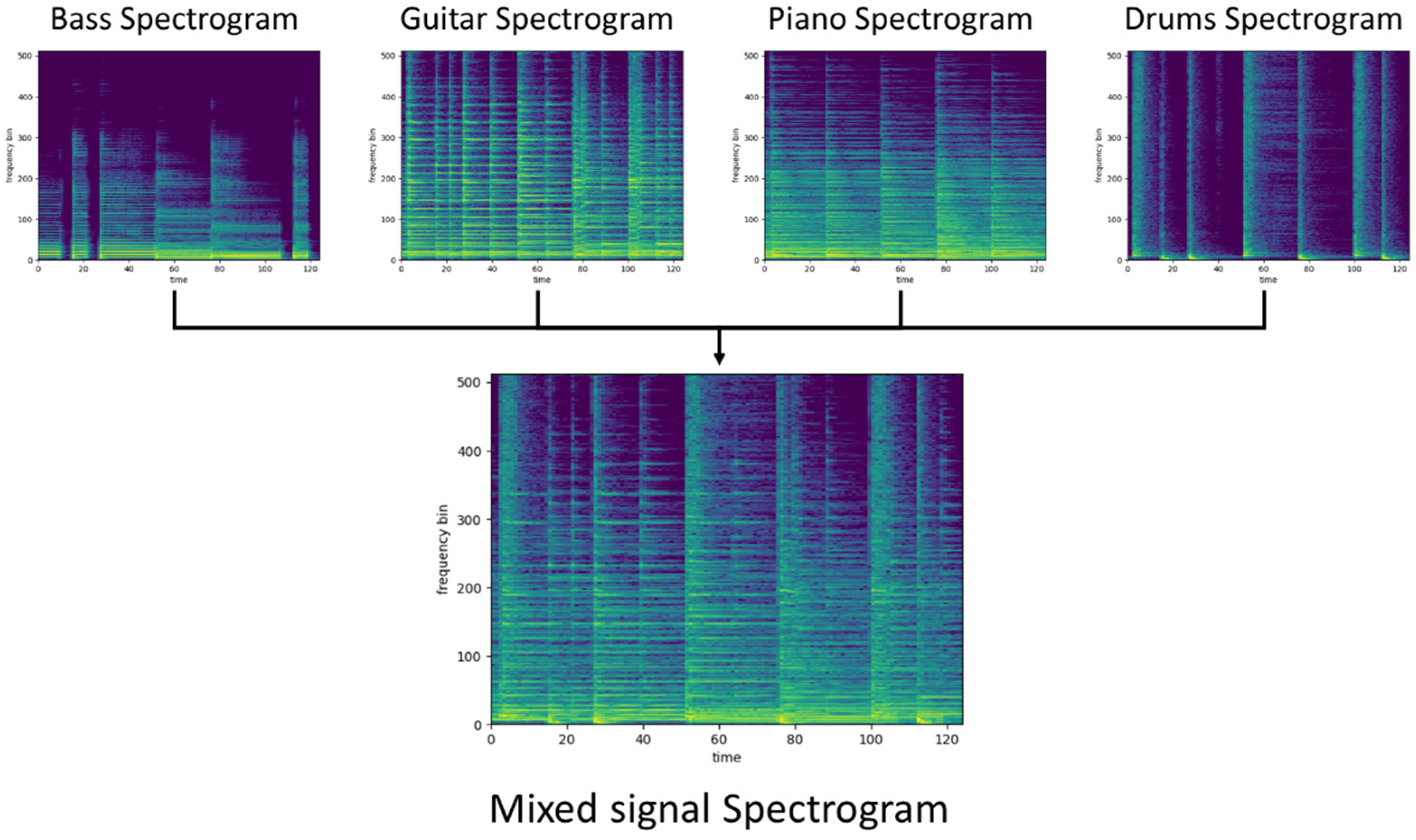
3. Dataset
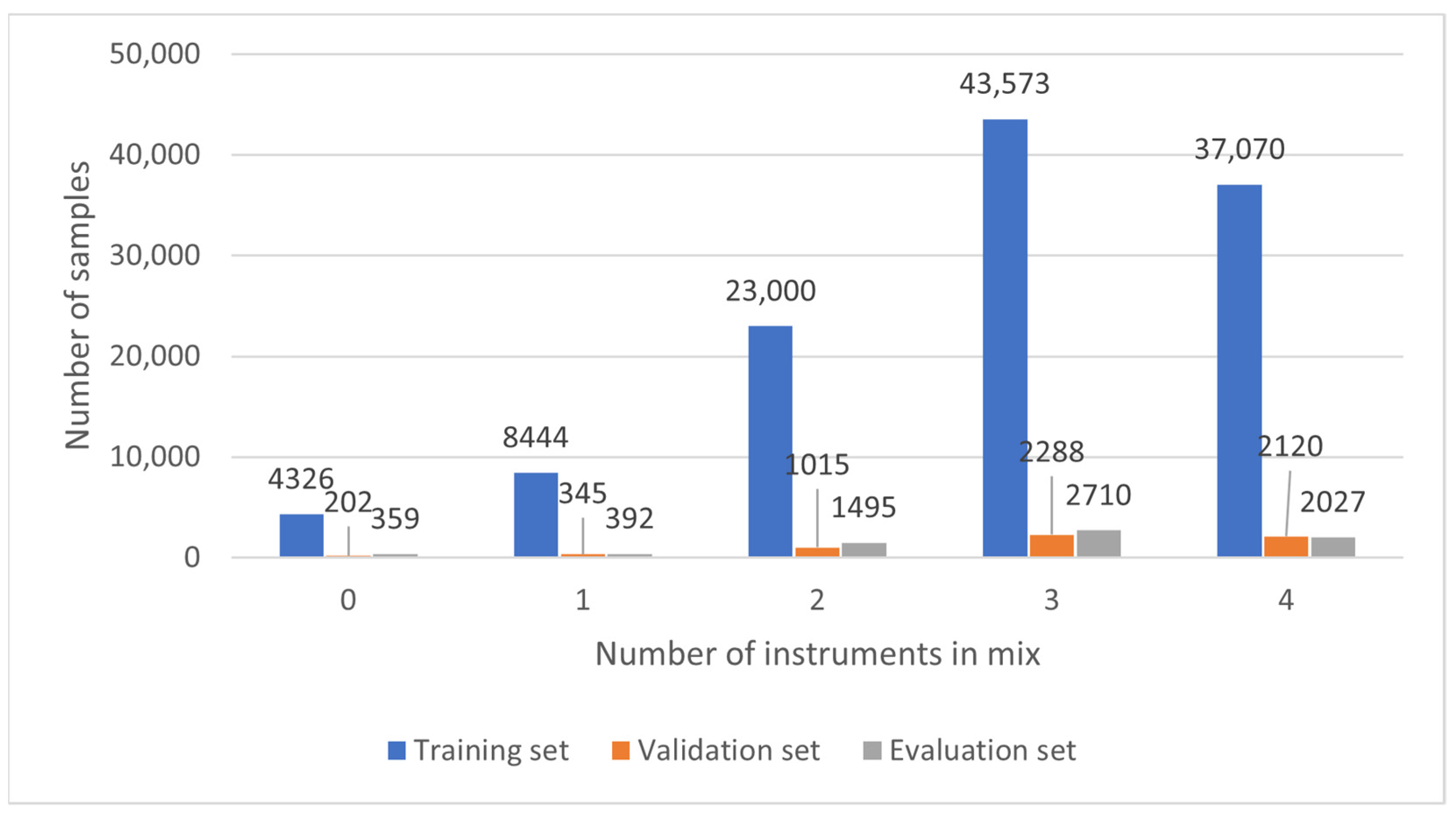
- Training set—116,413 examples;
- Validation set—5970 examples;
- Evaluation set—6983 examples.
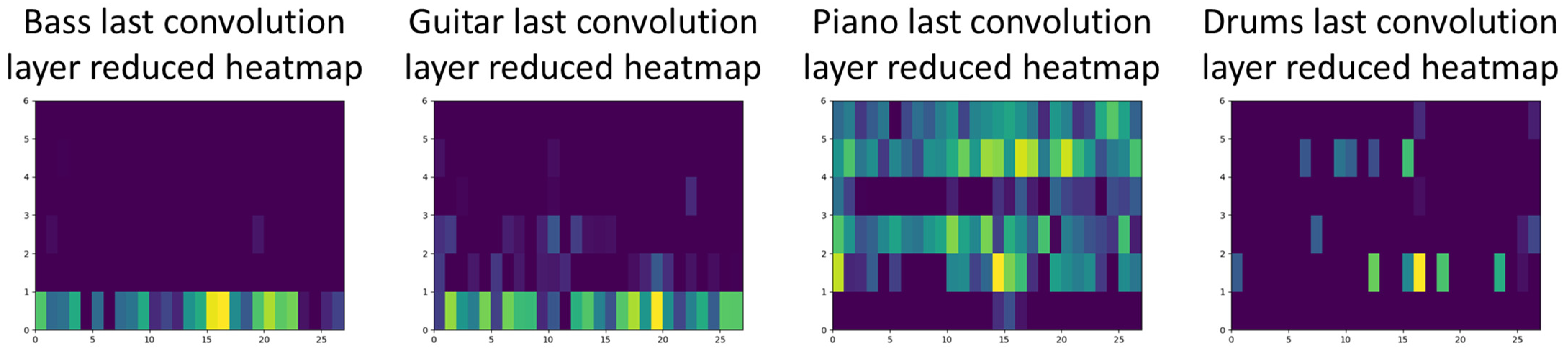
- 4.
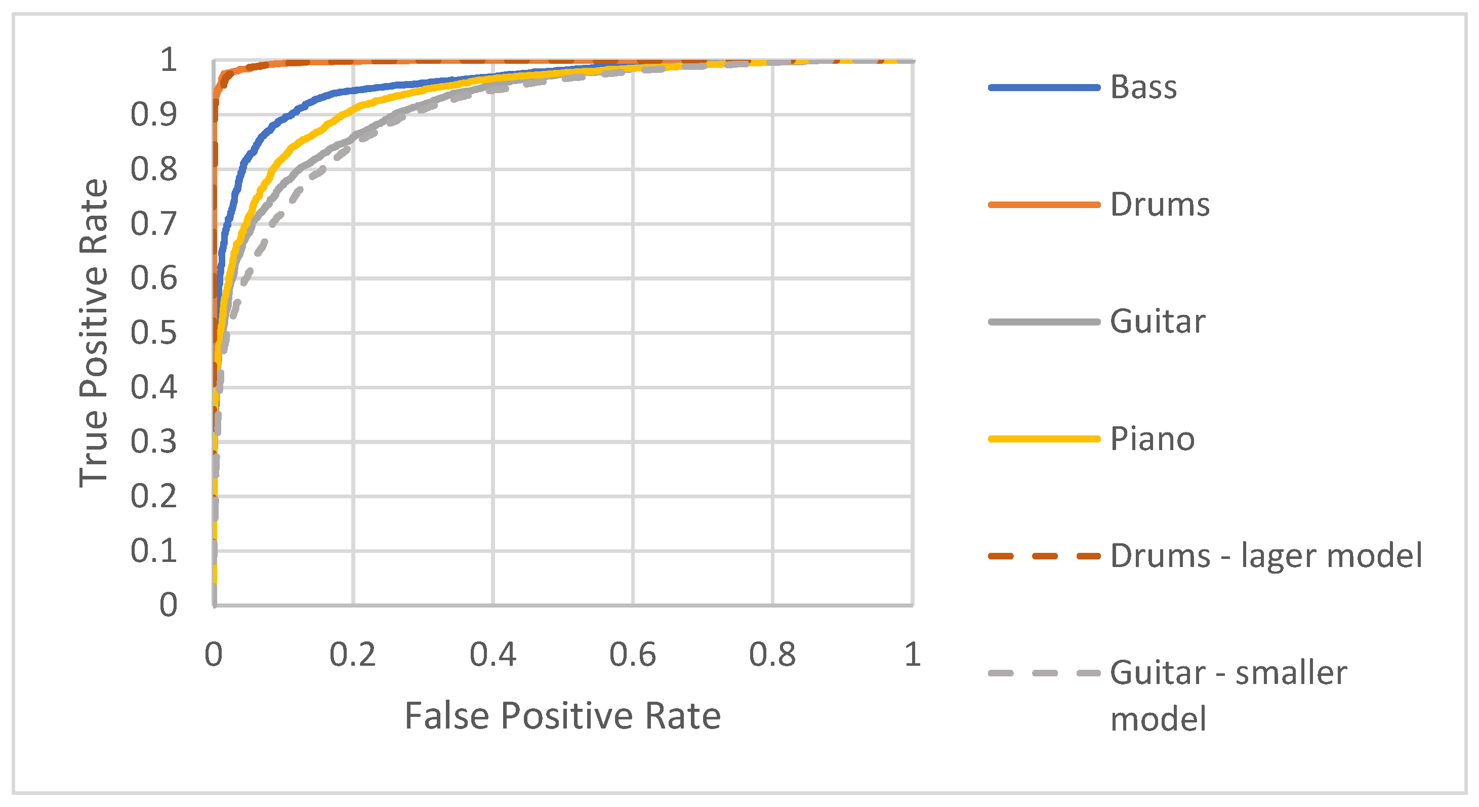
- Bass—0.65
- 5.
- Guitar—1.0
- 6.
- Piano—0.78
- 7.
- Drums—0.56
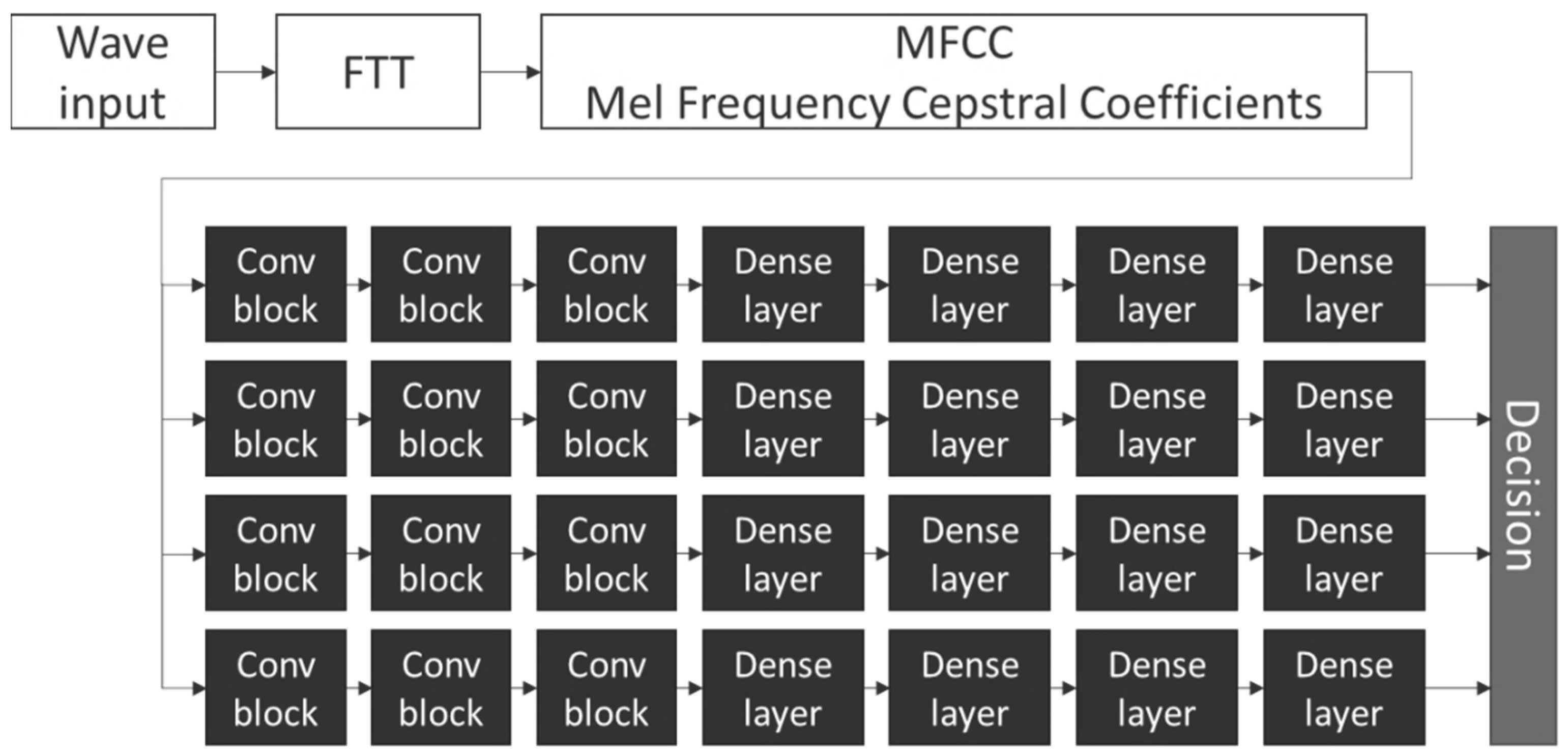
4. Model
- 1024 samples Hamming window length;
- 512 samples window step;
- 40 MFCC bins.
- dense_outputs = []
- input = Input(shape = input_shape)
- mfcc = prepareMfccModel(input)
- dense_outputs.append(prepareBassModel(mfcc))
- dense_outputs.append(prepareGuitarModel(mfcc))
- dense_outputs.append(preparePianoModel(mfcc))
- dense_outputs.append(prepareDrumsModel(mfcc))
- concat = Concatenate()(dense_outputs)
- model = Model(inputs = input, outputs = concat)
- return model
4.1. Training
4.2. Evaluation Results and Discussion
- Precision—0.92;
- Recall—0.93;
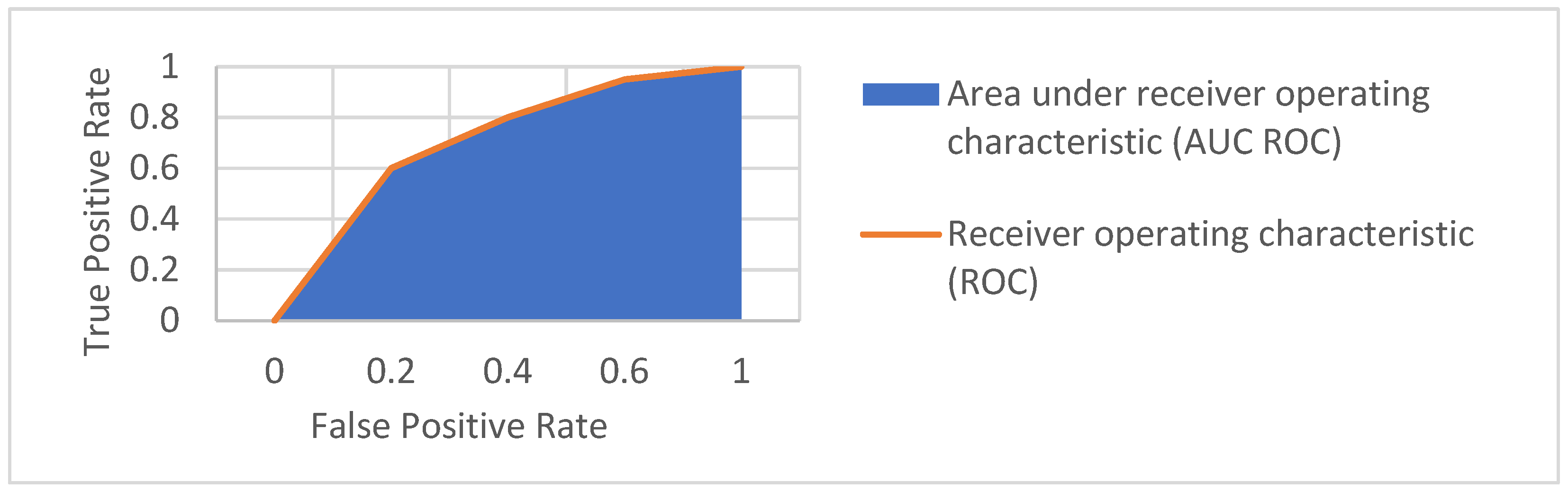
- AUC ROC—0.96;
- F1 score—0.93.
- True positive—17,759;
- True negative—6610;
- False positive—1512;
- False negative—1319.
4.3. Redefining the Models
4.4. Evaluation Result Comparison
5. Discussion
6. Conclusions
Author Contributions
Funding
Institutional Review Board Statement
Informed Consent Statement
Data Availability Statement
Conflicts of Interest
References
- Heran, C.; Bhakta, H.C.; Choday, V.K.; Grover, W.H. Musical Instruments as Sensors. ACS Omega 2018, 3, 11026–11103. [Google Scholar] [CrossRef]
- Tanaka, A. Sensor-based musical instruments and interactive music. In The Oxford Handbook of Computer Music; Dean, T.T., Ed.; Oxford University Press: Oxford, UK, 2012. [Google Scholar] [CrossRef]
- Turchet, L.; McPherson, A.; Fischione, C. Smart instruments: Towards an ecosystem of interoperable devices connecting performers and audiences. In Proceedings of the Sound and Music Computing Conference, Hamburg, Germany, 31 August–3 September 2016; pp. 498–505. [Google Scholar]
- Turchet, L.; McPherson, A.; Barthet, M. Real-Time Hit Classification in Smart Cajón. Front. ICT 2018, 5, 16. [Google Scholar] [CrossRef]
- Benetos, E.; Dixon, S.; Giannoulis, D.; Kirchhoff, H.; Klapuri, A. Automatic music transcription: Challenges and future directions. J. Intell. Inf. Syst. 2013, 41, 407–434. [Google Scholar] [CrossRef] [Green Version]
- Brown, J.C. Computer Identification of Musical Instruments using Pattern Recognition with Cepstral Coefficients as Features. J. Acoust. Soc. Am. 1999, 105, 1933–1941. [Google Scholar] [CrossRef] [Green Version]
- Dziubiński, M.; Dalka, P.; Kostek, B. Estimation of Musical Sound Separation Algorithm Effectiveness Employing Neural Networks. J. Intell. Inf. Syst. 2005, 24, 133–157. [Google Scholar] [CrossRef]
- Hyvärinen, A.; Oja, E. Independent component analysis: Algorithms and applications. Neural Netw. 2000, 13, 411–430. [Google Scholar] [CrossRef] [Green Version]
- Flandrin, P.; Rilling, G.; Goncalves, P. Empirical mode decomposition as a filter bank. IEEE Signal Processing Lett. 2004, 11, 112–114. [Google Scholar] [CrossRef] [Green Version]
- ID3 Tag Version 2.3.0. Available online: https://id3.org/id3v2.3.0 (accessed on 1 April 2022).
- MPEG 7 Standard. Available online: https://mpeg.chiariglione.org/standards/mpeg-7 (accessed on 1 April 2022).
- Burgoyne, J.A.; Fujinaga, I.; Downie, J.S. Music Information Retrieval. In A New Companion to Digital Humanities; John Wiley & Sons. Ltd.: Chichester, UK, 2015; pp. 213–228. [Google Scholar]
- The Ultimate Guide to Music Metadata. Available online: https://soundcharts.com/blog/music-metadata (accessed on 1 April 2022).
- Bosch, J.J.; Janer, J.; Fuhrmann, F.; Herrera, P.A. Comparison of Sound Segregation Techniques for Predominant Instrument Recognition in Musical Audio Signals. In Proceedings of the 13th International Society for Music Information Retrieval Conference (ISMIR 2012), Porto, Portugal, 8–12 October 2012; pp. 559–564. [Google Scholar]
- Eronen, A. Musical instrument recognition using ICA-based transform of features and discriminatively trained HMMs. In Proceedings of the International Symposium on Signal Processing and Its Applications (ISSPA), Paris, France, 1−4 July 2003; pp. 133–136. [Google Scholar] [CrossRef] [Green Version]
- Heittola, T.; Klapuri, A.; Virtanen, T. Musical Instrument Recognition in Polyphonic Audio Using Source-Filter Model for Sound Separation. In Proceedings of the 10th International Society for Music Information Retrieval Conference, Utrecht, The Netherlands, 9−13 August 2009; pp. 327–332. [Google Scholar]
- Martin, K.D. Toward Automatic Sound Source Recognition: Identifying Musical Instruments. In Proceedings of the NATO Computational Hearing Advanced Study Institute, Il Ciocco, Italy, 1–12 July 1998. [Google Scholar]
- Eronen, A.; Klapuri, A. Musical Instrument Recognition Using Cepstral Coefficients and Temporal Features. In Proceedings of the International Conference on Acoustics, Speech, and Signal Processing (ICASSP), Istanbul, Turkey, 5–9 June 2000; pp. 753–756. [Google Scholar] [CrossRef] [Green Version]
- Essid, S.; Richard, G.; David, B. Musical Instrument Recognition by pairwise classification strategies. IEEE Trans. Audio Speech Lang. Processing 2006, 14, 1401–1412. [Google Scholar] [CrossRef] [Green Version]
- Giannoulis, D.; Benetos, E.; Klapuri, A.; Plumbley, M.D. Improving Instrument recognition in polyphonic music through system integration. In Proceedings of the IEEE International Conference on Acoustics, Speech and Signal Processing, (ICASSP), Florence, Italy, 4−9 May 2014. [Google Scholar] [CrossRef] [Green Version]
- Giannoulis, D.; Klapuri, A. Musical Instrument Recognition in Polyphonic Audio Using Missing Feature Approach. IEEE Trans. Audio Speech Lang. Processing 2013, 21, 1805–1817. [Google Scholar] [CrossRef]
- Kitahara, T.; Goto, M.; Okuno, H. Musical Instrument Identification Based on F0 Dependent Multivariate Normal Distribution. In Proceedings of the 2003 IEEE Int’l Conference on Acoustics, Speech and Signal Processing (ICASSP ’03), Honk Kong, China, 6−10 April 2003; pp. 421–424. [Google Scholar] [CrossRef] [Green Version]
- Kostek, B. Musical Instrument Classification and Duet Analysis Employing Music Information Retrieval Techniques. Proc. IEEE 2004, 92, 712–729. [Google Scholar] [CrossRef]
- Kostek, B.; Czyżewski, A. Representing Musical Instrument Sounds for Their Automatic Classification. J. Audio Eng. Soc. 2001, 49, 768–785. [Google Scholar]
- Marques, J.; Moreno, P.J. A Study of Musical Instrument Classification Using Gaussian Mixture Models and Support Vector Machines. Camb. Res. Lab. Tech. Rep. Ser. CRL 1999, 4, 143. [Google Scholar]
- Rosner, A.; Kostek, B. Automatic music genre classification based on musical instrument track separation. J. Intell. Inf. Syst. 2018, 50, 363–384. [Google Scholar] [CrossRef]
- Tzanetakis, G.; Cook, P. Musical genre classification of audio signals. IEEE Trans. Speech Audio Processing 2002, 10, 293–302. [Google Scholar] [CrossRef]
- Avramidis, K.; Kratimenos, A.; Garoufis, C.; Zlatintsi, A.; Maragos, P. Deep Convolutional and Recurrent Networks for Polyphonic Instrument Classification from Monophonic Raw Audio Waveforms. In Proceedings of the 46th International Conference on Acoustics, Speech and Signal Processing (ICASSP 2021), Toronto, Canada, 6–11 June 2021; pp. 3010–3014. [Google Scholar] [CrossRef]
- Bhojane, S.S.; Labhshetwar, O.G.; Anand, K.; Gulhane, S.R. Musical Instrument Recognition Using Machine Learning Technique. Int. Res. J. Eng. Technol. 2017, 4, 2265–2267. [Google Scholar]
- Blaszke, M.; Koszewski, D.; Zaporowski, S. Real and Virtual Instruments in Machine Learning—Training and Comparison of Classification Results. In Proceedings of the (SPA) IEEE 2019 Signal Processing: Algorithms, Architectures, Arrangements, and Applications, Poznan, Poland, 18−20 September 2019. [Google Scholar] [CrossRef]
- Choi, K.; Fazekas, G.; Sandler, M.; Cho, K. Convolutional recurrent neural networks for music classification. In Proceedings of the 2017 IEEE International Conference on Acoustics, Speech and Signal Processing (ICASSP), New Orleans, LA, USA, 5–9 March 2017; pp. 2392–2396. [Google Scholar]
- Sawhney, A.; Vasavada, V.; Wang, W. Latent Feature Extraction for Musical Genres from Raw Audio. In Proceedings of the 32nd Conference on Neural Information Processing Systems (NIPS 2018), Montréal, QC, Canada, 2–8 December 2021. [Google Scholar]
- Das, O. Musical Instrument Identification with Supervised Learning. Comput. Sci. 2019, 1–4. [Google Scholar]
- Gururani, S.; Summers, C.; Lerch, A. Instrument Activity Detection in Polyphonic Music using Deep Neural Networks. In Proceedings of the ISMIR, Paris, France, 23–27 September 2018; pp. 569–576. [Google Scholar]
- Han, Y.; Kim, J.; Lee, K. Deep Convolutional Neural Networks for Predominant Instrument Recognition in Polyphonic Music. IEEE/ACM Trans. Audio Speech Lang. Process. 2017, 25, 208–221. [Google Scholar] [CrossRef] [Green Version]
- Kratimenos, A.; Avramidis, K.; Garoufis, C.; Zlatintsi, A.; Maragos, P. Augmentation methods on monophonic audio for instrument classification in polyphonic music. In Proceedings of the European Signal Processing Conference, Dublin, Ireland, 23−27 August 2021; pp. 156–160. [Google Scholar] [CrossRef]
- Lee, J.; Kim, T.; Park, J.; Nam, J. Raw waveform based audio classification using sample level CNN architectures. In Proceedings of the Machine Learning for Audio Signal Processing Workshop (ML4Audio), Long Beach, CA, USA, 4−8 December 2017. [Google Scholar] [CrossRef]
- Li, P.; Qian, J.; Wang, T. Automatic Instrument Recognition in Polyphonic Music Using Convolutional Neural Networks. arXiv Prepr. 2015, arXiv:1511.05520. [Google Scholar]
- Pons, J.; Slizovskaia, O.; Gong, R.; Gómez, E.; Serra, X. Timbre analysis of music audio signals with convolutional neural networks. In Proceedings of the 25th European Signal Processing Conference (EUSIPCO), Kos, Greece, 28 August−2 September 2017; pp. 2744–2748. [Google Scholar] [CrossRef]
- Shreevathsa, P.K.; Harshith, M.; Rao, A. Music Instrument Recognition using Machine Learning Algorithms. In Proceedings of the 2020 International Conference on Computation, Automation and Knowledge Management (ICCAKM), Dubai, United Arab Emirates, 9–11 January 2020; pp. 161–166. [Google Scholar] [CrossRef]
- Zhang, F. Research on Music Classification Technology Based on Deep Learning, Security and Communication Networks. Secur. Commun. Netw. 2021, 2021, 7182143. [Google Scholar] [CrossRef]
- Dorochowicz, A.; Kurowski, A.; Kostek, B. Employing Subjective Tests and Deep Learning for Discovering the Relationship between Personality Types and Preferred Music Genres. Electronics 2020, 9, 2016. [Google Scholar] [CrossRef]
- Slakh Demo Site for the Synthesized Lakh Dataset (Slakh). Available online: http://www.slakh.com/ (accessed on 1 April 2022).
- Numpy.Savez—NumPy v1.22 Manual. Available online: https://numpy.org/doc/stable/reference/generated/numpy.savez.html (accessed on 1 April 2022).
- The Functional API. Available online: https://keras.io/guides/functional_api/ (accessed on 1 April 2022).
- Tf.signal.fft TensorFlow Core v2.7.0. Available online: https://www.tensorflow.org/api_docs/python/tf/signal/fft (accessed on 1 April 2022).
- Tf.keras.layers.Conv2D TensorFlow Core v2.7.0. Available online: https://www.tensorflow.org/api_docs/python/tf/keras/layers/Conv2D (accessed on 1 April 2022).
- Tf.keras.layers.MaxPool2D TensorFlow Core v2.7.0. Available online: https://www.tensorflow.org/api_docs/python/tf/keras/layers/MaxPool2D (accessed on 1 April 2022).
- Tf.keras.layers.BatchNormalization TensorFlow Core v2.7.0. Available online: https://www.tensorflow.org/api_docs/python/tf/keras/layers/BatchNormalization (accessed on 1 April 2022).
- Tf.keras.layers.Dense TensorFlow Core v2.7.0. Available online: https://www.tensorflow.org/api_docs/python/tf/keras/layers/Dense (accessed on 1 April 2022).
- Classification: ROC Curve and AUC Machine Learning Crash Course Google Developers. Available online: https://developers.google.com/machine-learning/crash-course/classification/roc-and-auc (accessed on 1 April 2022).
- Classification: Precision and Recall Machine Learning Crash Course Google Developers. Available online: https://developers.google.com/machine-learning/crash-course/classification/precision-and-recall (accessed on 1 April 2022).
- The F1 score Towards Data Science. Available online: https://towardsdatascience.com/the-f1-score-bec2bbc38aa6 (accessed on 1 April 2022).
- Samui, P.; Roy, S.S.; Balas, V.E. (Eds.) Handbook of Neural Computation; Academic Press: Cambridge, MA, USA, 2017. [Google Scholar]
- Balas, V.E.; Roy, S.S.; Sharma, D.; Samui, P. (Eds.) Handbook of Deep Learning Applications; Springer: New York, NY, USA, 2019. [Google Scholar]
- Lee, J.; Park, J.; Kim, K.L.; Nam, J. Sample CNN: End-to-end deep convolutional neural networks using very small filters for music classification. Appl. Sci. 2018, 8, 150. [Google Scholar] [CrossRef] [Green Version]
- Chen, Y.T.; Chen, C.H.; Wu, S.; Lo, C.C. A two-step approach for classifying music genre on the strength of AHP weighted musical features. Mathematics 2018, 7, 19. [Google Scholar] [CrossRef] [Green Version]
- Roy, S.S.; Mihalache, S.F.; Pricop, E.; Rodrigues, N. Deep convolutional neural network for environmental sound classification via dilation. J. Intell. Fuzzy Syst. 2022, 1–7. [Google Scholar] [CrossRef]


| Authors | Year | Task | Input Type | Algorithm | Metrics |
|---|---|---|---|---|---|
| Avramidis K., Kratimenos A., Garoufis C., Zlatintsi A., Maragos P. [28] | 2021 | Predominant instrument recognition | Raw audio | RNN (recurrent neural networks), CNN (convolutional neural networks), and CRNN (convolutional recurrent neural network) | LRAP (label ranking average precision)—0.747 F1 micro—0.608 F1 macro—0.543 |
| Kratimenos A., Avramidis K., Garoufis C., Zlatintsi, A., Maragos P. [36] | 2021 | Instrument identification | CQT (constant-Q transform) | CNN | LRAP—0.805 F1 micro—0.647 F1 macro—0.546 |
| Zhang F. [41] | 2021 | Genre detection | MIDI music | RNN | Accuracy—89.91% F1 macro—0.9 |
| Shreevathsa P. K., Harshith M., A. R. M. and Ashwini [40] | 2020 | Single instrument classification | MFCC (mel-frequency cepstral coefficient) | ANN (artificial neural networks) and CNN | ANN accuracy—72.08% CNN accuracy—92.24% |
| Blaszke M., Koszewski D., Zaporowski S. [30] | 2019 | Single instrument classification | MFCC | CNN | Precision—0.99 Recall—1.0 F1 score—0.99 |
| Das O. [33] | 2019 | Single instrument classification | MFCC and WLPC (warped linear predictive coding) | Logistic regression and SVM (support vector machine) | Accuracy—100% |
| Gururani S., Summers C., Lerch A. [34] | 2018 | Instrument identification | MFCC | CNN and CRNN | AUC ROC—0.81 |
| Rosner A., Kostek B. [26] | 2018 | Genre detection | FV (feature vector) | SVM | Accuracy—72% |
| Choi K., Fazekas G., Sandler M., Cho K. [31] | 2017 | Audio tagging | MFCC | CRNN (convolutional recurrent neural network) | ROC AUC (receiver operator characteristic)—0.65-0.98 |
| Han Y., Kim J., Lee K. [35] | 2017 | Predominant instrument recognition | MFCC | CNN | F1 score macro—0.503 F1 score micro—0.602 |
| Pons J., Slizovskaia O., Gong R., Gómez E., Serra X. [39] | 2017 | Predominant instrument recognition | MFCC | CNN | F1 score micro—0.503 F1 score macro—0.432 |
| Bhojane S.B., Labhshetwar O.G., Anand K., Gulhane S.R. [29] | 2017 | Single instrument classification | FV (MIR Toolbox) | k-NN (k-nearest neighbors) | A system that can listen to the musical instrument tone and recognize it (no metrics shown) |
| Lee J., Kim T., Park J., Nam J. [37] | 2017 | Instrument identification | Raw audio | CNN | AUC ROC—0.91 Accuracy—86% F1 score—0.45% |
| Li P., Qian J., Wang T. [38] | 2015 | Instrument identification | Raw audio, MFCC, and CQT (constant-Q transform) | CNN | Accuracy—82.74% |
| Giannoulis D., Benetos E., Klapuri A., Plumbley M. D. [20] | 2014 | Instrument identification | CQT (constant-Q transform of a time domain signal) | Missing feature approach with AMT (automatic music transcription) | F1—0.52 |
| Giannoulis D., Klapuri A., [21] | 2013 | Instrument recognition in polyphonic audio | A variety of acoustic features | Local spectral features and missing-feature techniques, mask probability estimation | Accuracy—67.54% |
| Bosch J. J., Janer J., Fuhrmann F., Herrera P. [14] | 2012 | Predominant instrument recognition | Raw audio | SVM | F1 score micro—0.503 F1 score macro—0.432 |
| Heittola T., Klapuri A., Virtanen T. [16] | 2009 | Instrument recognition in polyphonic audio | MFCC | NMF (non-negative matrix factorization) and GMM | F1 score—0.62 |
| Essid S., Richard G., David B. [19] | 2006 | Single instrument classification | MFCC and FV | GMM (Gaussian mixture model) and SVM | Accuracy—93% |
| Kostek B. [23] | 2004 | Single instrument classification (12 instruments) | Combined MPEG-7 and Wavelet-Based FVs | ANN | Accuracy—72.24% |
| Eronen A. [15] | 2003 | Single instrument classification | MFCC | ICA (independent component analysis) ML and HMM (hidden Markov model) | Accuracy between: 62–85% |
| Kitahara T., Goto M., Okuno H. [22] | 2003 | Single instrument classification | FV | Discriminant function based on the Bayes decision rule | Recognition rate—79.73% |
| Tzanetakis G., Cook P. [27] | 2002 | Genre detection | FV and MFCC | SPR (subtree pruning–regrafting) | Accuracy—61% |
| Kostek B., Czyżewski A. [24] | 2001 | Single instrument classification | FV | ANN | Accuracy—94.5% |
| Eronen A., Klapuri A. [18] | 2000 | Single instrument classification | FV | k-NN | Accuracy—80% |
| Marques J., Moreno P. J. [25] | 1999 | Single instrument classification | MFCC | GMM and SVM | Error rate—17% |
| Metric | Bass | Drums | Guitar | Piano |
|---|---|---|---|---|
| Precision | 0.94 | 0.99 | 0.82 | 0.87 |
| Recall | 0.94 | 0.99 | 0.82 | 0.91 |
| F1 score | 0.95 | 0.99 | 0.82 | 0.89 |
| True positive | 5139 | 6126 | 2683 | 3811 |
| True negative | 1072 | 578 | 2921 | 2039 |
| False positive | 288 | 38 | 597 | 589 |
| False negative | 301 | 58 | 599 | 361 |
| Ground Truth Instrument [%] | |||||
|---|---|---|---|---|---|
| Bass | Guitar | Piano | Drums | ||
| Predicted instrument | Bass | 81 | 8 | 7 | 0 |
| Guitar | 4 | 69 | 13 | 0 | |
| Piano | 5 | 12 | 77 | 0 | |
| Drums | 3 | 7 | 6 | 82 | |
| Block Number | Unified Submodel | Guitar Submodel | Drums Submodel |
|---|---|---|---|
| 1 | 2D convolution:
| 2D convolution:
| 2D convolution:
|
| 2 | 2D convolution:
| 2D convolution:
| 2D convolution:
|
| 3 | 2D convolution:
| 2D convolution:
| 2D convolution:
|
| 4 | Dense Layer:
| Dense Layer: Units—64 | Dense Layer: Units—64 |
| 5 | Dense Layer: Units—32 | Dense Layer: Units—32 | Dense Layer: Units—32 |
| 6 | Dense Layer: Units—16 | Dense Layer: Units—16 | Dense Layer: Units—16 |
| 7 | Dense Layer: Units—1 | Dense Layer: Units—1 | Dense Layer: Units—1 |
| Metric | Unified Model | Modified Model |
|---|---|---|
| Precision | 0.92 | 0.93 |
| Recall | 0.93 | 0.93 |
| AUC ROC | 0.96 | 0.96 |
| F1 score | 0.93 | 0.93 |
| True positive | 17,759 | 17,989 |
| True negative | 6610 | 6851 |
| False positive | 1512 | 1380 |
| False negative | 1319 | 1380 |
| Drums | Guitar | |||
|---|---|---|---|---|
| Metric | Unified Model | Modified Model | Unified Model | Modified Model |
| Precision | 0.99 | 0.99 | 0.82 | 0.86 |
| Recall | 0.99 | 0.99 | 0.82 | 0.8 |
| F1 score | 0.99 | 0.99 | 0.82 | 0.83 |
| True positive | 6126 | 6232 | 2683 | 2647 |
| True negative | 578 | 570 | 2921 | 3150 |
| False positive | 38 | 47 | 597 | 444 |
| False negative | 58 | 51 | 599 | 659 |
Publisher’s Note: MDPI stays neutral with regard to jurisdictional claims in published maps and institutional affiliations. |
© 2022 by the authors. Licensee MDPI, Basel, Switzerland. This article is an open access article distributed under the terms and conditions of the Creative Commons Attribution (CC BY) license (https://creativecommons.org/licenses/by/4.0/).
Share and Cite
Blaszke, M.; Kostek, B. Musical Instrument Identification Using Deep Learning Approach. Sensors 2022, 22, 3033. https://doi.org/10.3390/s22083033
Blaszke M, Kostek B. Musical Instrument Identification Using Deep Learning Approach. Sensors. 2022; 22(8):3033. https://doi.org/10.3390/s22083033
Chicago/Turabian StyleBlaszke, Maciej, and Bożena Kostek. 2022. "Musical Instrument Identification Using Deep Learning Approach" Sensors 22, no. 8: 3033. https://doi.org/10.3390/s22083033
APA StyleBlaszke, M., & Kostek, B. (2022). Musical Instrument Identification Using Deep Learning Approach. Sensors, 22(8), 3033. https://doi.org/10.3390/s22083033