
Weed Classification from Natural Corn Field-Multi-Plant Images Based on Shallow and Deep Learning

 ,
,  , ,
, ,  and
and
Abstract
:1. Introduction
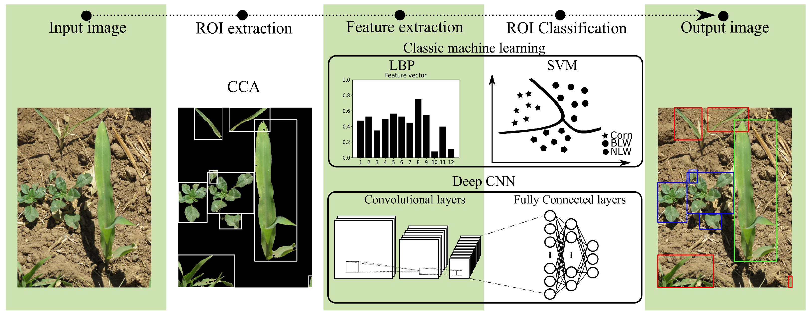
2. Materials and Methods
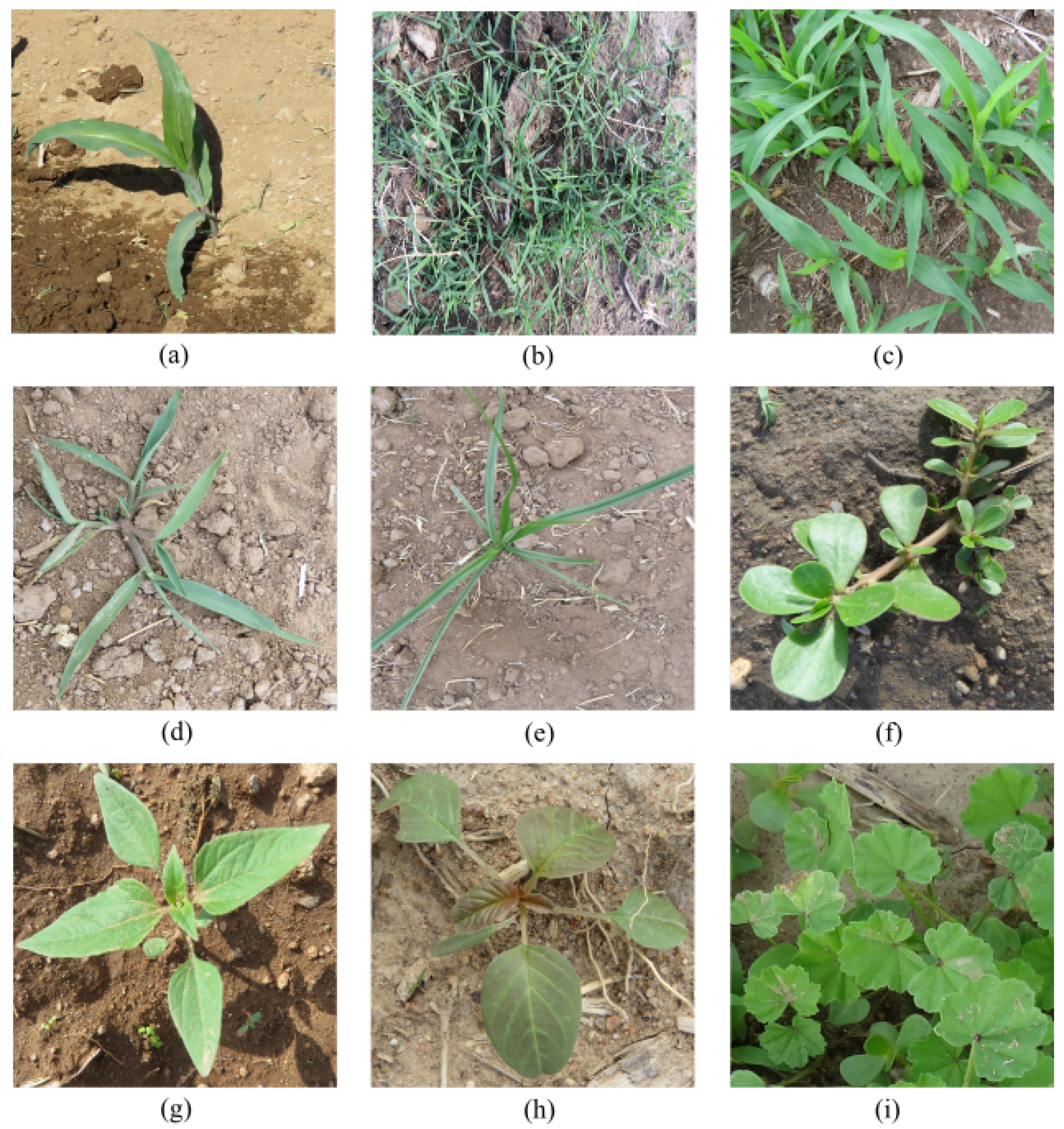
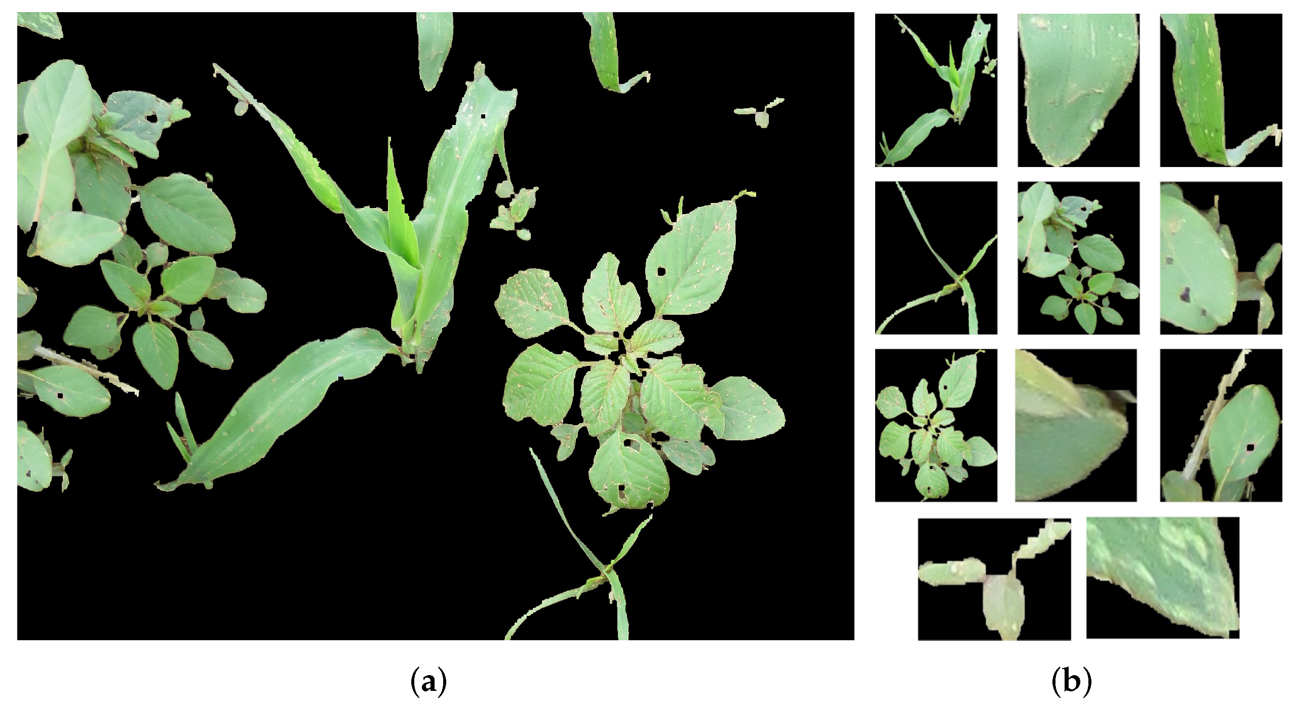
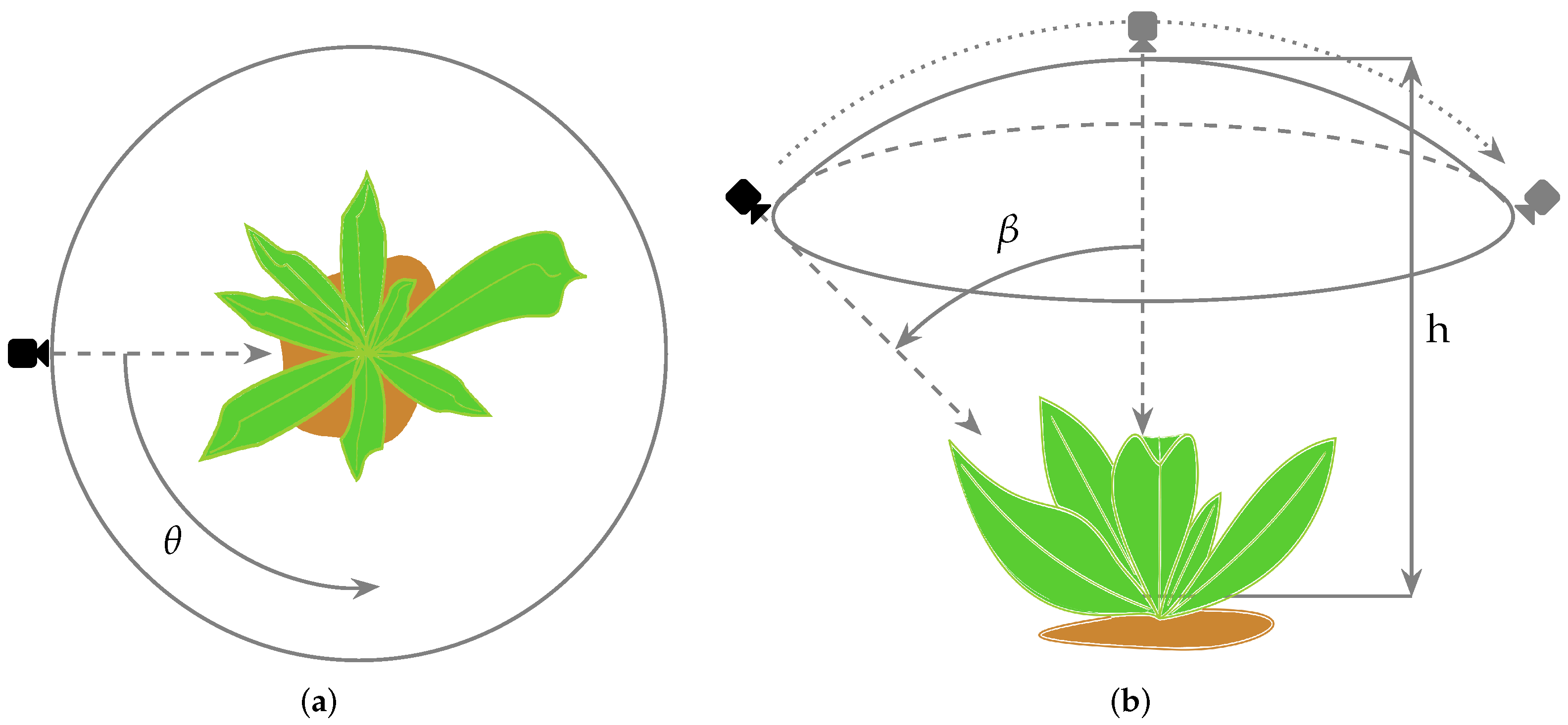
2.1. Dataset Generation and Image Pre-Prossessing
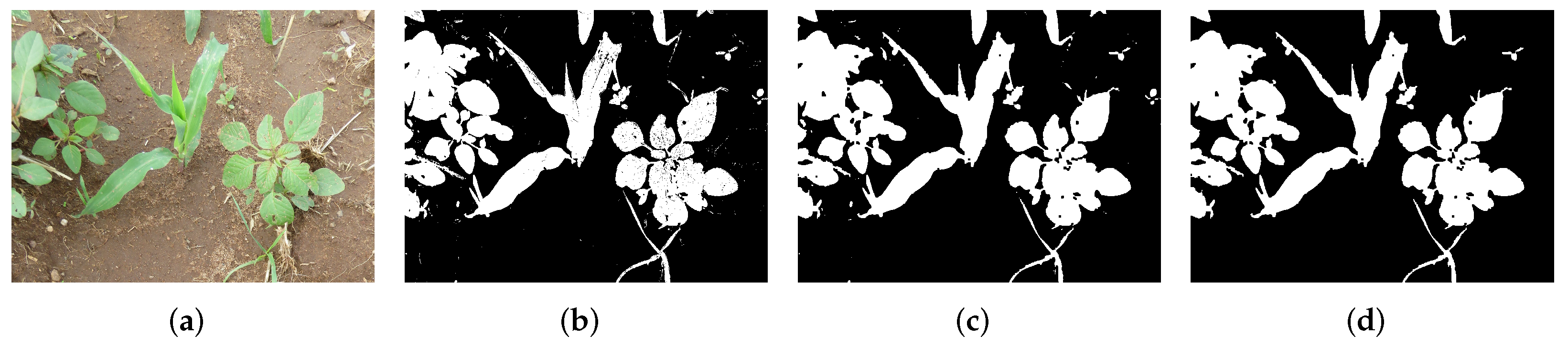
2.1.1. Image Segmentation
2.1.2. Image Enhancement
2.2. Weed and Crop Classification
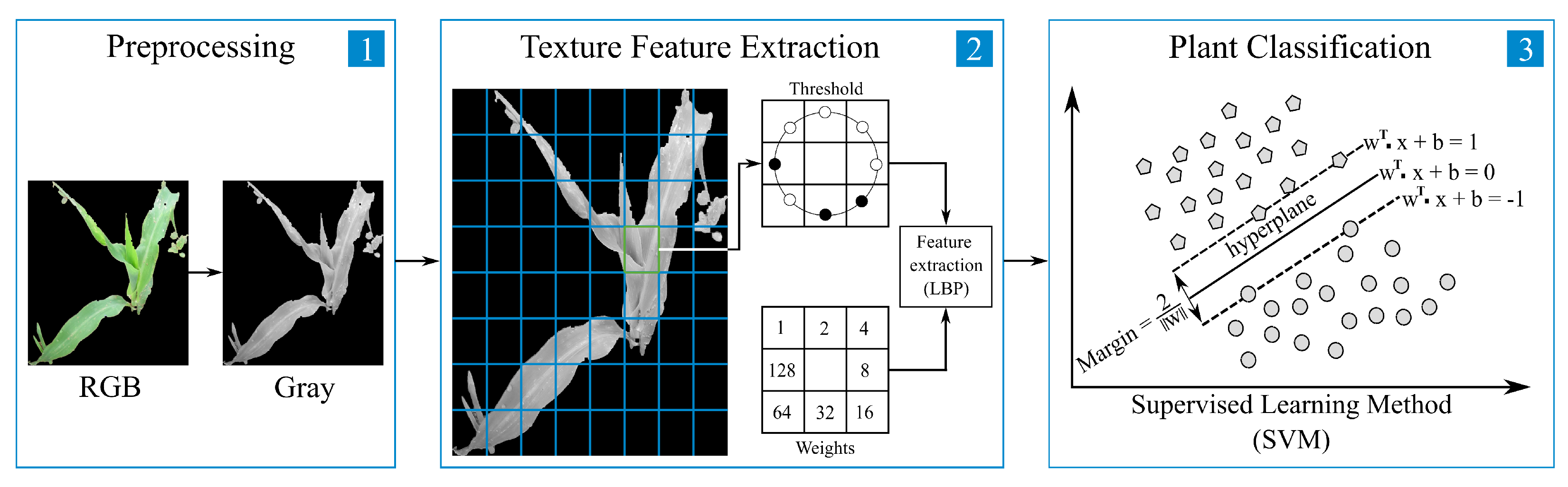
2.2.1. Classical Machine Learning Approach
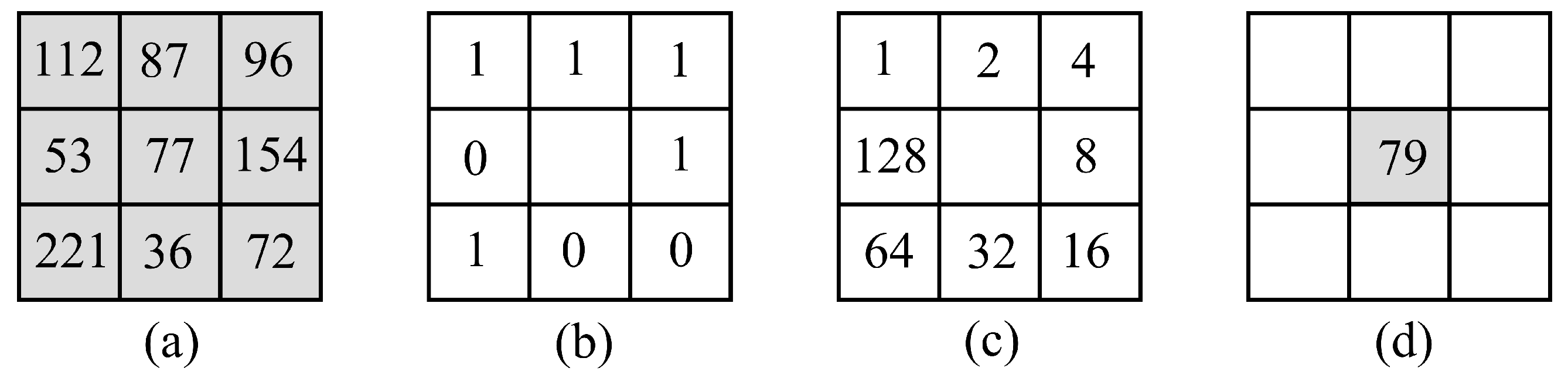
Texture Extraction
SVM Classifier Training Stage
2.2.2. CNN Classification Approach
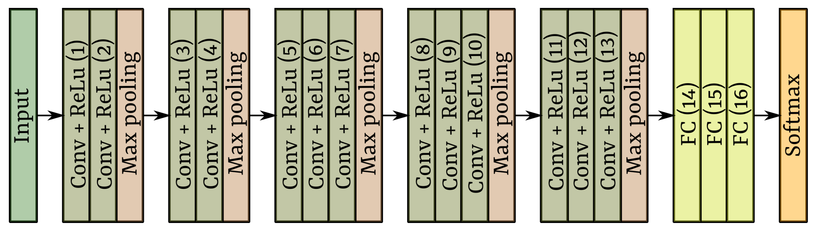
VGG Networks
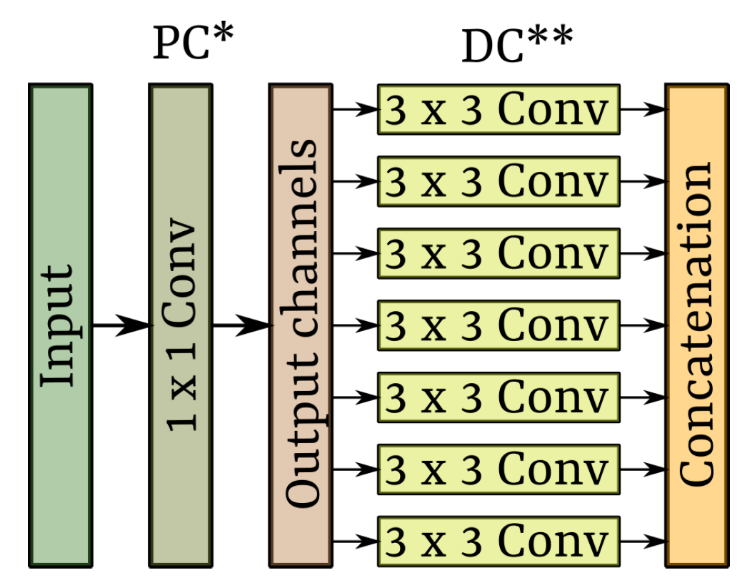
Xception Network
2.3. Performance Evaluation Metrics
3. Results
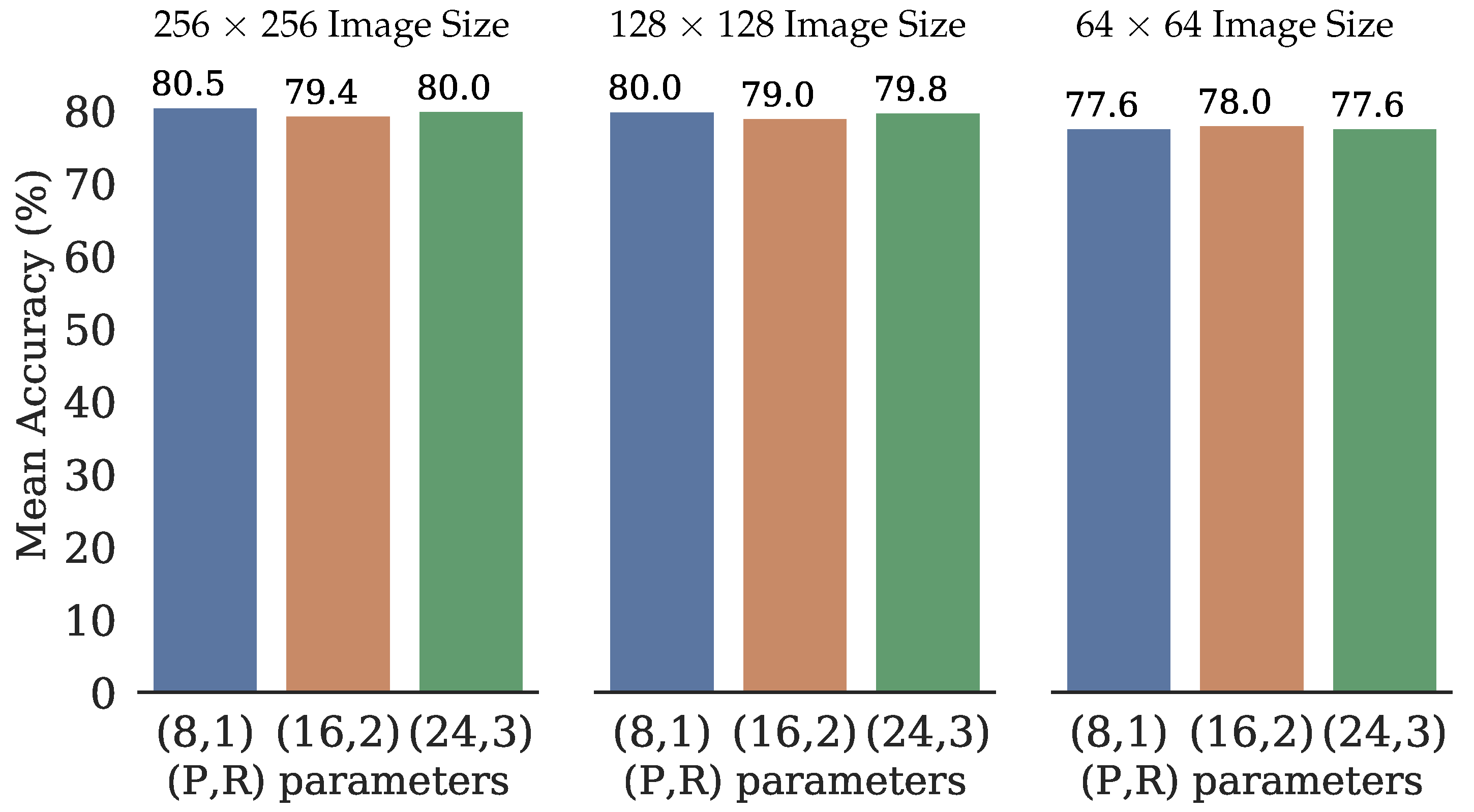
3.1. Classic Machine Learning
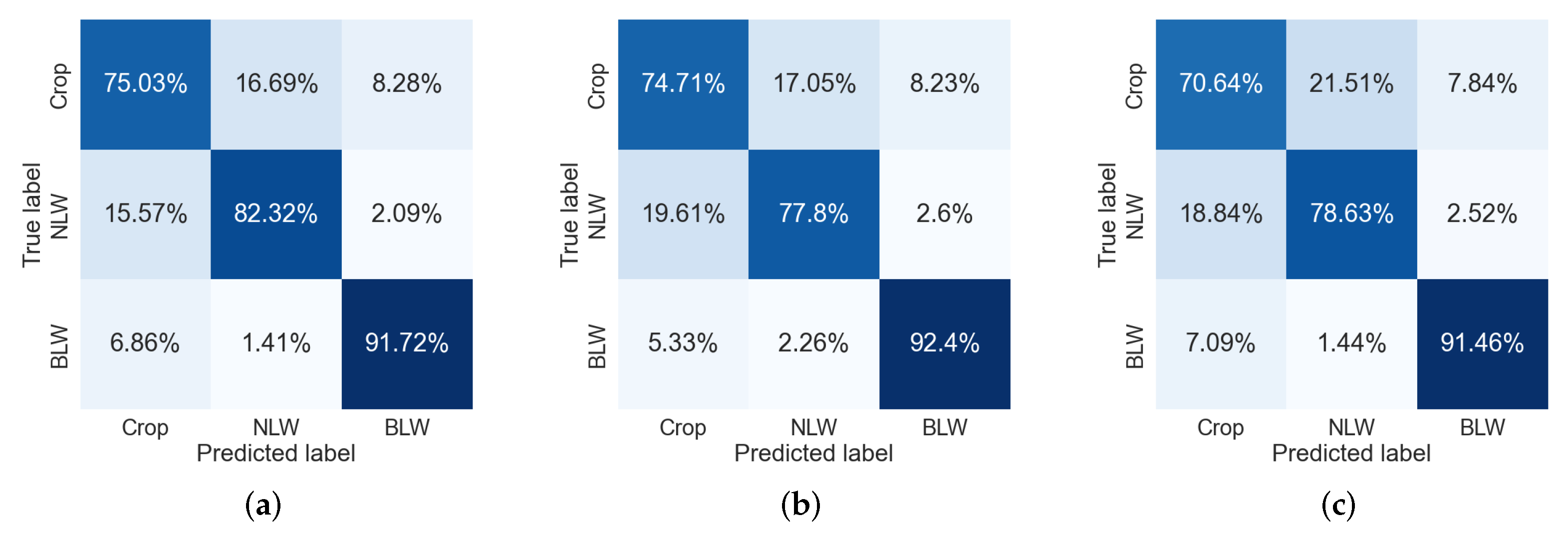
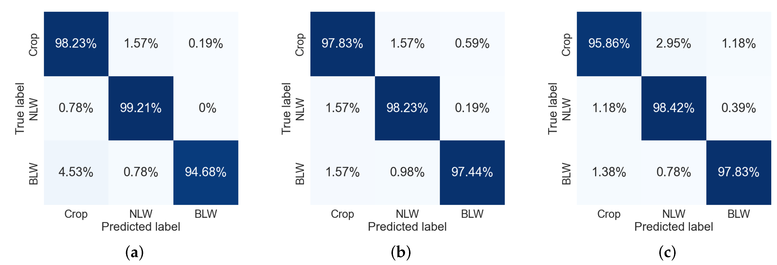
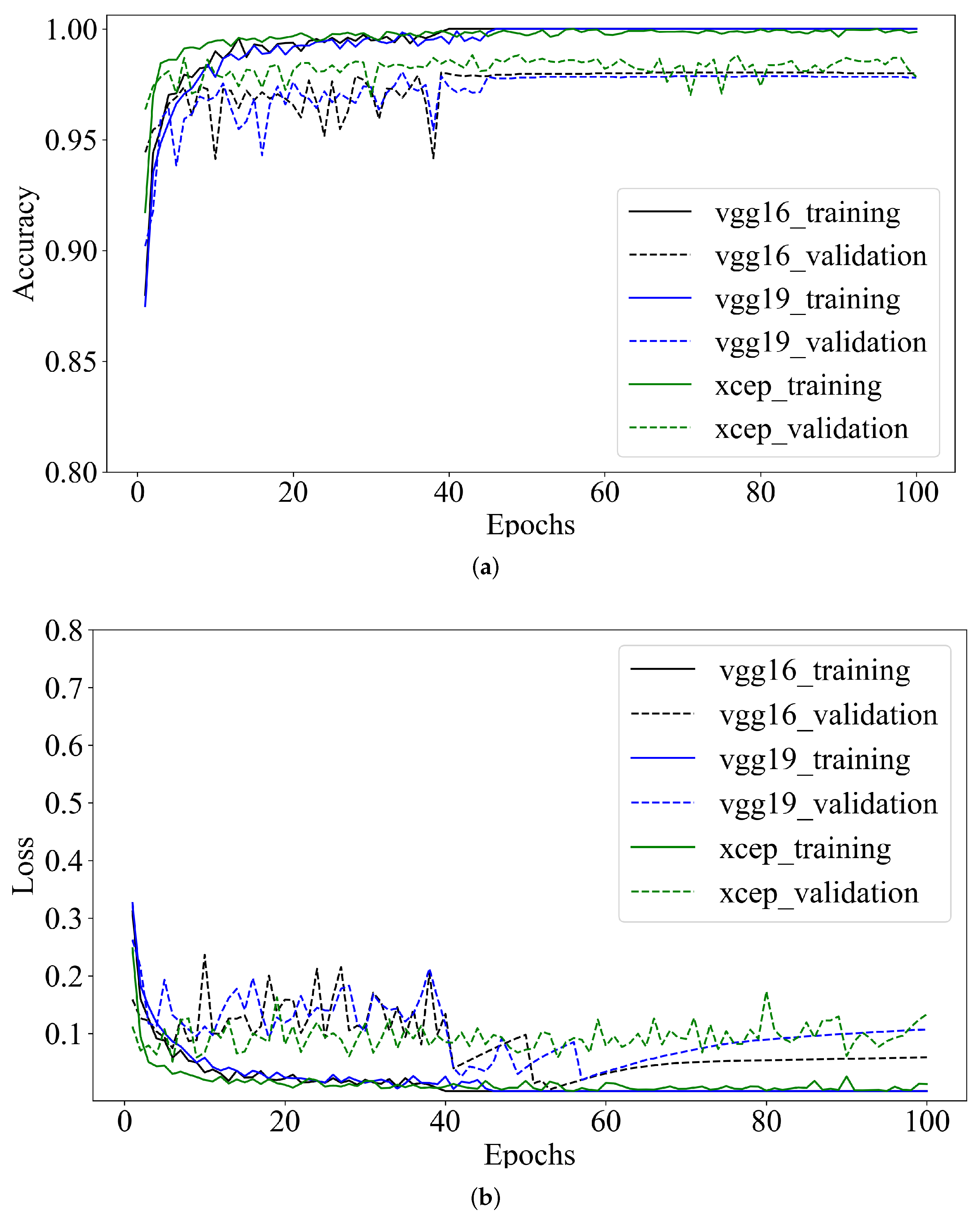
3.2. CNN Classification
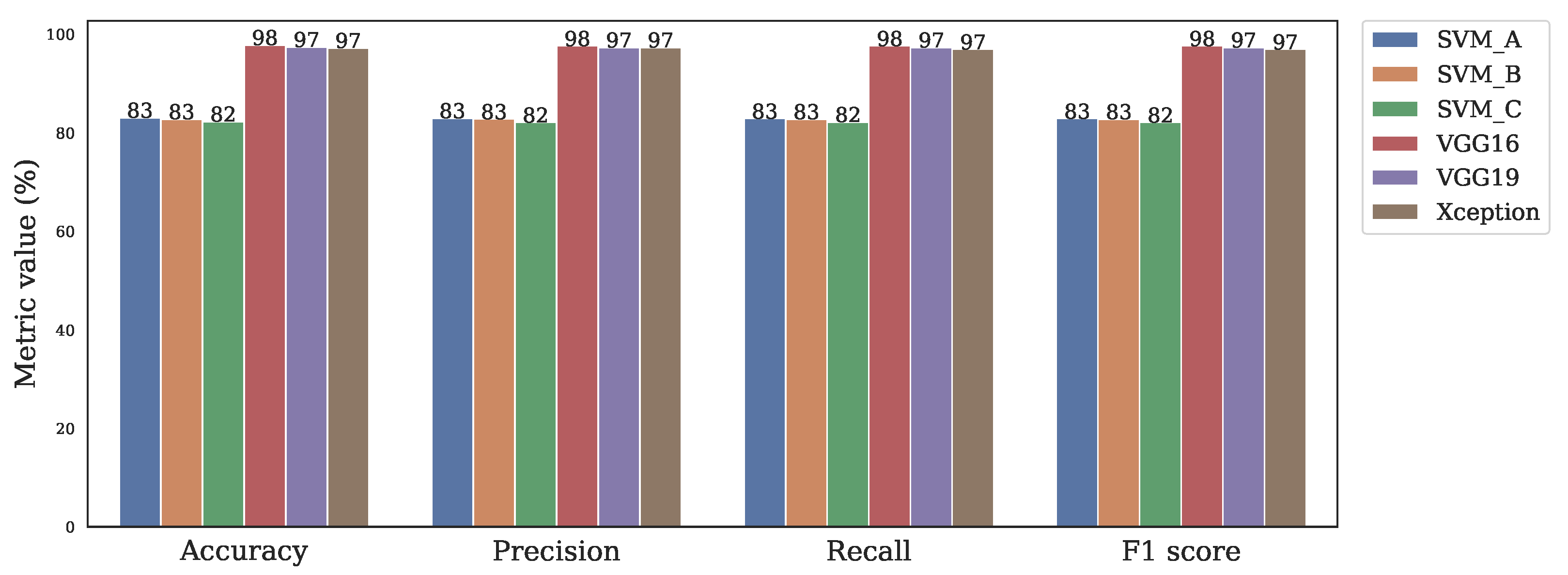
3.3. Comparison of Classic Machine Learning and CNN
4. Discussion
5. Conclusions
Author Contributions
Funding
Institutional Review Board Statement
Informed Consent Statement
Data Availability Statement
Acknowledgments
Conflicts of Interest
References
- Ngoune Tandzi, L.; Mutengwa, C.S.; Ngonkeu, E.L.M.; Gracen, V. Breeding Maize for Tolerance to Acidic Soils: A Review. Agronomy 2018, 8, 84. [Google Scholar] [CrossRef] [Green Version]
- Gao, J.; Nuyttens, D.; Lootens, P.; He, Y.; Pieters, J.G. Recognising weeds in a maize crop using a random forest machine-learning algorithm and near-infrared snapshot mosaic hyperspectral imagery. Biosyst. Eng. 2018, 170, 39–50. [Google Scholar] [CrossRef]
- Yeganehpoor, F.; Salmasi, S.Z.; Abedi, G.; Samadiyan, F.; Beyginiya, V. Effects of cover crops and weed management on corn yield. J. Saudi Soc. Agric. Sci. 2015, 14, 178–181. [Google Scholar] [CrossRef] [Green Version]
- Kamath, R.; Balachandra, M.; Prabhu, S. Crop and weed discrimination using laws’ texture masks. Int. J. Agric. Biol. Eng. 2020, 13, 191–197. [Google Scholar] [CrossRef]
- Hamuda, E.; Glavin, M.; Jones, E. A survey of image processing techniques for plant extraction and segmentation in the field. Comput. Electron. Agric. 2016, 125, 184–199. [Google Scholar] [CrossRef]
- Wang, H.; Liu, W.; Zhao, K.; Yu, H.; Zhang, J.; Wang, J. Evaluation of weed control efficacy and crop safety of the new HPPD-inhibiting herbicide-QYR301. Sci. Rep. 2018, 8, 7910. [Google Scholar] [CrossRef] [Green Version]
- Kamath, R.; Balachandra, M.; Vardhan, A.; Maheshwari, U. Classification of paddy crop and weeds using semantic segmentation. Cogent Eng. 2022, 9, 2018791. [Google Scholar] [CrossRef]
- Louargant, M.; Jones, G.; Faroux, R.; Paoli, J.N.; Maillot, T.; Gée, C.; Villette, S. Unsupervised Classification Algorithm for Early Weed Detection in Row-Crops by Combining Spatial and Spectral Information. Remote Sens. 2018, 10, 761. [Google Scholar] [CrossRef] [Green Version]
- Pott, L.P.; Amado, T.J.; Schwalbert, R.A.; Sebem, E.; Jugulam, M.; Ciampitti, I.A. Pre-planting weed detection based on ground field spectral data. Pest Manag. Sci. 2020, 76, 1173–1182. [Google Scholar] [CrossRef]
- Gerhards, R.; Christensen, S. Real-time weed detection, decision making and patch spraying in maize, sugarbeet, winter wheat and winter barley. Weed Res. 2003, 43, 385–392. [Google Scholar]
- Christensen, S.; Heisel, T.; Walter, A.M.; Graglia, E. A decision algorithm for patch spraying. Weed Res. 2003, 43, 276–284. [Google Scholar] [CrossRef]
- Monteiro, A.; Santos, S. Sustainable Approach to Weed Management: The Role of Precision Weed Management. Agronomy 2022, 12, 118. [Google Scholar] [CrossRef]
- Nikolić, N.; Rizzo, D.; Marraccini, E.; Ayerdi Gotor, A.; Mattivi, P.; Saulet, P.; Persichetti, A.; Masin, R. Site- and time-specific early weed control is able to reduce herbicide use in maize—A case study. Ital. J. Agron. 2021, 16, 1780. [Google Scholar] [CrossRef]
- Wang, A.; Zhang, W.; Wei, X. A review on weed detection using ground-based machine vision and image processing techniques. Comput. Electron. Agric. 2019, 158, 226–240. [Google Scholar] [CrossRef]
- Xu, Y.; He, R.; Gao, Z.; Li, C.; Zhai, Y.; Jiao, Y. Weed Density Detection Method Based on Absolute Feature Corner Points in Field. Agronomy 2020, 10, 113. [Google Scholar] [CrossRef] [Green Version]
- Liu, H.; Sun, H.; Li, M.; Iida, M. Application of Color Featuring and Deep Learning in Maize Plant Detection. Remote Sens. 2020, 12, 2229. [Google Scholar] [CrossRef]
- Pérez-Ortiz, M.; Peña, J.; Gutiérrez, P.; Torres-Sánchez, J.; Hervás-Martínez, C.; López-Granados, F. A semi-supervised system for weed mapping in sunflower crops using unmanned aerial vehicles and a crop row detection method. Appl. Soft Comput. 2015, 37, 533–544. [Google Scholar] [CrossRef]
- Bakhshipour, A.; Jafari, A. Evaluation of support vector machine and artificial neural networks in weed detection using shape features. Comput. Electron. Agric. 2018, 145, 153–160. [Google Scholar] [CrossRef]
- Herrera, P.J.; Dorado, J.; Ribeiro, A. A Novel Approach for Weed Type Classification Based on Shape Descriptors and a Fuzzy Decision-Making Method. Sensors 2014, 14, 15304–15324. [Google Scholar] [CrossRef] [Green Version]
- Wu, Z.; Chen, Y.; Zhao, B.; Kang, X.; Ding, Y. Review of Weed Detection Methods Based on Computer Vision. Sensors 2021, 21, 3647. [Google Scholar] [CrossRef]
- Farooq, A.; Jia, X.; Hu, J.; Zhou, J. Multi-Resolution Weed Classification via Convolutional Neural Network and Superpixel Based Local Binary Pattern Using Remote Sensing Images. Remote Sens. 2019, 11, 1692. [Google Scholar] [CrossRef] [Green Version]
- Nguyen Thanh Le, V.; Apopei, B.; Alameh, K. Effective plant discrimination based on the combination of local binary pattern operators and multiclass support vector machine methods. Inf. Process. Agric. 2019, 6, 116–131. [Google Scholar] [CrossRef]
- Le, V.N.T.; Ahderom, S.; Alameh, K. Performances of the LBP Based Algorithm over CNN Models for Detecting Crops and Weeds with Similar Morphologies. Sensors 2020, 20, 2193. [Google Scholar] [CrossRef] [PubMed]
- Chen, Y.; Wu, Z.; Zhao, B.; Fan, C.; Shi, S. Weed and Corn Seedling Detection in Field Based on Multi Feature Fusion and Support Vector Machine. Sensors 2021, 21, 212. [Google Scholar] [CrossRef]
- Hamouchene, I.; Aouat, S.; Lacheheb, H. Texture Segmentation and Matching Using LBP Operator and GLCM Matrix. In Intelligent Systems for Science and Information: Extended and Selected Results from the Science and Information Conference 2013; Chen, L., Kapoor, S., Bhatia, R., Eds.; Springer International Publishing: Cham, Switzerland, 2014; pp. 389–407. [Google Scholar]
- Krähmer, H.; Walter, H.; Jeschke, P.; Haaf, K.; Baur, P.; Evans, R. What makes a molecule a pre- or a post-herbicide—How valuable are physicochemical parameters for their design? Pest Manag. Sci. 2021, 77, 4863–4873. [Google Scholar] [CrossRef]
- Dadashzadeh, M.; Abbaspour-Gilandeh, Y.; Mesri-Gundoshmian, T.; Sabzi, S.; Hernández-Hernández, J.L.; Hernández-Hernández, M.; Arribas, J.I. Weed Classification for Site-Specific Weed Management Using an Automated Stereo Computer-Vision Machine-Learning System in Rice Fields. Plants 2020, 9, 559. [Google Scholar] [CrossRef]
- Montes de Oca, A.; Flores, G. A UAS equipped with a thermal imaging system with temperature calibration for Crop Water Stress Index computation. In Proceedings of the 2021 International Conference on Unmanned Aircraft Systems (ICUAS), Athens, Greece, 15–18 June 2021; pp. 714–720. [Google Scholar]
- Pulido, C.; Solaque, L.; Velasco, N. Weed recognition by SVM texture feature classification in outdoor vegetable crop images. Ing. Investig. 2017, 37, 68–74. [Google Scholar] [CrossRef]
- Montes de Oca, A.; Flores, G. The AgriQ: A low-cost unmanned aerial system for precision agriculture. Expert Syst. Appl. 2021, 182, 115163. [Google Scholar] [CrossRef]
- de Oca, A.M.; Arreola, L.; Flores, A.; Sanchez, J.; Flores, G. Low-cost multispectral imaging system for crop monitoring. In Proceedings of the 2018 International Conference on Unmanned Aircraft Systems (ICUAS), Dallas, TX, USA, 12–15 June 2018; pp. 443–451. [Google Scholar]
- Krizhevsky, A.; Sutskever, I.; Hinton, G.E. ImageNet Classification with Deep Convolutional Neural Networks. In Advances in Neural Information Processing Systems; Pereira, F., Burges, C.J.C., Bottou, L., Weinberger, K.Q., Eds.; Curran Associates, Inc.: Lake Tahoe, NV, USA, 2012; Volume 25. [Google Scholar]
- dos Santos Ferreira, A.; Matte Freitas, D.; Gonçalves da Silva, G.; Pistori, H.; Theophilo Folhes, M. Weed detection in soybean crops using ConvNets. Comput. Electron. Agric. 2017, 143, 314–324. [Google Scholar] [CrossRef]
- Ahmad, A.; Saraswat, D.; Aggarwal, V.; Etienne, A.; Hancock, B. Performance of deep learning models for classifying and detecting common weeds in corn and soybean production systems. Comput. Electron. Agric. 2021, 184, 106081. [Google Scholar] [CrossRef]
- Haralick, R.M.; Shapiro, L.G. Computer and Robot Vision, Vol. 1, 1st ed.; Addison-Wesley Publishing Company, Inc.: Boston, MA, USA, 1992; p. 672. [Google Scholar]
- He, L.; Ren, X.; Gao, Q.; Zhao, X.; Yao, B.; Chao, Y. The connected-component labeling problem: A review of state-of-the-art algorithms. Pattern Recognit. 2017, 70, 25–43. [Google Scholar] [CrossRef]
- Simonyan, K.; Zisserman, A. Very deep convolutional networks for large-scale image recognition. In Proceedings of the 3rd International Conference on Learning Representations, San Diego, CA, USA, 7–9 May 2015. [Google Scholar]
- Chollet, F. Xception: Deep learning with depthwise separable convolutions. In Proceedings of the IEEE Conference on Computer Vision and Pattern Recognition (CVPR), Honolulu, HI, USA, 21–26 July 2017; pp. 1800–1807. [Google Scholar]
- Ojala, T.; Pietikainen, M.; Maenpaa, T. Multiresolution gray-scale and rotation invariant texture classification with local binary patterns. IEEE Trans. Pattern Anal. Mach. Intell. 2002, 24, 971–987. [Google Scholar] [CrossRef]
- Cheng, H.; Jiang, X.; Sun, Y.; Wang, J. Color image segmentation: Advances and prospects. Pattern Recognit. 2001, 34, 2259–2281. [Google Scholar] [CrossRef]
- Yang, W.; Wang, S.; Zhao, X.; Zhang, J.; Feng, J. Greenness identification based on HSV decision tree. Inf. Process. Agric. 2015, 2, 149–160. [Google Scholar] [CrossRef] [Green Version]
- Le, V.N.T.; Ahderom, S.; Apopei, B.; Alameh, K. A novel method for detecting morphologically similar crops and weeds based on the combination of contour masks and filtered Local Binary Pattern operators. GigaScience 2020, 9, giaa017. [Google Scholar] [CrossRef] [Green Version]
- González, R.C.; Woods, R.E. Digital Image Processing, fourth ed.; Pearson: New York, NY, USA, 2018. [Google Scholar]
- George, M.; Zwiggelaar, R. Comparative Study on Local Binary Patterns for Mammographic Density and Risk Scoring. J. Imaging 2019, 5, 24. [Google Scholar] [CrossRef] [Green Version]
- Bishop, C.M. Pattern Recognition and Machine Learning (Information Science and Statistics); Springer: Berlin/Heidelberg, Germany, 2006. [Google Scholar]
- Alzubaidi, L.; Zhang, J.; Humaidi, A.J.; Al-Dujaili, A.; Duan, Y.; Al-Shamma, O.; Santamaría, J.; Fadhel, M.A.; Al-Amidie, M.; Farhan, L. Review of deep learning: Concepts, CNN architectures, challenges, applications, future directions. J. Big Data 2021, 8, 1–74. [Google Scholar] [CrossRef]
- Khan, S.; Rahmani, H.; Shah, S.A.A.; Bennamoun, M. A Guide to Convolutional Neural Networks for Computer Vision. Synth. Lect. Comput. Vis. 2018, 8, 1–207. [Google Scholar] [CrossRef]
- Gad, A.F. Practical Computer Vision Applications Using Deep Learning with CNNs: With Detailed Examples in Python Using TensorFlow and Kivy, 1st ed.; Apress: Menoufia, Egypt, 2018. [Google Scholar]
- Espejo-Garcia, B.; Mylonas, N.; Athanasakos, L.; Fountas, S.; Vasilakoglou, I. Towards weeds identification assistance through transfer learning. Comput. Electron. Agric. 2020, 171, 105306. [Google Scholar] [CrossRef]
- Theckedath, D.; Sedamkar, R.R. Detecting Affect States Using VGG16, ResNet50 and SE ResNet50 Networks. SN Comput. Sci. 2020, 1, 79. [Google Scholar] [CrossRef] [Green Version]
- Szegedy, C.; Liu, W.; Jia, Y.; Sermanet, P.; Reed, S.; Anguelov, D.; Erhan, D.; Vanhoucke, V.; Rabinovich, A. Going Deeper with Convolutions. In Proceedings of the IEEE Conference on Computer Vision and Pattern Recognition (CVPR), Boston, MA, USA, 7–12 June 2015; pp. 1–9. [Google Scholar]
- Szegedy, C.; Ioffe, S.; Vanhoucke, V.; Alemi, A. Inception-v4, Inception-ResNet and the Impact of Residual Connections on Learning. In Proceedings of the Thirty-First AAAI Conference on Artificial Intelligence, San Francisco, CA, USA, 4–9 February 2017. [Google Scholar]
- Peteinatos, G.G.; Reichel, P.; Karouta, J.; Andújar, D.; Gerhards, R. Weed Identification in Maize, Sunflower, and Potatoes with the Aid of Convolutional Neural Networks. Remote Sens. 2020, 12, 4185. [Google Scholar] [CrossRef]
- Holt, J.S. Herbicides. In Encyclopedia of Biodiversity, 2nd ed.; Levin, S.A., Ed.; Academic Press: Oxford, UK, 2013; pp. 87–95. [Google Scholar]
- Janahiraman, T.V.; Yee, L.K.; Der, C.S.; Aris, H. Leaf Classification using Local Binary Pattern and Histogram of Oriented Gradients. In Proceedings of the 2019 seventh International Conference on Smart Computing & Communications (ICSCC), Sarawak, Malaysia, 28–30 June 2019; pp. 1–5. [Google Scholar]
- Wu, S.G.; Bao, F.S.; Xu, E.Y.; Wang, Y.X.; Chang, Y.F.; Xiang, Q.L. A Leaf Recognition Algorithm for Plant Classification Using Probabilistic Neural Network. In Proceedings of the 2007 IEEE International Symposium on Signal Processing and Information Technology, Giza, Egypt, 15–18 December 2007; pp. 11–16. [Google Scholar]
- Jiang, H.; Zhang, C.; Qiao, Y.; Zhang, Z.; Zhang, W.; Song, C. CNN feature based graph convolutional network for weed and crop recognition in smart farming. Comput. Electron. Agric. 2020, 174, 105450. [Google Scholar] [CrossRef]
- Dyrmann, M.; Karstoft, H.; Midtiby, H.S. Plant species classification using deep convolutional neural network. Biosyst. Eng. 2016, 151, 72–80. [Google Scholar] [CrossRef]
- Olsen, A.; Konovalov, D.A.; Philippa, B.; Ridd, P.; Wood, J.C.; Johns, J.; Banks, W.; Girgenti, B.; Kenny, O.; Whinney, J.; et al. DeepWeeds: A Multiclass Weed Species Image Dataset for Deep Learning. Sci. Rep. 2019, 9, 2058. [Google Scholar] [CrossRef] [PubMed]
- Yu, J.; Sharpe, S.M.; Schumann, A.W.; Boyd, N.S. Detection of broadleaf weeds growing in turfgrass with convolutional neural networks. Pest Manag. Sci. 2019, 75, 2211–2218. [Google Scholar] [CrossRef] [PubMed]
- dos Santos Ferreira, A.; Freitas, D.M.; da Silva, G.G.; Pistori, H.; Folhes, M.T. Unsupervised deep learning and semi-automatic data labeling in weed discrimination. Comput. Electron. Agric. 2019, 165, 104963. [Google Scholar] [CrossRef]
- Jadhav, S.B.; Udupi, V.R.; Patil, S.B. Identification of plant diseases using convolutional neural networks. Int. J. Inf. Tecnol. 2021, 13, 2461–2470. [Google Scholar] [CrossRef]
- Sarki, R.; Ahmed, K.; Wang, H.; Zhang, Y.; Wang, K. Automated detection of COVID-19 through convolutional neural network using chest x-ray images. PLoS ONE 2022, 17, e0262052. [Google Scholar] [CrossRef]
- Glowacz, A. Thermographic Fault Diagnosis of Ventilation in BLDC Motors. Sensors 2021, 21, 7245. [Google Scholar] [CrossRef]


| Class | Scientific Name | Common Name | Number of Instances |
|---|---|---|---|
| Crop | Zea mays L. | Corn | 5080 |
| NLW | Cynodon dactylon | Bermudagrass | 5080 |
| Eleusine indica | Goosegrass | ||
| Digitaria sanguinalis | Large crabgrass | ||
| Cyperus esculentus | Yellow Nutsedge | ||
| BLW | Portulaca oleracea | Common Purslane | 5080 |
| Tithonia tubaeformis (Jacq.) Cass. | – | ||
| Amaranthus spinosus | Spiny Amaranth | ||
| Malva parviflora | Little Mallow |
| Image Size | Cell Size | |||||
|---|---|---|---|---|---|---|
| 8 × 8 | 16 × 16 | 32 × 32 | 64 × 64 | 128 × 128 | ||
| P = 8, R = 1 | 256 × 256 | √ | √ | √ | √ | √ |
| 128 × 128 | √ | √ | √ | √ | ||
| 64 × 64 | √ | √ | √ | |||
| P = 16, R = 2 | 256 × 256 | √ | √ | √ | √ | √ |
| 128 × 128 | √ | √ | √ | √ | ||
| 64 × 64 | √ | √ | √ | |||
| P = 24, R = 3 | 256 × 256 | √ | √ | √ | √ | √ |
| 128 × 128 | √ | √ | √ | √ | ||
| 64 × 64 | √ | √ | √ | |||
| Metrics | 256 × 256 Image | 128 × 128 Image | 64 × 64 Image | ||||||||||
|---|---|---|---|---|---|---|---|---|---|---|---|---|---|
| Cell Size | Cell Size | Cell Size | |||||||||||
| 8 × 8 | 16 × 16 | 32 × 32 | 64 × 64 | 128 × 128 | 8 × 8 | 16 × 16 | 32 × 32 | 64 × 64 | 8 × 8 | 16 × 16 | 32 × 32 | ||
| (8,1) | Accuracy (%) | 79.39 | 79.39 | 83.04 | 81.50 | 79.28 | 77.34 | 80.31 | 81.82 | 80.35 | 77.60 | 78.32 | 77.01 |
| Precision (%) | 79.82 | 79.73 | 82.94 | 81.44 | 78.95 | 77.50 | 80.23 | 81.65 | 80.22 | 77.64 | 78.22 | 76.74 | |
| Recall (%) | 79.40 | 79.41 | 82.90 | 81.59 | 79.16 | 77.30 | 80.22 | 81.72 | 80.31 | 77.75 | 78.27 | 76.93 | |
| score (%) | 79.54 | 79.54 | 82.91 | 81.50 | 79.03 | 77.39 | 80.21 | 81.65 | 80.21 | 77.68 | 78.24 | 76.81 | |
| Test time (ms) | 407.65 | 235.57 | 212.07 | 206.46 | 205.03 | 227.98 | 211.58 | 204.57 | 200.28 | 205.70 | 199.77 | 198.25 | |
| (16,2) | Accuracy (%) | 79.72 | 79.3 | 81.36 | 79.96 | 76.5 | 77.54 | 80.53 | 79.65 | 78.45 | 77.08 | 80.31 | 76.73 |
| Precision (%) | 80.02 | 79.96 | 81.23 | 79.69 | 76.03 | 77.69 | 80.70 | 79.72 | 78.52 | 77.07 | 80.27 | 76.71 | |
| Recall (%) | 79.75 | 79.40 | 81.34 | 79.82 | 76.37 | 77.29 | 80.64 | 79.88 | 78.63 | 77.14 | 80.33 | 76.05 | |
| score (%) | 79.87 | 79.57 | 81.27 | 79.74 | 76.13 | 77.42 | 80.67 | 79.73 | 78.58 | 77.10 | 80.30 | 76.86 | |
| Test time (ms) | 439.53 | 250.37 | 221.68 | 215.32 | 213.08 | 241.71 | 210.24 | 202.42 | 202.20 | 207.66 | 200.71 | 199.02 | |
| (24,3) | Accuracy (%) | 77.07 | 80.77 | 82.76 | 81.27 | 78.12 | 77.93 | 81.34 | 82.26 | 77.62 | 76.99 | 78.78 | 77.16 |
| Precision (%) | 77.56 | 81.20 | 82.80 | 81.10 | 77.69 | 78.17 | 81.40 | 82.13 | 77.60 | 77.30 | 78.73 | 77.79 | |
| Recall (%) | 77.08 | 80.82 | 82.77 | 81.20 | 77.90 | 77.90 | 81.38 | 82.18 | 77.76 | 77.02 | 78.93 | 77.10 | |
| score (%) | 77.19 | 80.97 | 82.78 | 81.14 | 77.77 | 78.01 | 81.38 | 82.14 | 77.67 | 77.11 | 78.76 | 76.90 | |
| Test time (ms) | 461.86 | 263.72 | 228.92 | 220.50 | 217.75 | 257.94 | 217.10 | 210.18 | 203.83 | 220.46 | 205.14 | 200.28 | |
| Model | Accuracy (%) | Precision (%) | Recall (%) | Score (%) | Test Time (ms) |
|---|---|---|---|---|---|
| VGG16 | 97.83 | 97.67 | 97.67 | 97.67 | 194.56 |
| VGG19 | 97.44 | 97.33 | 97.33 | 97.33 | 226.96 |
| Xception | 97.24 | 97.33 | 97.00 | 97.00 | 144.38 |
Publisher’s Note: MDPI stays neutral with regard to jurisdictional claims in published maps and institutional affiliations. |
© 2022 by the authors. Licensee MDPI, Basel, Switzerland. This article is an open access article distributed under the terms and conditions of the Creative Commons Attribution (CC BY) license (https://creativecommons.org/licenses/by/4.0/).
Share and Cite
Garibaldi-Márquez, F.; Flores, G.; Mercado-Ravell, D.A.; Ramírez-Pedraza, A.; Valentín-Coronado, L.M. Weed Classification from Natural Corn Field-Multi-Plant Images Based on Shallow and Deep Learning. Sensors 2022, 22, 3021. https://doi.org/10.3390/s22083021
Garibaldi-Márquez F, Flores G, Mercado-Ravell DA, Ramírez-Pedraza A, Valentín-Coronado LM. Weed Classification from Natural Corn Field-Multi-Plant Images Based on Shallow and Deep Learning. Sensors. 2022; 22(8):3021. https://doi.org/10.3390/s22083021
Chicago/Turabian StyleGaribaldi-Márquez, Francisco, Gerardo Flores, Diego A. Mercado-Ravell, Alfonso Ramírez-Pedraza, and Luis M. Valentín-Coronado. 2022. "Weed Classification from Natural Corn Field-Multi-Plant Images Based on Shallow and Deep Learning" Sensors 22, no. 8: 3021. https://doi.org/10.3390/s22083021
APA StyleGaribaldi-Márquez, F., Flores, G., Mercado-Ravell, D. A., Ramírez-Pedraza, A., & Valentín-Coronado, L. M. (2022). Weed Classification from Natural Corn Field-Multi-Plant Images Based on Shallow and Deep Learning. Sensors, 22(8), 3021. https://doi.org/10.3390/s22083021