
Derivative-Free Power Flow Solution for Bipolar DC Networks with Multiple Constant Power Terminals


Abstract
:1. Introduction
2. Power Flow Formulation
3. Iterative Solution
| Algorithm 1: Power flow solution using the triangular-based formulation for multiple constant power loads. |
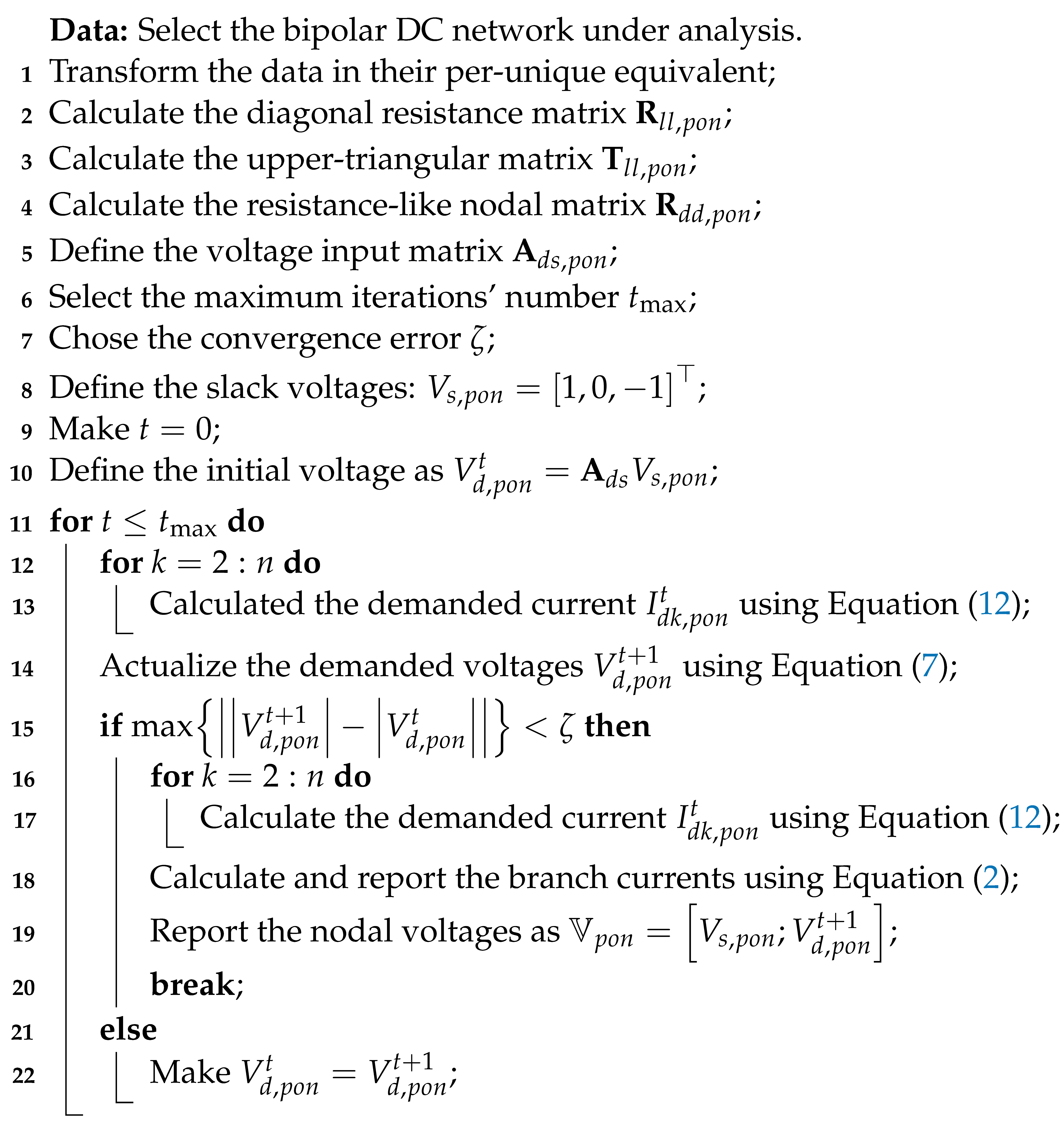 |
4. Test Feeders
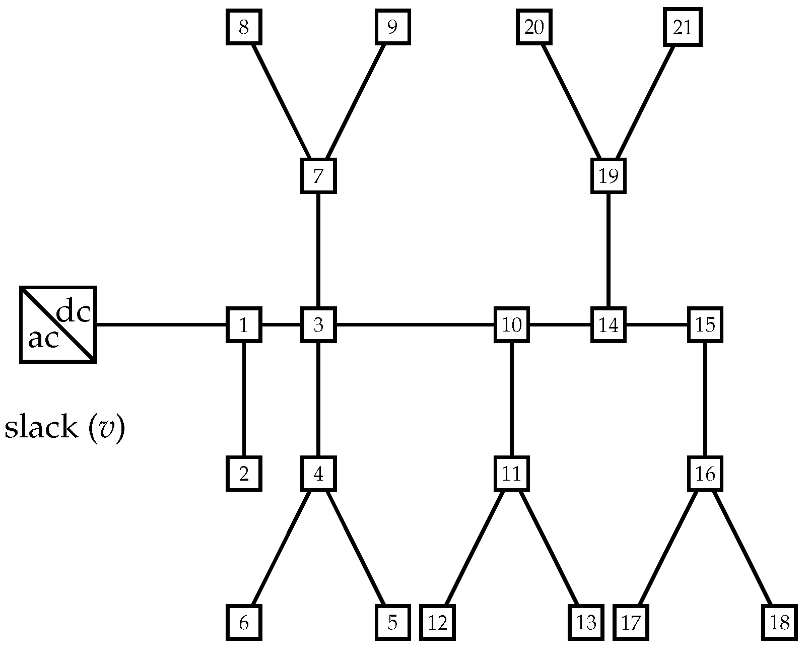
4.1. 21-Bus System
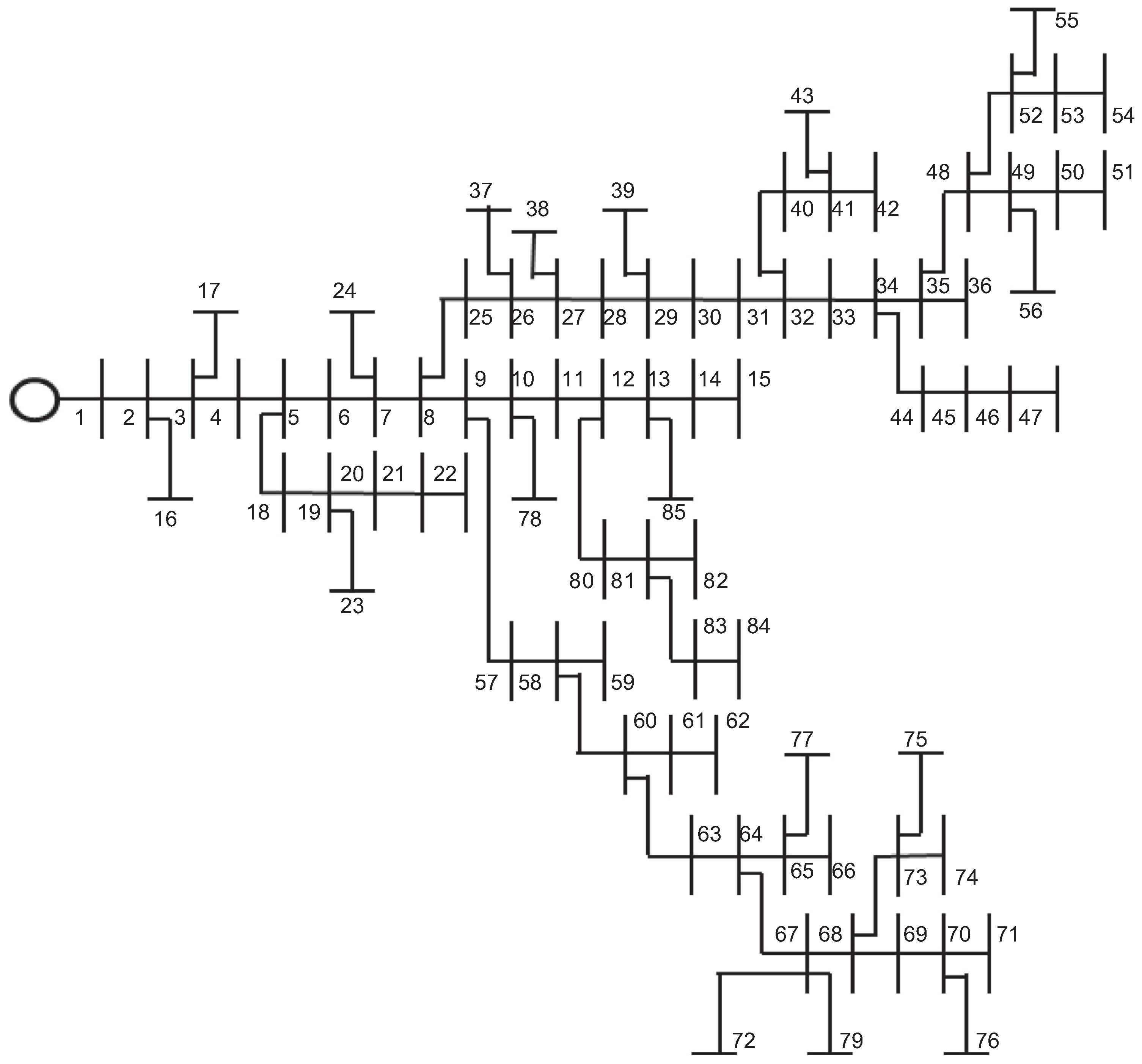
4.2. 85-Bus System
5. Numerical Validations
5.1. Results in the 21-Bus System
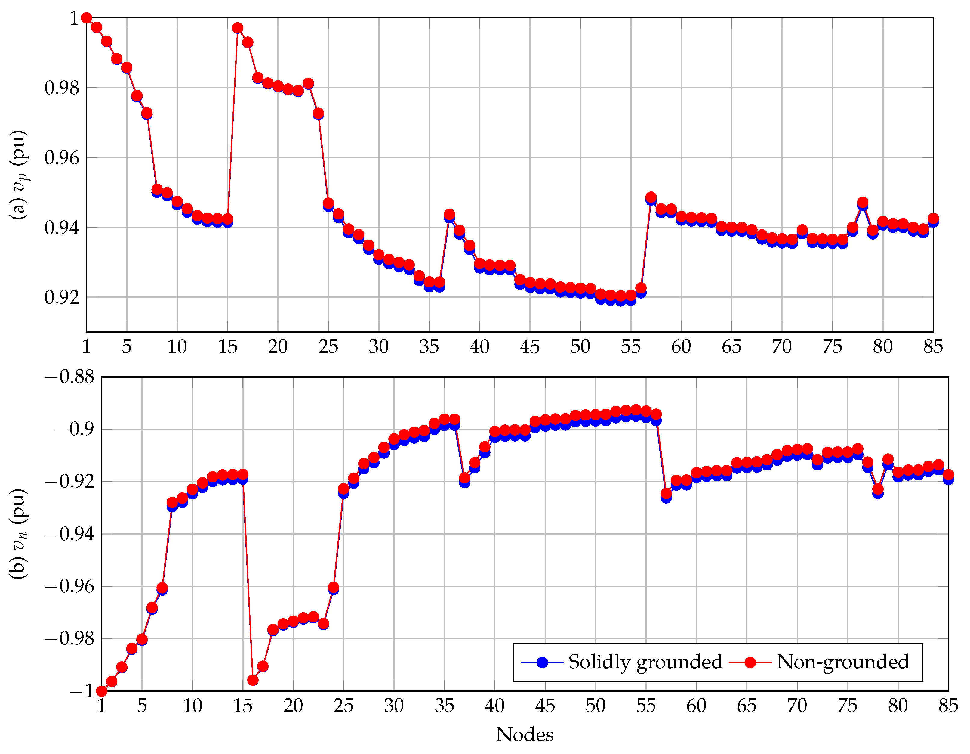
5.2. Results in the 85-Bus Grid
5.3. Complementary Analysis
- ✔
- In the solidly grounded scenario after 1000 consecutive evaluations of the power flow methodology, the average processing times for the 21- and 85-bus grids were 0.6498 ms and 6.4858 ms, respectively. In the non-grounded case, these times were and 6.7226 ms. Note that the increments in these times are expected since the number of iterations increases in the non-grounded neutral wire simulation scenario.
- ✔
- Comparative simulations with the classical backward/forward power flow method adapted for bipolar DC grids demonstrated that both methodologies reach the same voltage profiles and power losses calculations. However, the main advantage of the triangular-based power flow method is the processing time required, since for both tests feeders were 20 % faster than the backward/forward power flow method, which confirmed the results presented by authors of [15] in the case of monopolar DC grid equivalents.
6. Conclusions and Future Works
Author Contributions
Funding
Institutional Review Board Statement
Informed Consent Statement
Data Availability Statement
Conflicts of Interest
References
- Mackay, L.; Blij, N.H.v.d.; Ramirez-Elizondo, L.; Bauer, P. Toward the universal DC distribution system. Electr. Power Components Syst. 2017, 45, 1032–1042. [Google Scholar] [CrossRef] [Green Version]
- Montoya, O.D. Numerical Approximation of the Maximum Power Consumption in DC-MGs With CPLs via an SDP Model. IEEE Trans. Circuits Syst. II Express Briefs 2019, 66, 642–646. [Google Scholar] [CrossRef]
- Parhizi, S.; Lotfi, H.; Khodaei, A.; Bahramirad, S. State of the Art in Research on Microgrids: A Review. IEEE Access 2015, 3, 890–925. [Google Scholar] [CrossRef]
- Siraj, K.; Khan, H.A. DC distribution for residential power networks—A framework to analyze the impact of voltage levels on energy efficiency. Energy Rep. 2020, 6, 944–951. [Google Scholar] [CrossRef]
- Li, B.; Wang, W.; Liu, Y.; Li, B.; Wen, W. Research on power flow calculation method of true bipolar VSC-HVDC grids with different operation modes and control strategies. Int. J. Electr. Power Energy Syst. 2021, 126, 106558. [Google Scholar] [CrossRef]
- Zhu, H.; Zhu, M.; Zhang, J.; Cai, X.; Dai, N. Topology and operation mechanism of monopolarto-bipolar DC-DC converter interface for DC grid. In Proceedings of the 2016 IEEE 8th International Power Electronics and Motion Control Conference (IPEMC-ECCE Asia), Hefei, China, 22–26 May 2016. [Google Scholar] [CrossRef]
- Guo, C.; Wang, Y.; Liao, J. Coordinated Control of Voltage Balancers for the Regulation of Unbalanced Voltage in a Multi-Node Bipolar DC Distribution Network. Electronics 2022, 11, 166. [Google Scholar] [CrossRef]
- Garces, A. Uniqueness of the power flow solutions in low voltage direct current grids. Electr. Power Syst. Res. 2017, 151, 149–153. [Google Scholar] [CrossRef]
- Chew, B.S.H.; Xu, Y.; Wu, Q. Voltage balancing for bipolar DC distribution grids: A power flow based binary integer multi-objective optimization approach. IEEE Trans. Power Syst. 2018, 34, 28–39. [Google Scholar] [CrossRef] [Green Version]
- Lee, J.O.; Kim, Y.S.; Moon, S.I. Current Injection Power Flow Analysis and Optimal Generation Dispatch for Bipolar DC Microgrids. IEEE Trans. Smart Grid 2021, 12, 1918–1928. [Google Scholar] [CrossRef]
- Rivera, S.; Lizana, R.; Kouro, S.; Dragičević, T.; Wu, B. Bipolar dc power conversion: State-of-the-art and emerging technologies. IEEE J. Emerg. Sel. Top. Power Electron. 2020, 9, 1192–1204. [Google Scholar] [CrossRef]
- Litrán, S.P.; Durán, E.; Semião, J.; Barroso, R.S. Single-Switch Bipolar Output DC-DC Converter for Photovoltaic Application. Electronics 2020, 9, 1171. [Google Scholar] [CrossRef]
- Javid, Z.; Karaagac, U.; Kocar, I.; Chan, K.W. Laplacian Matrix-Based Power Flow Formulation for LVDC Grids with Radial and Meshed Configurations. Energies 2021, 14, 1866. [Google Scholar] [CrossRef]
- Simpson-Porco, J.W.; Dorfler, F.; Bullo, F. On Resistive Networks of Constant-Power Devices. IEEE Trans. Circuits Syst. II Express Briefs 2015, 62, 811–815. [Google Scholar] [CrossRef] [Green Version]
- Montoya, O.D.; Gil-González, W.; Garces, A. Numerical methods for power flow analysis in DC networks: State of the art, methods and challenges. Int. J. Electr. Power Energy Syst. 2020, 123, 106299. [Google Scholar] [CrossRef]
- Montoya, O.D.; Grisales-Norena, L.F.; Gil-Gonzalez, W. Triangular Matrix Formulation for Power Flow Analysis in Radial DC Resistive Grids With CPLs. IEEE Trans. Circuits Syst. II Express Briefs 2020, 67, 1094–1098. [Google Scholar] [CrossRef]
- Kim, J.; Cho, J.; Kim, H.; Cho, Y.; Lee, H. Power Flow Calculation Method of DC Distribution Network for Actual Power System. KEPCO J. Electr. Power Energy 2020, 6, 419–425. [Google Scholar] [CrossRef]
- Mackay, L.; Guarnotta, R.; Dimou, A.; Morales-Espana, G.; Ramirez-Elizondo, L.; Bauer, P. Optimal Power Flow for Unbalanced Bipolar DC Distribution Grids. IEEE Access 2018, 6, 5199–5207. [Google Scholar] [CrossRef]
- Garces, A. On the Convergence of Newton’s Method in Power Flow Studies for DC Microgrids. IEEE Trans. Power Syst. 2018, 33, 5770–5777. [Google Scholar] [CrossRef] [Green Version]
- Tamilselvan, V.; Jayabarathi, T.; Raghunathan, T.; Yang, X.S. Optimal capacitor placement in radial distribution systems using flower pollination algorithm. Alex. Eng. J. 2018, 57, 2775–2786. [Google Scholar] [CrossRef]


| Node j | Node k | () | |||
|---|---|---|---|---|---|
| 1 | 2 | 0.053 | 70 | 100 | 0 |
| 1 | 3 | 0.054 | 0 | 0 | 0 |
| 3 | 4 | 0.054 | 36 | 40 | 120 |
| 4 | 5 | 0.063 | 4 | 0 | 0 |
| 4 | 6 | 0.051 | 36 | 0 | 0 |
| 3 | 7 | 0.037 | 0 | 0 | 0 |
| 7 | 8 | 0.079 | 32 | 50 | 0 |
| 7 | 9 | 0.072 | 80 | 0 | 100 |
| 3 | 10 | 0.053 | 0 | 10 | 0 |
| 10 | 11 | 0.038 | 45 | 30 | 0 |
| 11 | 12 | 0.079 | 68 | 70 | 0 |
| 11 | 13 | 0.078 | 10 | 0 | 75 |
| 10 | 14 | 0.083 | 0 | 0 | 0 |
| 14 | 15 | 0.065 | 22 | 30 | 0 |
| 15 | 16 | 0.064 | 23 | 10 | 0 |
| 16 | 17 | 0.074 | 43 | 0 | 60 |
| 16 | 18 | 0.081 | 34 | 60 | 0 |
| 14 | 19 | 0.078 | 9 | 15 | 0 |
| 19 | 20 | 0.084 | 21 | 10 | 50 |
| 19 | 21 | 0.082 | 21 | 20 | 0 |
| Node j | Node k | () | Node j | Node k | () | ||||||
|---|---|---|---|---|---|---|---|---|---|---|---|
| 1 | 2 | 0.108 | 0 | 0 | 10.075 | 34 | 44 | 1.002 | 17.64 | 17.995 | 0 |
| 2 | 3 | 0.163 | 50 | 0 | 40.35 | 44 | 45 | 0.911 | 50 | 17.64 | 17.995 |
| 3 | 4 | 0.217 | 28 | 28.565 | 0 | 45 | 46 | 0.911 | 25 | 17.64 | 17.995 |
| 4 | 5 | 0.108 | 100 | 50 | 0 | 46 | 47 | 0.546 | 7 | 7.14 | 10 |
| 5 | 6 | 0.435 | 17.64 | 17.995 | 25.18 | 35 | 48 | 0.637 | 0 | 10 | 0 |
| 6 | 7 | 0.272 | 0 | 8.625 | 0 | 48 | 49 | 0.182 | 0 | 0 | 25 |
| 7 | 8 | 1.197 | 17.64 | 17.995 | 30.29 | 49 | 50 | 0.364 | 18.14 | 0 | 18.505 |
| 8 | 9 | 0.108 | 17.8 | 350 | 40.46 | 50 | 51 | 0.455 | 28 | 28.565 | 0 |
| 9 | 10 | 0.598 | 0 | 100 | 0 | 48 | 52 | 1.366 | 30 | 0 | 15 |
| 10 | 11 | 0.544 | 28 | 28.565 | 0 | 52 | 53 | 0.455 | 17.64 | 35 | 17.995 |
| 11 | 12 | 0.544 | 0 | 40 | 45 | 53 | 54 | 0.546 | 28 | 30 | 28.565 |
| 12 | 13 | 0.598 | 45 | 40 | 22.5 | 52 | 55 | 0.546 | 38 | 0 | 48.565 |
| 13 | 14 | 0.272 | 17.64 | 17.995 | 35.13 | 49 | 56 | 0.546 | 7 | 40 | 32.14 |
| 14 | 15 | 0.326 | 17.64 | 17.995 | 20.175 | 9 | 57 | 0.273 | 48 | 35.065 | 10 |
| 2 | 16 | 0.728 | 17.64 | 67.5 | 33.49 | 57 | 58 | 0.819 | 0 | 50 | 0 |
| 3 | 17 | 0.455 | 56.1 | 57.15 | 50.25 | 58 | 59 | 0.182 | 18 | 28.565 | 25 |
| 5 | 18 | 0.820 | 28 | 28.565 | 200 | 58 | 60 | 0.546 | 28 | 43.565 | 0 |
| 18 | 19 | 0.637 | 28 | 28.565 | 10 | 60 | 61 | 0.728 | 18 | 28.565 | 30 |
| 19 | 20 | 0.455 | 17.64 | 17.995 | 150 | 61 | 62 | 1.002 | 12.5 | 29.065 | 0 |
| 20 | 21 | 0.819 | 17.64 | 70 | 152.5 | 60 | 63 | 0.182 | 7 | 7.14 | 5 |
| 21 | 22 | 1.548 | 17.64 | 17.995 | 30 | 63 | 64 | 0.728 | 0 | 0 | 50 |
| 19 | 23 | 0.182 | 28 | 75 | 28.565 | 64 | 65 | 0.182 | 12.5 | 25 | 37.5 |
| 7 | 24 | 0.910 | 0 | 17.64 | 17.995 | 65 | 66 | 0.182 | 40 | 48.565 | 33 |
| 8 | 25 | 0.455 | 17.64 | 17.995 | 50 | 64 | 67 | 0.455 | 0 | 0 | 0 |
| 25 | 26 | 0.364 | 0 | 28 | 28.565 | 67 | 68 | 0.910 | 0 | 0 | 0 |
| 26 | 27 | 0.546 | 110 | 75 | 175 | 68 | 69 | 1.092 | 13 | 18.565 | 25 |
| 27 | 28 | 0.273 | 28 | 125 | 28.565 | 69 | 70 | 0.455 | 0 | 20 | 0 |
| 28 | 29 | 0.546 | 0 | 50 | 75 | 70 | 71 | 0.546 | 17.64 | 38.275 | 17.995 |
| 29 | 30 | 0.546 | 17.64 | 0 | 17.995 | 67 | 72 | 0.182 | 28 | 13.565 | 0 |
| 30 | 31 | 0.273 | 17.64 | 17.995 | 0 | 68 | 73 | 1.184 | 30 | 0 | 0 |
| 31 | 32 | 0.182 | 0 | 175 | 0 | 73 | 74 | 0.273 | 28 | 50 | 28.565 |
| 32 | 33 | 0.182 | 7 | 7.14 | 12.5 | 73 | 75 | 1.002 | 17.64 | 6.23 | 17.995 |
| 33 | 34 | 0.819 | 0 | 0 | 0 | 70 | 76 | 0.546 | 38 | 48.565 | 0 |
| 34 | 35 | 0.637 | 0 | 0 | 50 | 65 | 77 | 0.091 | 7 | 17.14 | 25 |
| 35 | 36 | 0.182 | 17.64 | 0 | 17.995 | 10 | 78 | 0.637 | 28 | 6 | 28.565 |
| 26 | 37 | 0.364 | 28 | 30 | 28.565 | 67 | 79 | 0.546 | 17.64 | 42.995 | 0 |
| 27 | 38 | 1.002 | 28 | 28.565 | 25 | 12 | 80 | 0.728 | 28 | 28.565 | 30 |
| 29 | 39 | 0.546 | 0 | 28 | 28.565 | 80 | 81 | 0.364 | 45 | 0 | 75 |
| 32 | 40 | 0.455 | 17.64 | 0 | 17.995 | 81 | 82 | 0.091 | 28 | 53.75 | 0 |
| 40 | 41 | 1.002 | 10 | 0 | 0 | 81 | 83 | 1.092 | 12.64 | 32.995 | 62.5 |
| 41 | 42 | 0.273 | 17.64 | 25 | 17.995 | 83 | 84 | 1.002 | 62 | 72.2 | 0 |
| 41 | 43 | 0.455 | 17.64 | 17.995 | 0 | 13 | 85 | 0.819 | 10 | 10 | 10 |
| Node | +Pole (V) | 0 Pole (V) | −Pole (V) |
|---|---|---|---|
| Grounded neutral | |||
| 1 | 1000 | 0 | −1000 |
| 2 | 996.2761 | 0 | −994.6716 |
| 3 | 960.0683 | 0 | −968.4100 |
| 4 | 952.3714 | 0 | −962.7830 |
| 5 | 952.1067 | 0 | −962.7830 |
| 6 | 950.4396 | 0 | −962.7830 |
| 7 | 953.7448 | 0 | −964.5412 |
| 8 | 951.0867 | 0 | −960.4284 |
| 9 | 943.8619 | 0 | −960.7609 |
| 10 | 937.4888 | 0 | −948.4698 |
| 11 | 930.9220 | 0 | −942.8952 |
| 12 | 925.1152 | 0 | −936.9933 |
| 13 | 926.9467 | 0 | −939.7613 |
| 14 | 916.4715 | 0 | −930.2940 |
| 15 | 905.4444 | 0 | −921.0085 |
| 16 | 896.1420 | 0 | −913.9505 |
| 17 | 890.1027 | 0 | −911.4861 |
| 18 | 893.0582 | 0 | −908.6017 |
| 19 | 909.9528 | 0 | −924.3558 |
| 20 | 905.7061 | 0 | −921.1448 |
| 21 | 908.0565 | 0 | −922.5781 |
| Non-grounded neutral | |||
| 1 | 1000 | 0 | −1000 |
| 2 | 996.2821 | −1.6193 | −994.6628 |
| 3 | 959.5205 | 9.2157 | −968.7363 |
| 4 | 951.7636 | 11.3722 | −963.1358 |
| 5 | 951.4955 | 11.6403 | −963.1358 |
| 6 | 949.8030 | 13.3327 | −963.1358 |
| 7 | 953.1183 | 11.7700 | −964.8884 |
| 8 | 950.4291 | 10.3922 | −960.8213 |
| 9 | 943.1110 | 17.9963 | −961.1073 |
| 10 | 936.5746 | 12.4855 | −949.0602 |
| 11 | 929.9259 | 13.6204 | −943.5464 |
| 12 | 924.0247 | 13.7095 | −937.7342 |
| 13 | 925.9357 | 14.4762 | −940.4119 |
| 14 | 915.1628 | 15.9904 | −931.1532 |
| 15 | 903.9040 | 18.1140 | −922.0181 |
| 16 | 894.4081 | 20.6576 | −915.0657 |
| 17 | 888.2594 | 24.3408 | −912.6002 |
| 18 | 891.2522 | 18.5786 | −909.8309 |
| 19 | 908.5513 | 16.7359 | −925.2872 |
| 20 | 904.2616 | 17.8323 | −922.0939 |
| 21 | 906.6158 | 16.9276 | −923.5434 |
Publisher’s Note: MDPI stays neutral with regard to jurisdictional claims in published maps and institutional affiliations. |
© 2022 by the authors. Licensee MDPI, Basel, Switzerland. This article is an open access article distributed under the terms and conditions of the Creative Commons Attribution (CC BY) license (https://creativecommons.org/licenses/by/4.0/).
Share and Cite
Medina-Quesada, Á.; Montoya, O.D.; Hernández, J.C. Derivative-Free Power Flow Solution for Bipolar DC Networks with Multiple Constant Power Terminals. Sensors 2022, 22, 2914. https://doi.org/10.3390/s22082914
Medina-Quesada Á, Montoya OD, Hernández JC. Derivative-Free Power Flow Solution for Bipolar DC Networks with Multiple Constant Power Terminals. Sensors. 2022; 22(8):2914. https://doi.org/10.3390/s22082914
Chicago/Turabian StyleMedina-Quesada, Ángeles, Oscar Danilo Montoya, and Jesus C. Hernández. 2022. "Derivative-Free Power Flow Solution for Bipolar DC Networks with Multiple Constant Power Terminals" Sensors 22, no. 8: 2914. https://doi.org/10.3390/s22082914
APA StyleMedina-Quesada, Á., Montoya, O. D., & Hernández, J. C. (2022). Derivative-Free Power Flow Solution for Bipolar DC Networks with Multiple Constant Power Terminals. Sensors, 22(8), 2914. https://doi.org/10.3390/s22082914