
A New Fusion Fault Diagnosis Method for Fiber Optic Gyroscopes


Abstract
:1. Introduction
2. Materials and Methods
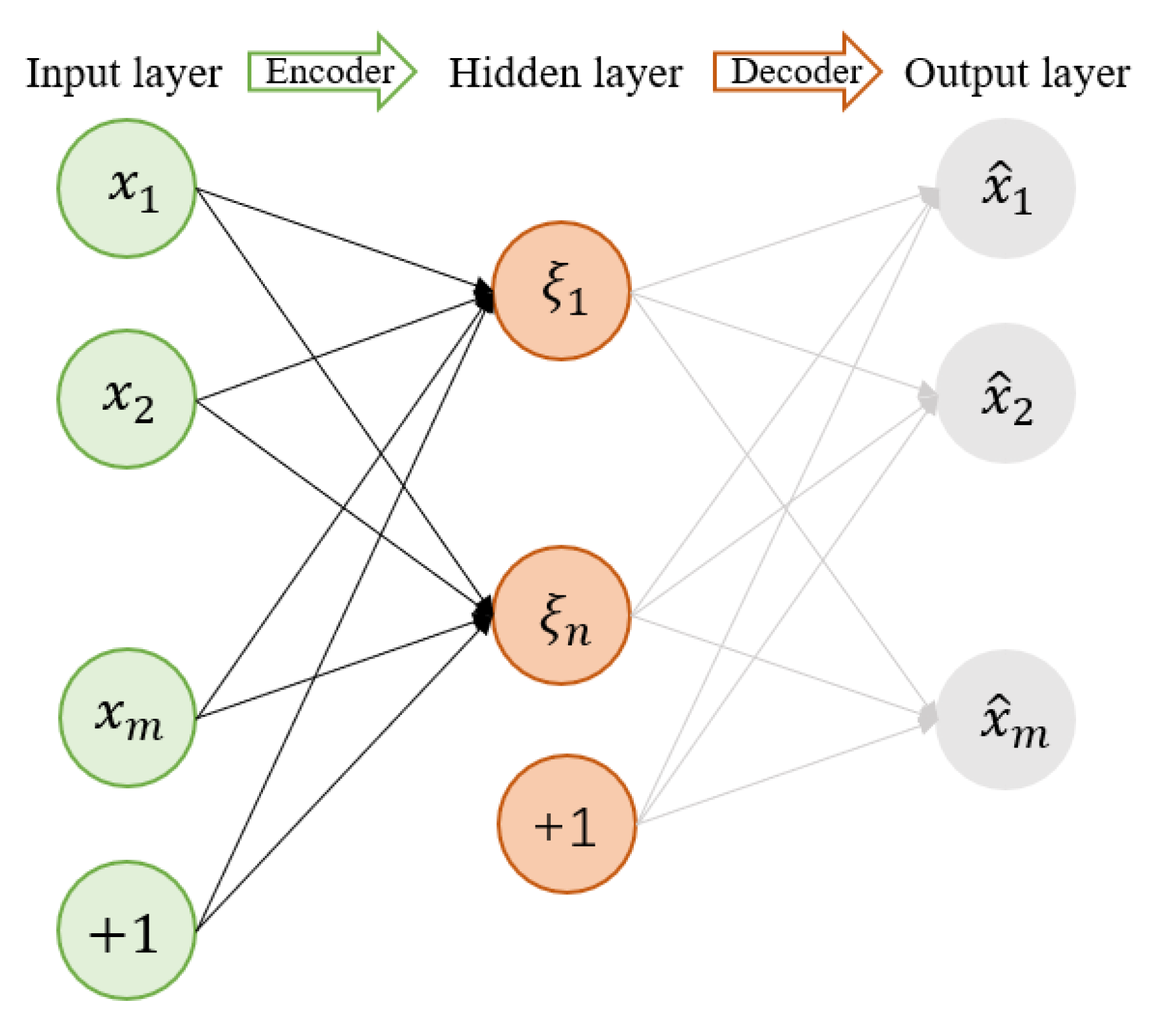
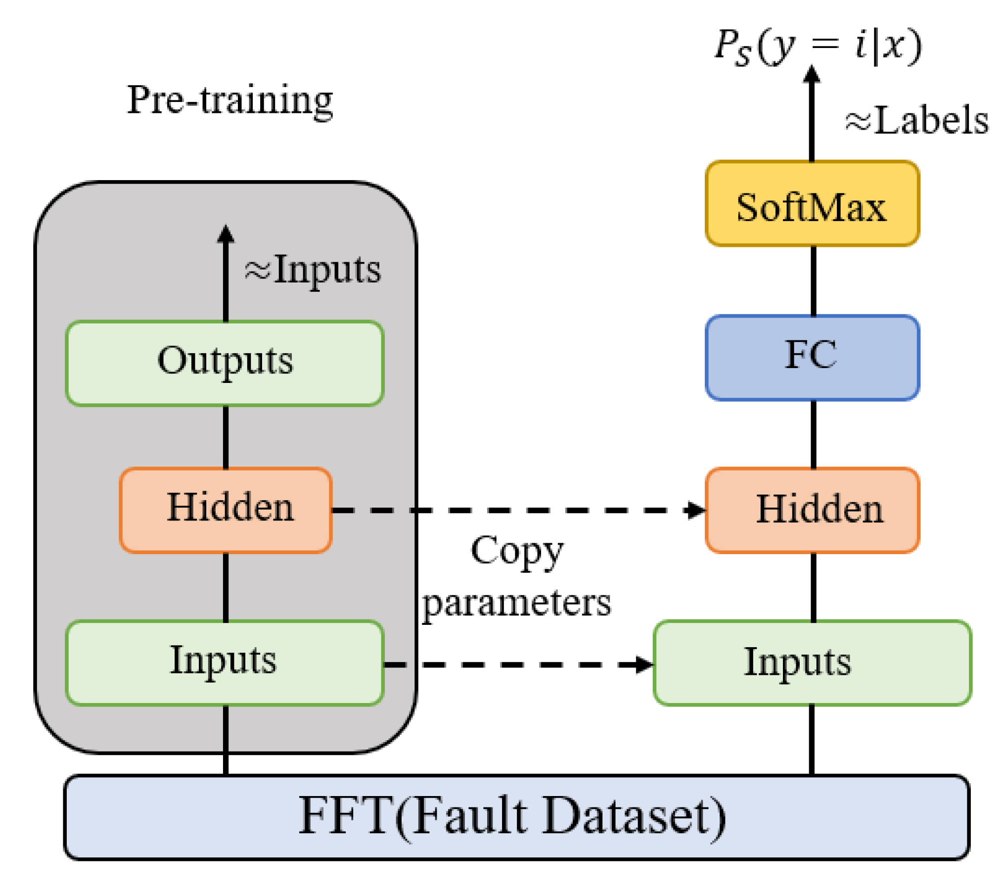
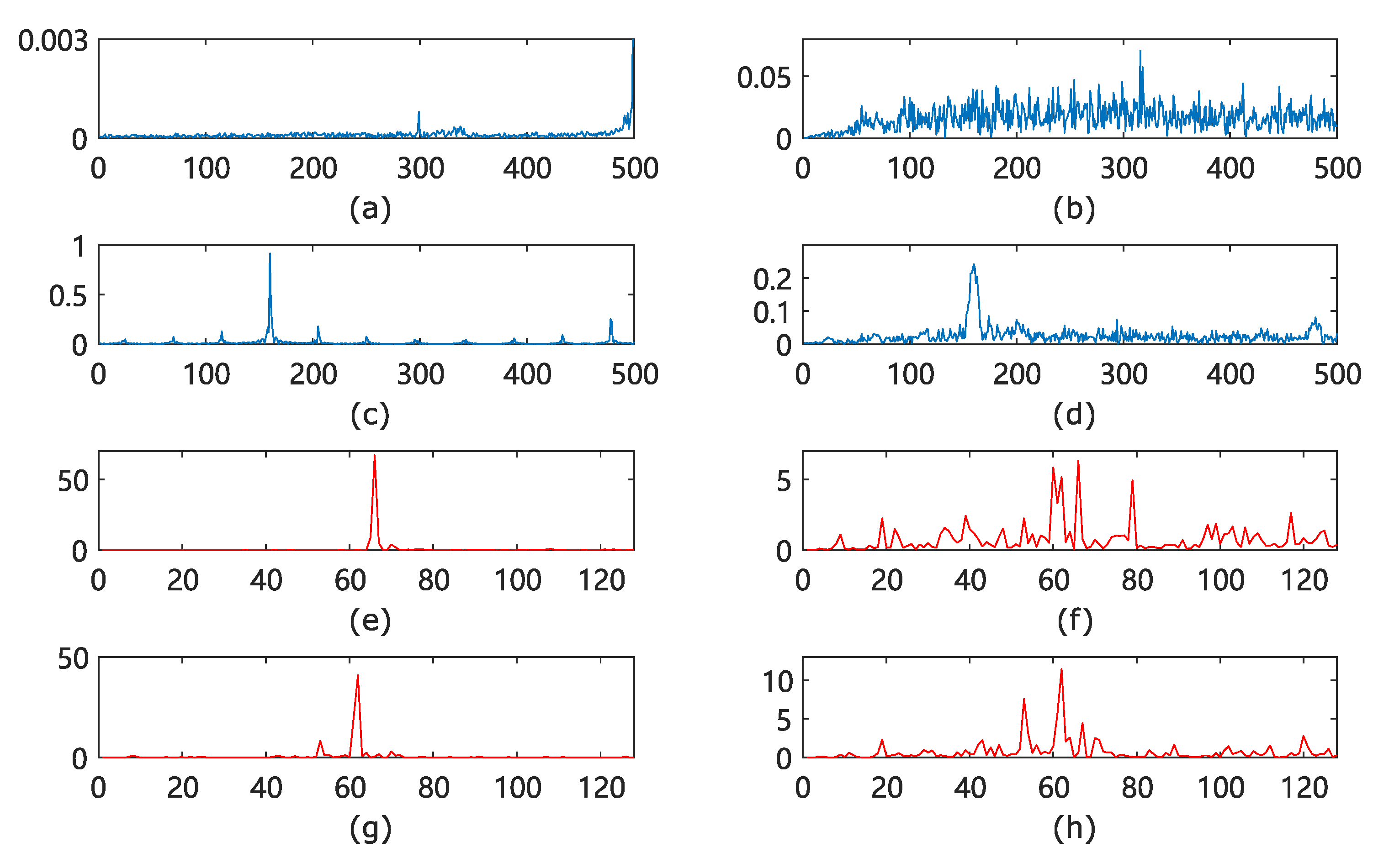
2.1. Sparse Auto Encoder Neural Network Based on Fast Fourier Transform
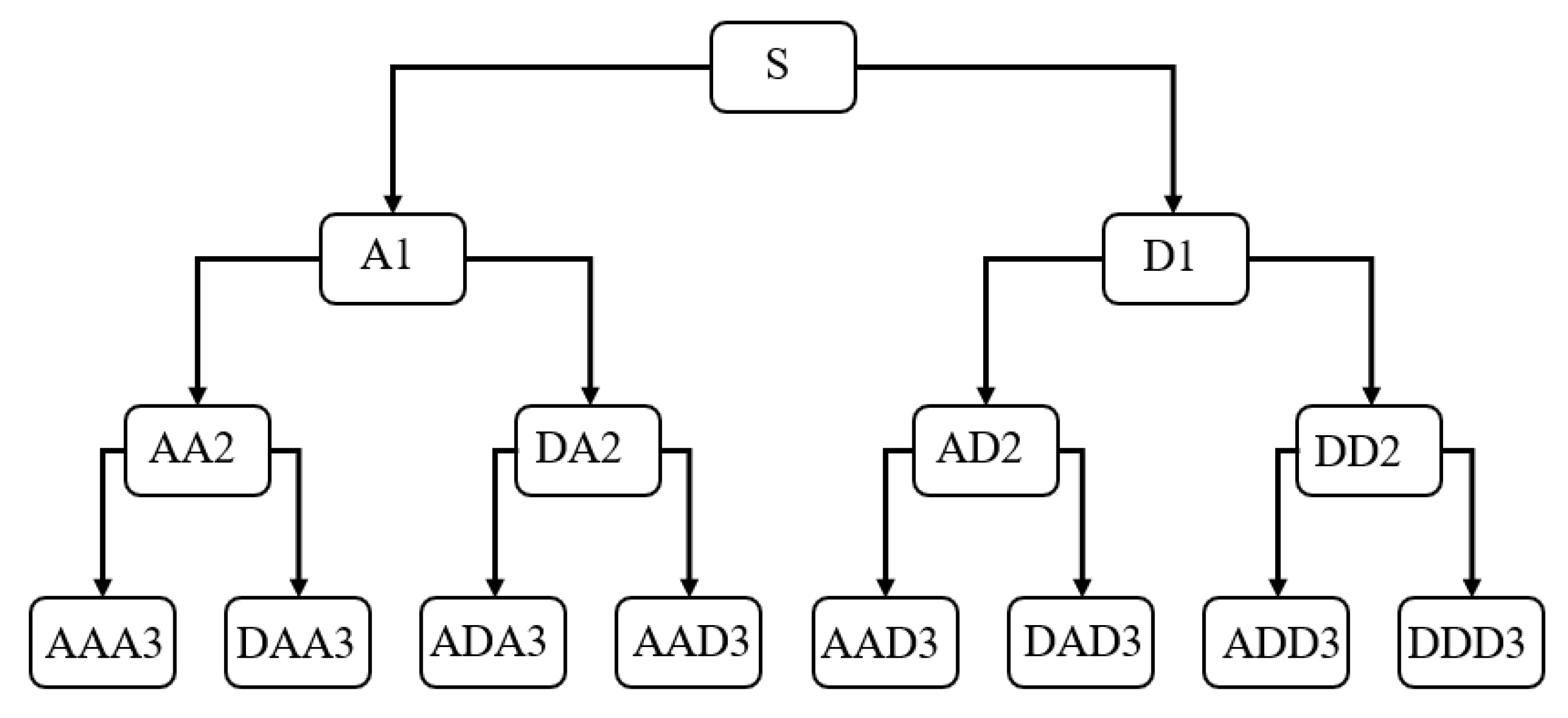
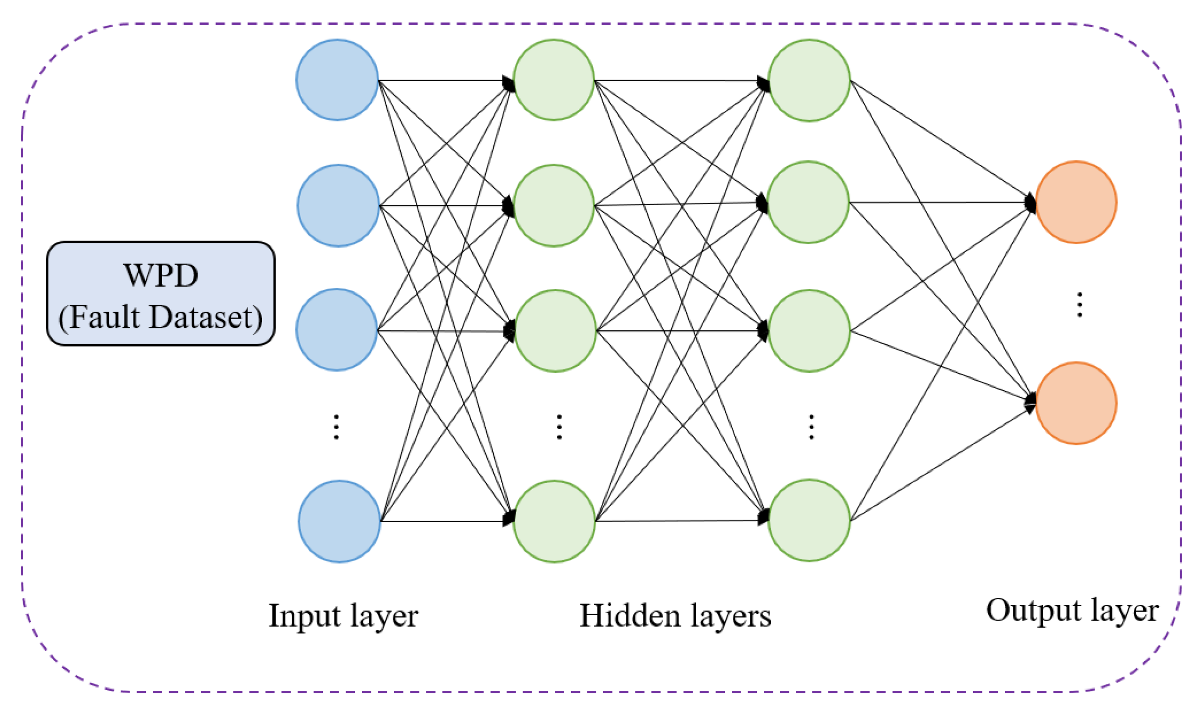
2.2. Neural Networks Based on Wavelet Packet Decomposition
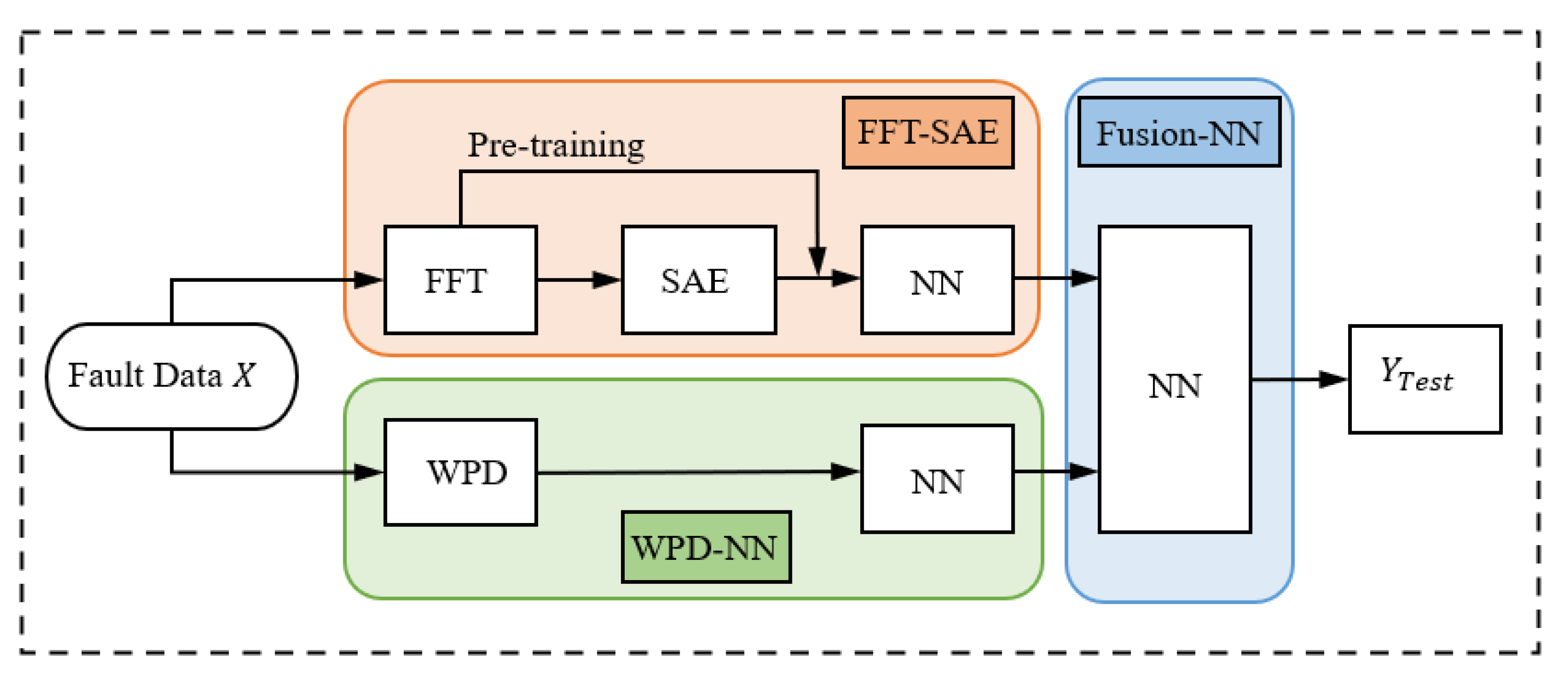
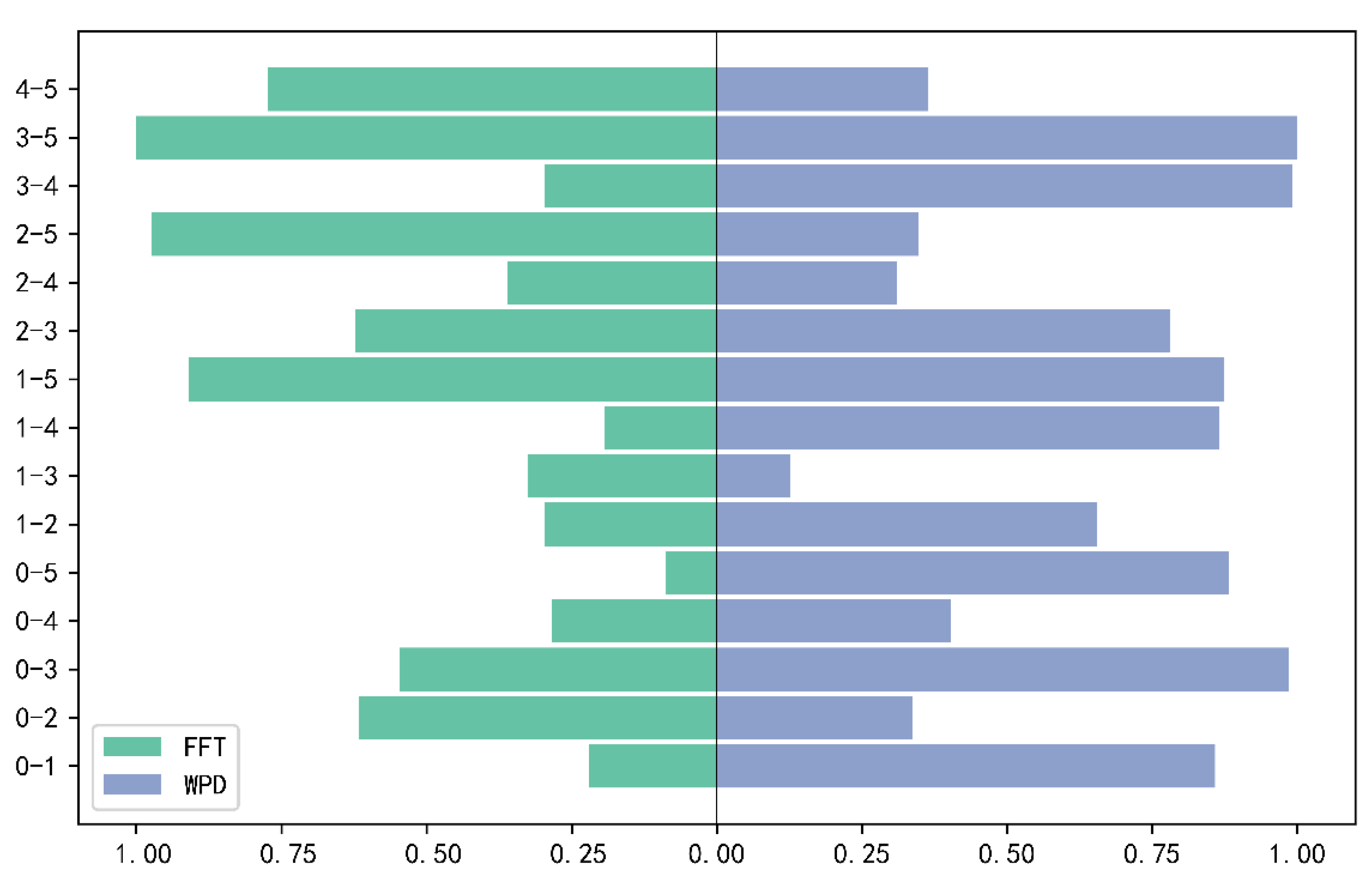
2.3. Fusion Fault Diagnosis Model
3. Results
3.1. Data Preparation
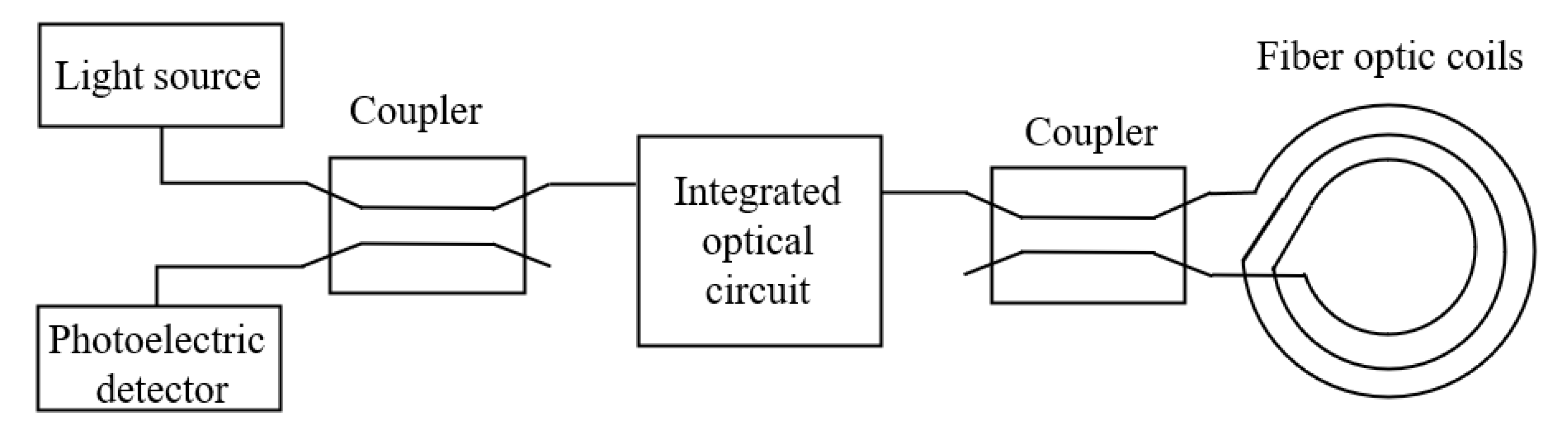
3.1.1. Mathematical Model of FOG
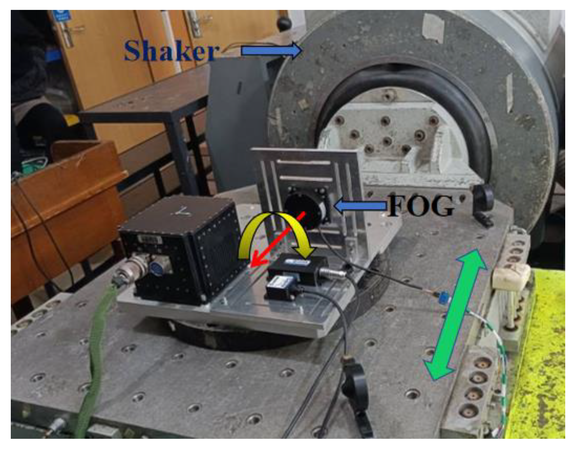
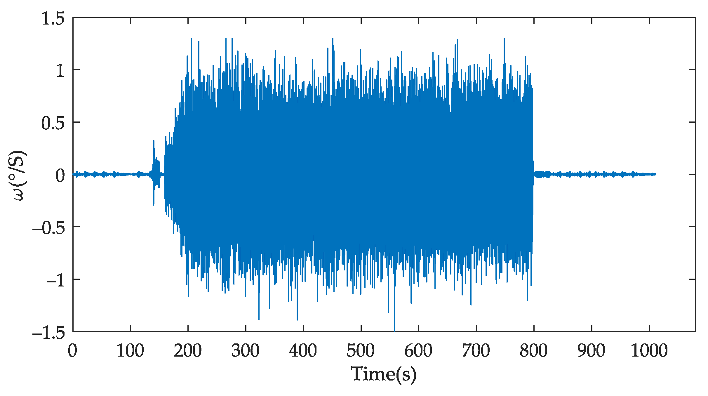
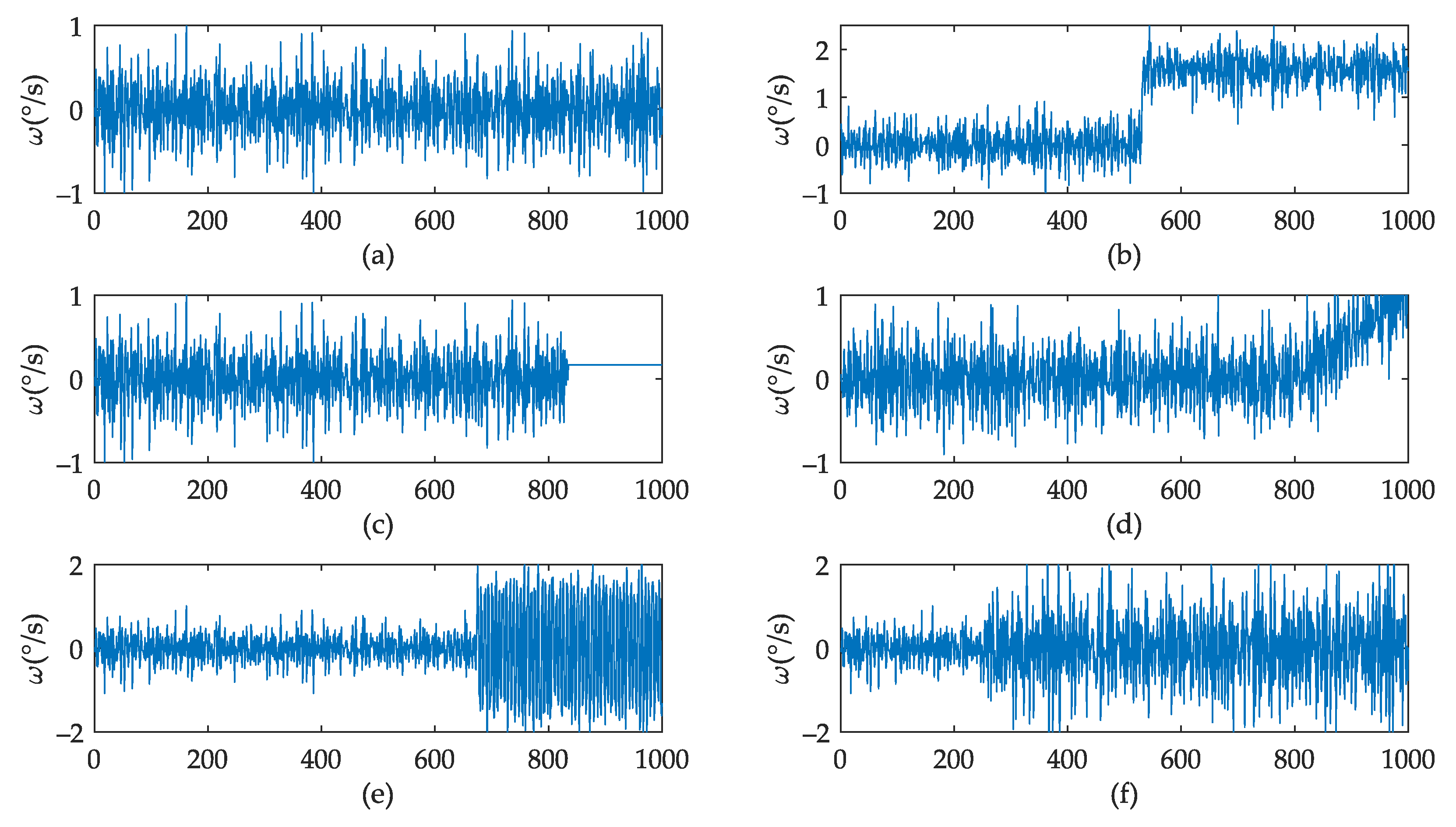
3.1.2. Generation of Fault Data
3.2. Experimental Results
3.2.1. Parameter Selection Experiment
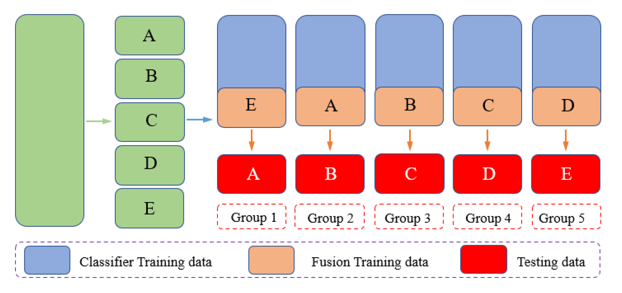
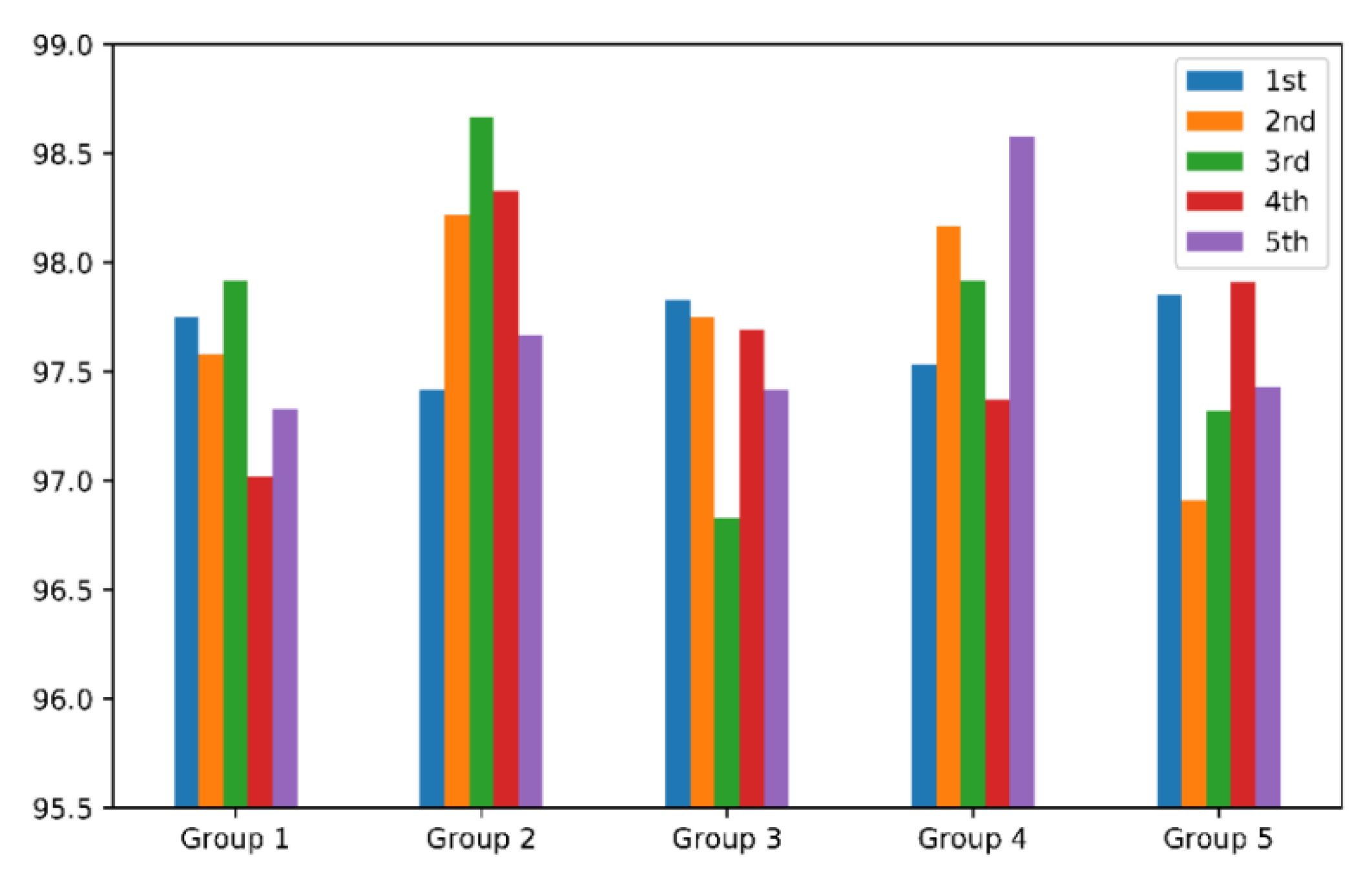
3.2.2. Stability Experiments of the Fusion Model
3.2.3. Comparisons with Other Methods
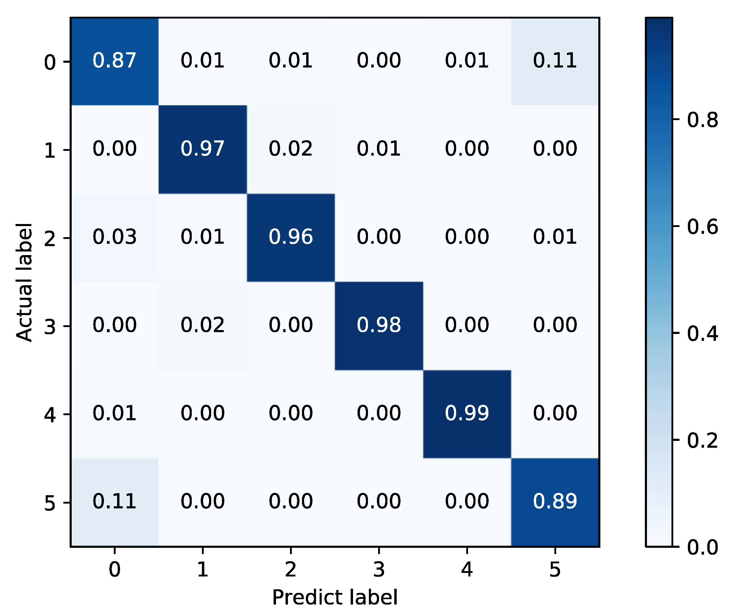
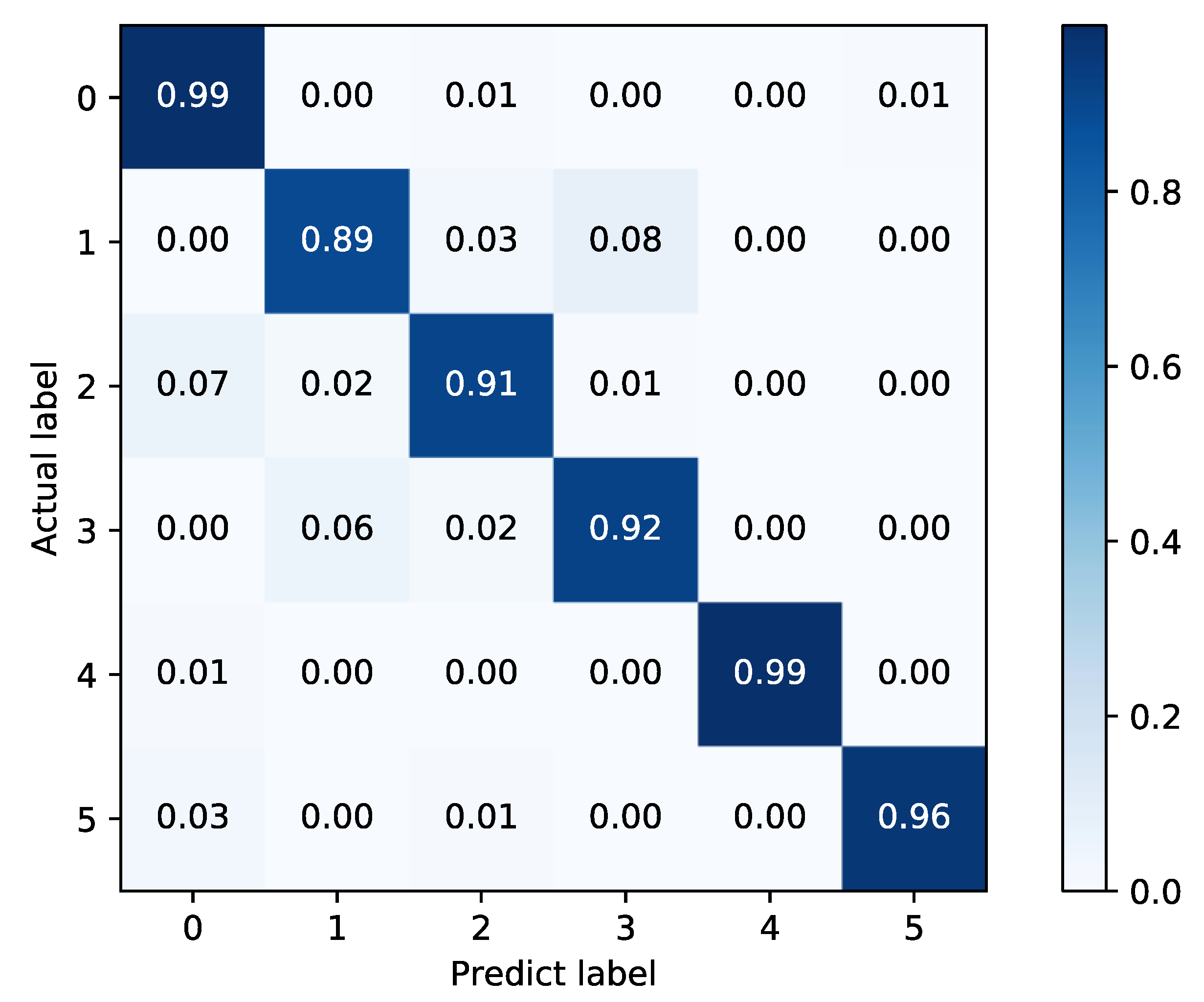
- Comparison with basic classifier.
- 2.
- Comparison with other methods.
4. Conclusions
Author Contributions
Funding
Institutional Review Board Statement
Informed Consent Statement
Data Availability Statement
Conflicts of Interest
Appendix A

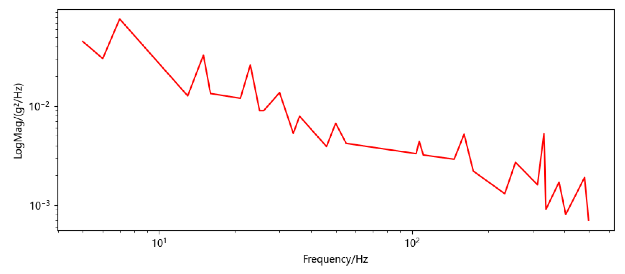
| Hz | g2/Hz | Hz | g2/Hz |
|---|---|---|---|
| 5 | 0.0451 | 104 | 0.0033 |
| 6 | 0.0303 | 107 | 0.0044 |
| 7 | 0.0761 | 111 | 0.0032 |
| 13 | 0.0127 | 147 | 0.0029 |
| 15 | 0.0327 | 161 | 0.0052 |
| 16 | 0.0134 | 175 | 0.0022 |
| 21 | 0.0120 | 233 | 0.0013 |
| 23 | 0.0261 | 257 | 0.0027 |
| 25 | 0.0090 | 314 | 0.0016 |
| 26 | 0.0090 | 333 | 0.0053 |
| 30 | 0.0137 | 339 | 0.0009 |
| 34 | 0.0053 | 382 | 0.0017 |
| 36 | 0.0079 | 406 | 0.0008 |
| 46 | 0.0039 | 482 | 0.0019 |
| 50 | 0.0067 | 500 | 0.0007 |
| 55 | 0.0042 | ||
| 1.29 grms | |||
Appendix B
| Section | Time to First Reuse (ms) | Time to Normal Use (ms) |
|---|---|---|
| WPD | 70.29 | 70.29 |
| FFT | 41.94 | 41.94 |
| SAE | 15.02 | 1.01 |
| NN | 6.96 | 0.99 |
| Fusion model | 6.98 | 0.99 |
| Total | 141.19 | 115.22 |
| Time offset | 1000.00 | |
References
- Gao, Z.; Cecati, C.; Ding, S.X. A Survey of Fault Diagnosis and Fault-Tolerant Techniques—Part I: Fault Diagnosis with Model-Based and Signal-Based Approaches. IEEE Trans. Ind. Electron. 2015, 62, 3757–3767. [Google Scholar] [CrossRef] [Green Version]
- Shao, H.; Jiang, H.; Lin, Y.; Li, X. A novel method for intelligent fault diagnosis of rolling bearings using ensemble deep auto-encoders. Mech. Syst. Signal Process. 2018, 102, 278–297. [Google Scholar] [CrossRef]
- Zuo, L.; Zhang, L.; Zhang, Z.-H.; Luo, X.-L.; Liu, Y. A spiking neural network-based approach to bearing fault diagnosis. J. Manuf. Syst. 2021, 61, 714–724. [Google Scholar] [CrossRef]
- Li, G.; Deng, C.; Wu, J.; Chen, Z.; Xu, X. Rolling Bearing Fault Diagnosis Based on Wavelet Packet Transform and Convolutional Neural Network. Appl. Sci. 2020, 10, 770. [Google Scholar] [CrossRef] [Green Version]
- Fernández-Francos, D.; Martínez-Rego, D.; Fontenla-Romero, O.; Alonso-Betanzos, A. Automatic bearing fault diagnosis based on one-class ν-SVM. Comput. Ind. Eng. 2013, 64, 357–365. [Google Scholar] [CrossRef]
- Li, H.; Hu, G.; Li, J.; Zhou, M. Intelligent fault diagnosis for large-scale rotating machines using binarized deep neural networks and random forests. IEEE Trans. Autom. Sci. Eng. 2021. [Google Scholar] [CrossRef]
- Chen, M.; Wu, J.; Wang, Y.; Jia, B.; Jiang, Y. Random forest based intelligent fault diagnosis for PV arrays using array voltage and string currents. Sensors 2018, 18, 1221. [Google Scholar] [CrossRef]
- Ahmad, Z.; Nguyen, T.-K.; Ahmad, S.; Nguyen, C.D.; Kim, J.-M. Multistage Centrifugal Pump Fault Diagnosis Using Informative Ratio Principal Component Analysis. Sensors 2022, 22, 179. [Google Scholar] [CrossRef]
- Nguyen, C.D.; Prosvirin, A.E.; Kim, C.H.; Kim, J.-M. Construction of a sensitive and speed invariant gearbox fault diagnosis model using an incorporated utilizing adaptive noise control and a stacked sparse autoencoder-based deep neural network. Sensors 2021, 21, 18. [Google Scholar] [CrossRef]
- Li, W.; Huang, R.; Li, J.; Liao, Y.; Chen, Z.; He, G.; Yan, R.; Gryllias, K. A perspective survey on deep transfer learning for fault diagnosis in industrial scenarios: Theories, applications and challenges. Mech. Syst. Signal Process. 2022, 167, 108487. [Google Scholar] [CrossRef]
- Wen, L.; Gao, L.; Li, X. A new deep transfer learning based on sparse auto-encoder for fault diagnosis. IEEE Trans. Syst. Man Cybern. Syst. 2019, 49, 136–144. [Google Scholar] [CrossRef]
- Han, Y.; Tang, B.; Deng, L. Multi-level wavelet packet fusion in dynamic ensemble convolutional neural network for fault diagnosis. Measurement 2018, 127, 246–255. [Google Scholar] [CrossRef]
- Tang, S.; Yuan, S.; Zhu, Y.; Li, G. An integrated deep learning method towards fault diagnosis of hydraulic axial piston pump. Sensors 2020, 20, 6576. [Google Scholar] [CrossRef]
- Zhang, X.; Wan, S.; He, Y.; Wang, X.; Dou, L. Teager energy spectral kurtosis of wavelet packet transform and its application in locating the sound source of fault bearing of belt conveyor. Measurement 2021, 173, 108367. [Google Scholar] [CrossRef]
- Sun, Y.; Cao, Y.; Li, P. Fault diagnosis for train plug door using weighted fractional wavelet packet decomposition energy entropy. Accid. Anal. Prev. 2022, 166, 106549. [Google Scholar] [CrossRef] [PubMed]
- Chinara, S. Automatic classification methods for detecting drowsiness using wavelet packet transform extracted time-domain features from single-channel EEG signal. J. Neurosci. Methods 2021, 347, 108927. [Google Scholar]
- Cai, J.; Wang, S.; Guo, W. Unsupervised embedded feature learning for deep clustering with stacked sparse auto-encoder. Expert Syst. Appl. 2021, 186, 115729. [Google Scholar] [CrossRef]
- Lei, Y. Clustering algorithm–based fault diagnosis. In Intelligent Fault Diagnosis and Remaining Useful Life Prediction of Rotating Machinery; Butterworth-Heinemann: Oxford, UK, 2017; pp. 175–229. [Google Scholar]
- Xiao, T. Research on Pose Measurement System of Shield Using the Combination of Inclinometer and Gyroscope. Master’s Thesis, Huazhong University of Science and Technology, Wuhan, China, 2013. [Google Scholar]
- Cai, H. Error Analysis and Compensation of Attitude Measurement System for TBM. Master’s Thesis, Huazhong University of Science and Technology, Wuhan, China, 2009. [Google Scholar]
- Yu, J.; Zhou, D.; He, P.; Huang, J. A new method for gyroscope fault diagnosis based on CGA RBFNN and multi-wavelet entropy. In Proceedings of the 2013 International Conference on Mechatronic Sciences, Electric Engineering and Computer (MEC), Shengyang, China, 20–22 December 2013; IEEE: New York, NY, USA, 2013; pp. 39–43. [Google Scholar]
- Liu, Q.; Cheng, J.; Guo, W. Research on Gyro Fault Diagnosis Method Based on Wavelet Packet Decomposition and Multi-class Least Squares Support Vector Machine. In Recent Trends in Intelligent Computing, Communication and Devices; Springer: Berlin/Heidelberg, Germany, 2020; pp. 789–797. [Google Scholar]
- Chen, X.; Xiao, M.; Sun, Y. Fiber optic gyro fault diagnosis based on improved sparrow search algorithm and support vector machine. J. Air Force Eng. Univ. Nat. Sci. Ed. 2021, 22, 33–40. [Google Scholar]
- Guan, J. Research on Fault Diagnosis Technology of Fiber Optic Gyro Based on Neural Network; Harbin Institute of Technology: Harbin, China, 2019. [Google Scholar]
- Song, H.; Hu, S.-L.; Zhou, K.-Y. Review on Development of Fault Diagnosis for Gyroscope. In Proceedings of the ITM Web of Conferences, Birmingham, UK, 2–4 May 2017; EDP Sciences: Les Ulis, France, 2017; p. 07001. [Google Scholar]
- Patton, R.J.; Uppal, F.J.; Simani, S.; Polle, B. Reliable fault diagnosis scheme for a spacecraft attitude control system. Proc. Inst. Mech. Eng. Part O J. Risk Reliab. 2008, 222, 139–152. [Google Scholar] [CrossRef]
- Chamoun, J.N.; Digonnet, M. Noise and Bias Error Due to Polarization Coupling in a Fiber Optic Gyroscope. J. Lightwave Technol. 2015, 33, 2839–2847. [Google Scholar] [CrossRef]
- Song, R.; Chen, X. Analysis of fiber optic gyroscope vibration error based on improved local mean decomposition and kernel principal component analysis. Appl. Opt. 2017, 56, 2265–2272. [Google Scholar] [CrossRef] [PubMed]
- Vincent, P.; Larochelle, H.; Lajoie, I.; Bengio, Y.; Manzagol, P.-A.; Bottou, L. Stacked denoising autoencoders: Learning useful representations in a deep network with a local denoising criterion. J. Mach. Learn. Res. 2010, 11, 3371–3408. [Google Scholar]
- Rifai, S.; Vincent, P.; Muller, X.; Glorot, X.; Bengio, Y. Contractive Auto-Encoders: Explicit Invariance during Feature Extraction; ICML: Broken Arrow, OK, USA, 2011. [Google Scholar]
- Zhang, K.; Zhang, J.; Ma, X.; Yao, C.; Zhang, L.; Yang, Y.; Wang, J.; Yao, J.; Zhao, H. History matching of naturally fractured reservoirs using a deep sparse autoencoder. SPE J. 2021, 26, 1700–1721. [Google Scholar] [CrossRef]
- Yang, Z.; Baraldi, P.; Zio, E. A method for fault detection in multi-component systems based on sparse autoencoder-based deep neural networks. Reliab. Eng. Syst. Saf. 2022, 220, 108278. [Google Scholar] [CrossRef]
- Ranzato, M.A.; Poultney, C.; Chopra, S.; Cun, Y. Efficient learning of sparse representations with an energy-based model. In Advances in Neural Information Processing Systems 19: Proceedings of the 2006 Conference; MIT Press: Cambridge, MA, USA, 2006; Volume 19. [Google Scholar]
- Mao, Z.; Xia, M.; Jiang, B.; Xu, D.; Shi, P. Incipient fault diagnosis for high-speed train traction systems via stacked generalization. IEEE Trans. Cybern. 2021. [Google Scholar] [CrossRef]
- Yuan, Z.; Song, N.; Pan, X. Fault diagnosis for space-borne fiber-optic gyroscopes using a hybrid method. IEEE Access 2020, 8, 194147. [Google Scholar] [CrossRef]
- Wu, W. Research on Fault Diagnosis Method for Gyroscope Based on Fuzzy Support Vector Machines. Master’s Thesis, Nanjing University of Aeronautics and Astronautics, Nanjing, China, 2016. [Google Scholar]
- Heredia, G.; Ollero, A.; Mahtani, R.; Bejar, M.; Musial, M. Detection of Sensor Faults in Autonomous Helicopters. In Proceedings of the IEEE International Conference on Robotics & Automation, Barcelona, Spain, 18–22 April 2006. [Google Scholar]

| Model | Structure (Units and Activation) | Hyperparameter | |
|---|---|---|---|
| FFT + SAE | Pre-training | Dense (1000, 128); activation = ‘Sigmoid’ Dense (128, 1000) | Max epochs = 10,000; Batchsize = 6000 |
| Beta = 0.01 | |||
| Optimizer = Adam (lr = 0.005) | |||
| Training | Dense (128, 64); activation = ‘Relu’ | Max epochs = 10,000; Batchsize = 3600 | |
| Dense (64, 32); activation = ‘Relu’ | Optimizer = Adam (lr = 0.005) | ||
| Dense (32, 6); activation = ‘SoftMax’ | Dropout rate 0.2 | ||
| WPD + NN | Dense (128, 64); activation = ‘Relu’ | Max epochs = 10,000; Batchsize = 3600 | |
| Dense (64, 32); activation = ‘Relu’ | Optimizer = Adam (lr = 0.005) | ||
| Dense (32, 6); activation = ‘SoftMax’ | Dropout rate 0.2 | ||
| Fusion model | Dense (12, 6); activation = ‘SoftMax’ | Max epochs = 10,000; Batchsize = 1200 | |
| Optimizer = Adam (lr = 0.005, weight decay = 0.0001) | |||
| Gyroscope Type: | FOGS107A |
|---|---|
| Zero bias stability: | <0.05°/h(10s,1σ) |
| Zero bias repeatability: | <0.05°/h(10s,1σ) |
| Random wandering factor: | <0.005°/√h |
| Dynamic measurement range: | ±500°/s |
| Output method: | RS422 |
| Ratio | WPD + NN | FFT + SAE | Fusion | std (%) |
|---|---|---|---|---|
| 4:4 | 93.19 | 91.94 | 96.65 | 0.48 |
| 5:3 | 94.03 | 93.30 | 97.27 | 0.55 |
| 5.5:2.5 | 94.52 | 93.37 | 97.42 | 0.49 |
| 6:2 | 94.51 | 94.50 | 97.93 | 0.58 |
| 7:1 | 94.85 | 94.44 | 97.17 | 0.66 |
| Method | Accuracy | Std. Deviation |
|---|---|---|
| WPD + NN | 95.62 | 0.29 |
| FFT + SAE | 94.14 | 0.34 |
| Fusion module | 97.93 | 0.58 |
Publisher’s Note: MDPI stays neutral with regard to jurisdictional claims in published maps and institutional affiliations. |
© 2022 by the authors. Licensee MDPI, Basel, Switzerland. This article is an open access article distributed under the terms and conditions of the Creative Commons Attribution (CC BY) license (https://creativecommons.org/licenses/by/4.0/).
Share and Cite
Zhang, W.; Zhang, D.; Zhang, P.; Han, L. A New Fusion Fault Diagnosis Method for Fiber Optic Gyroscopes. Sensors 2022, 22, 2877. https://doi.org/10.3390/s22082877
Zhang W, Zhang D, Zhang P, Han L. A New Fusion Fault Diagnosis Method for Fiber Optic Gyroscopes. Sensors. 2022; 22(8):2877. https://doi.org/10.3390/s22082877
Chicago/Turabian StyleZhang, Wanpeng, Dailin Zhang, Peng Zhang, and Lei Han. 2022. "A New Fusion Fault Diagnosis Method for Fiber Optic Gyroscopes" Sensors 22, no. 8: 2877. https://doi.org/10.3390/s22082877
APA StyleZhang, W., Zhang, D., Zhang, P., & Han, L. (2022). A New Fusion Fault Diagnosis Method for Fiber Optic Gyroscopes. Sensors, 22(8), 2877. https://doi.org/10.3390/s22082877