
An Extended Kalman Filter for Magnetic Field SLAM Using Gaussian Process Regression


Abstract
:1. Introduction
2. Modeling
2.1. Measurement Model
2.2. Dynamic Model
3. Ekf for Magnetic Field Slam
| Algorithm 1: EKF for magnetic field SLAM |
Input: Output: , , Initialisation: , , , (19) 1: for to N do 2: Dynamic update
3: Measurement update
4: Relinearization
5: end for |
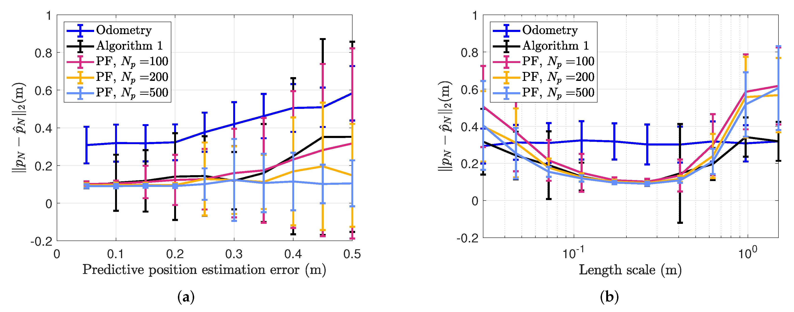
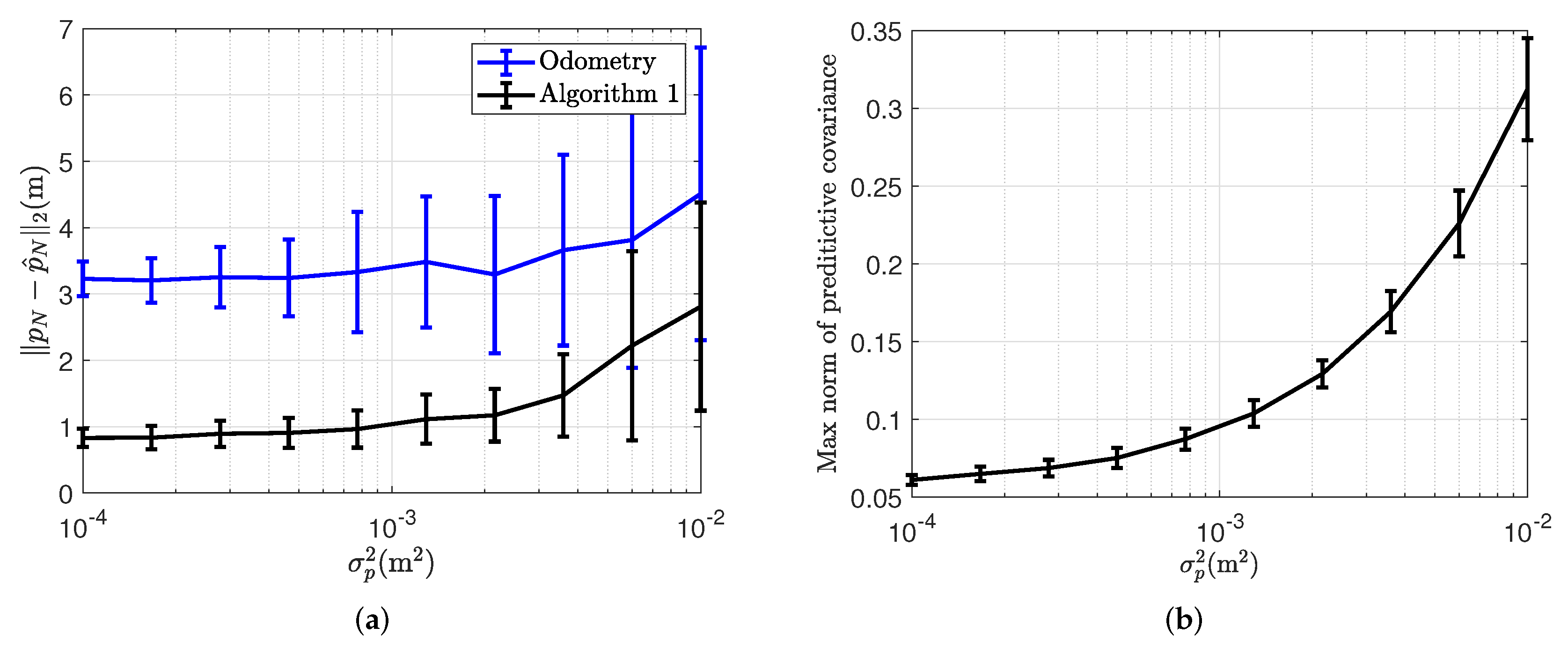
4. Simulations
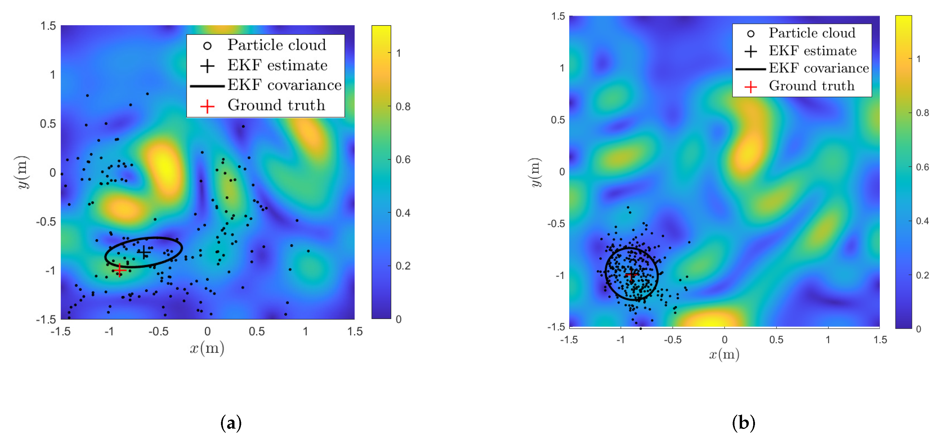
5. Experimental Results
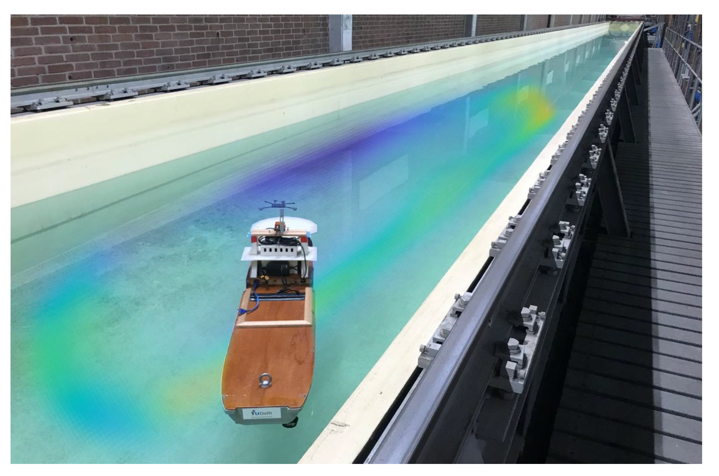
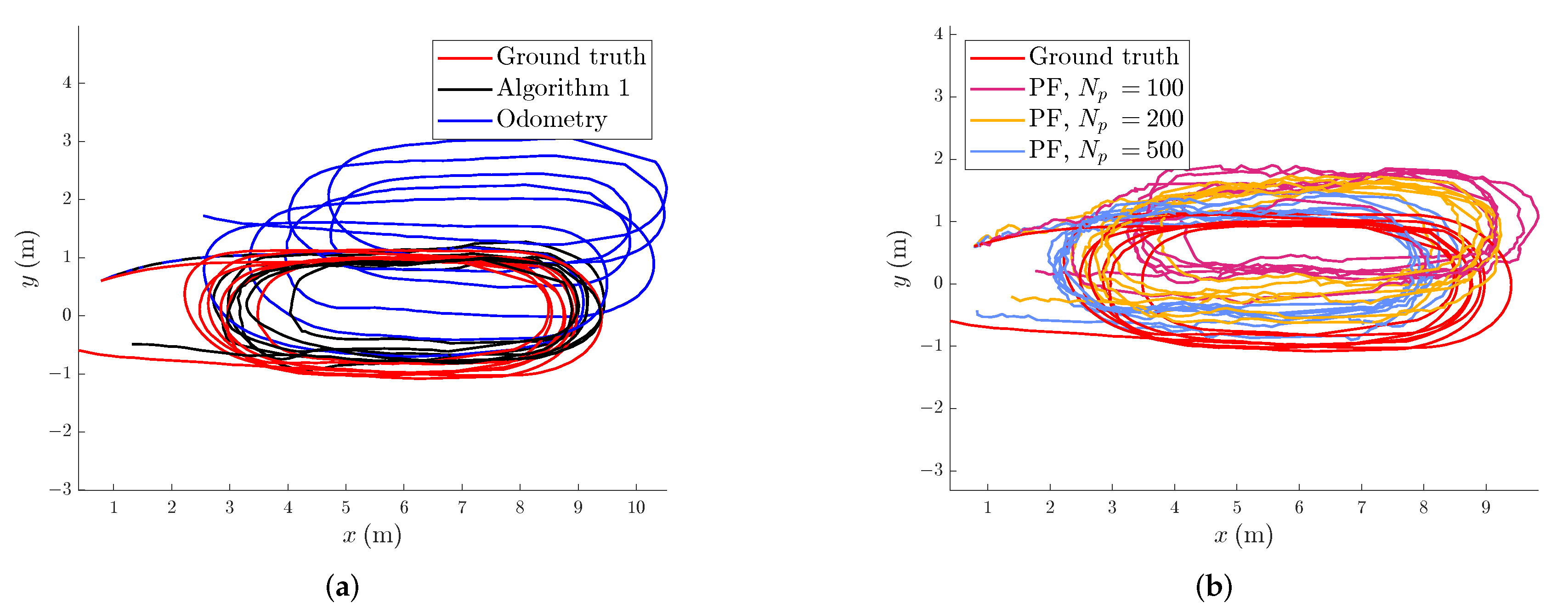
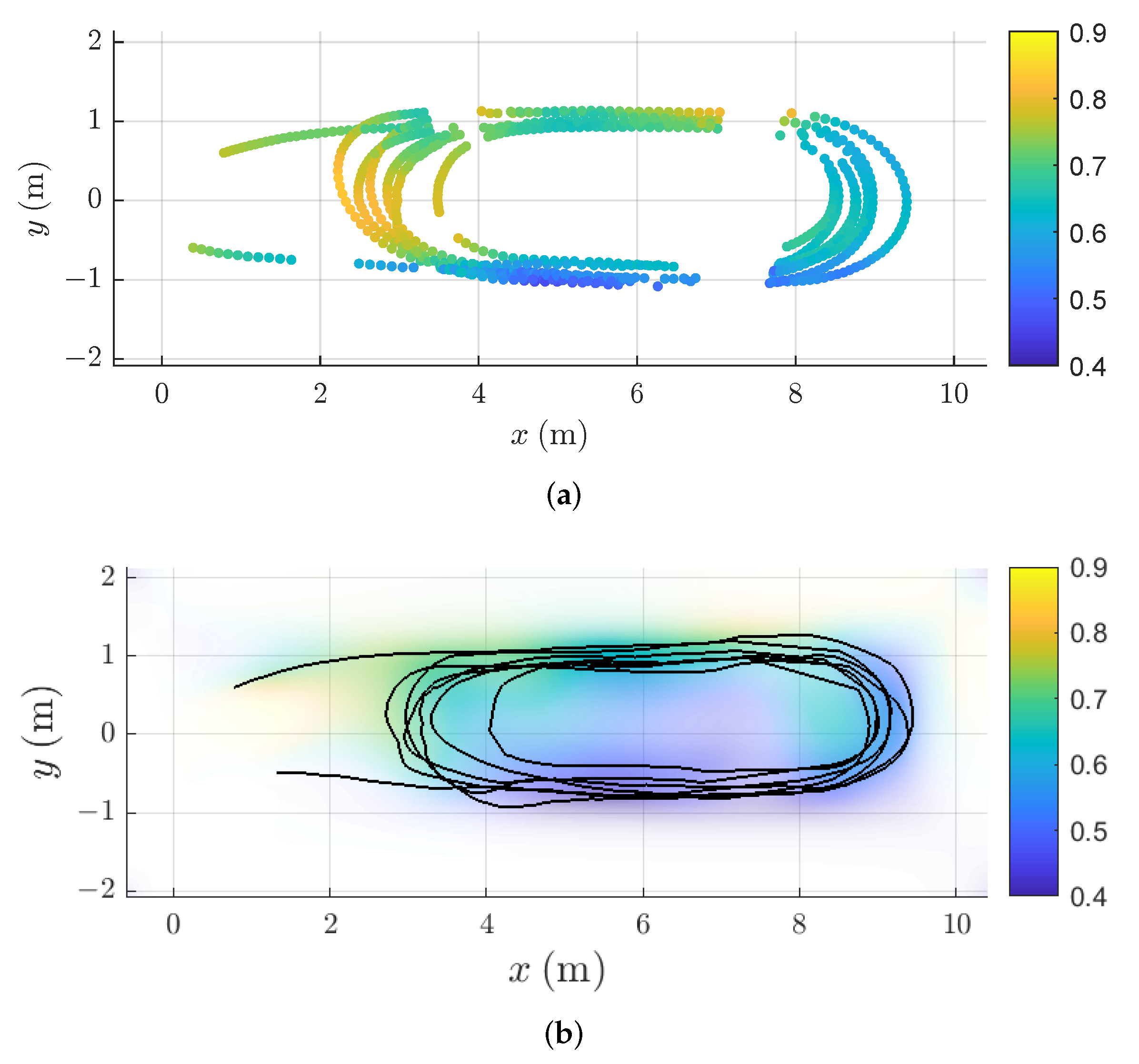
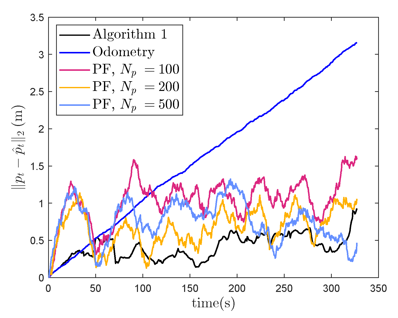
5.1. Model Ship Experiments
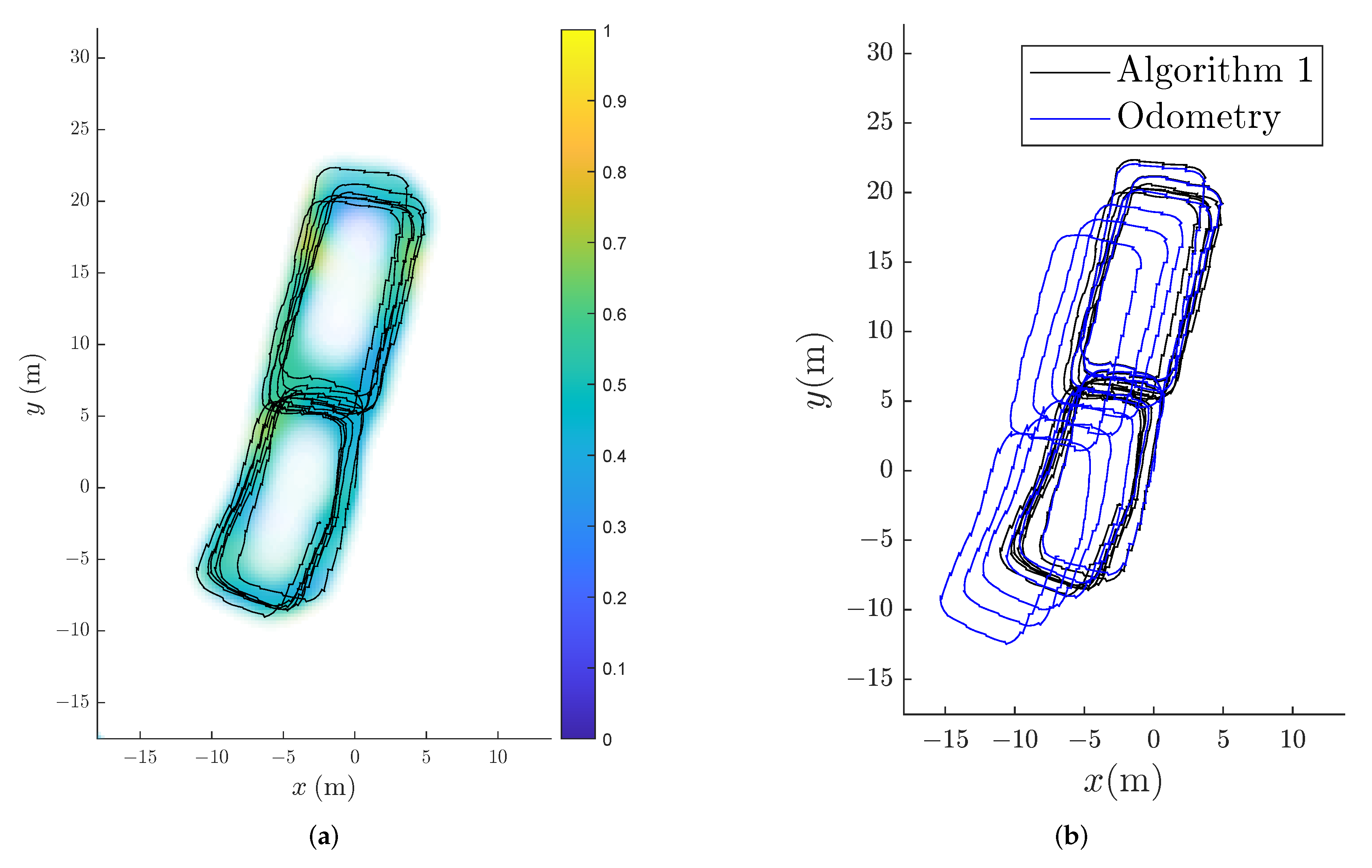
5.2. Magnetic Field Slam for Pedestrians with Foot-Mounted Sensor
6. Conclusions and Future Work
Author Contributions
Funding
Institutional Review Board Statement
Informed Consent Statement
Data Availability Statement
Acknowledgments
Conflicts of Interest
Abbreviations
| SLAM | Simultaneous localization and mapping |
| EKF | Extended Kalman filtering |
| RBPF | Rao-Blackwellized particle filter |
| GP | Gaussian process |
| IMU | Inertial measurement unit |
| ZUPT | Zero-velocity upate |
| RMSE | Root mean squared error |
| GNSS | Global navigation satelite system |
Appendix A. Analytical Jacobians
References
- Storms, W.; Shockley, J.; Raquet, J. Magnetic field navigation in an indoor environment. In Proceedings of the Ubiquitous Positioning Indoor Navigation and Location Based Service, Kirkkonummi, Finland, 14–15 October 2010; pp. 1–10. [Google Scholar]
- Paull, L.; Saeedi, S.; Seto, M.; Li, H. AUV Navigation and Localization: A Review. IEEE J. Ocean. Eng. 2014, 39, 131–149. [Google Scholar] [CrossRef]
- Dong, L.; Sun, D.; Han, G.; Li, X.; Hu, Q.; Shu, L. Velocity-Free Localization of Autonomous Driverless Vehicles in Underground Intelligent Mines. IEEE Trans. Veh. Technol. 2020, 69, 9292–9303. [Google Scholar] [CrossRef]
- Mekik, C.; Can, O. Multipath effects in RTK GPS and a case study. J. Aeronaut. Astronaut. Aviat. Ser. A 2010, 42, 231–240. [Google Scholar]
- Cadena, C.; Carlone, L.; Carrillo, H.; Latif, Y.; Scaramuzza, D.; Neira, J.; Reid, I.; Leonard, J.J. Past, Present, and Future of Simultaneous Localization and Mapping: Toward the Robust-Perception Age. IEEE Trans. Robot. 2016, 32, 1309–1332. [Google Scholar] [CrossRef] [Green Version]
- Woodman, O.J. An Introduction to Inertial Navigation; Technical Report; Computer laboratory University of Cambridge: Cambridge, UK, 2007. [Google Scholar]
- Solin, A.; Kok, M.; Wahlström, N.; Schön, T.B.; Särkkä, S. Modeling and Interpolation of the Ambient Magnetic Field by Gaussian Processes. IEEE Trans. Robot. 2018, 34, 1112–1127. [Google Scholar] [CrossRef] [Green Version]
- Kok, M.; Solin, A. Scalable Magnetic Field SLAM in 3D Using Gaussian Process Maps. In Proceedings of the 21st International Conference on Information Fusion, Cambridge, UK, 10–13 July 2018; pp. 1353–1360. [Google Scholar] [CrossRef] [Green Version]
- Yamazaki, K.; Kato, K.; Ono, K.; Saegusa, H.; Tokunaga, K.; Iida, Y.; Yamamoto, S.; Ashiho, K.; Fujiwara, K.; Takahashi, N. Analysis of magnetic disturbance due to buildings. IEEE Trans. Magn. 2003, 39, 3226–3228. [Google Scholar] [CrossRef]
- Haverinen, J.; Kemppainen, A. A global self-localization technique utilizing local anomalies of the ambient magnetic field. In Proceedings of the IEEE International Conference on Robotics and Automation, Kobe, Japan, 12–17 May 2009; pp. 3142–3147. [Google Scholar] [CrossRef]
- Vallivaara, I.; Haverinen, J.; Kemppainen, A.; Röning, J. Simultaneous localization and mapping using ambient magnetic field. In Proceedings of the IEEE International Conference on Multisensor Fusion and Integration for Intelligent Systems (MFI), Karlsruhe, Germany, 23–25 September 2010; pp. 14–19. [Google Scholar] [CrossRef]
- Kemppainen, A.; Haverinen, J.; Vallivaara, I.; Röning, J. Near-optimal SLAM exploration in Gaussian processes. In Proceedings of the IEEE Conference on Multisensor Fusion and Integration, Salt Lake City, UT, USA, 5–7 September 2010; pp. 7–13. [Google Scholar] [CrossRef]
- Vallivaara, I.; Haverinen, J.; Kemppainen, A.; Röning, J. Magnetic field-based SLAM method for solving the localization problem in mobile robot floor-cleaning task. In Proceedings of the IEEE 15th International Conference on Advanced Robotics: New Boundaries for Robotics (ICAR 2011), Tallinn, Estonia, 20–23 June 2011; pp. 198–203. [Google Scholar] [CrossRef]
- Chung, J.; Donahoe, M.; Schmandt, C.; Kim, I.J.; Razavi, P.; Wiseman, M. Indoor location sensing using geo-magnetism. In Proceedings of the 9th International Conference on Mobile Systems, Applications, and Services, Bethesda, MA, USA, 28 June–1 July 2011; pp. 141–154. [Google Scholar] [CrossRef] [Green Version]
- Le Grand, E.; Thrun, S. 3-Axis magnetic field mapping and fusion for indoor localization. In Proceedings of the IEEE International Conference on Multisensor Fusion and Integration for Intelligent Systems (MFI), Hamburg, Germany, 13–15 September 2012; pp. 358–364. [Google Scholar] [CrossRef]
- Kim, S.E.; Kim, Y.; Yoon, J.; Kim, E.S. Indoor positioning system using geomagnetic anomalies for smartphones. In Proceedings of the International Conference on Indoor Positioning and Indoor Navigation (IPIN), Sydney, NSW, Australia, 13–15 November 2012; pp. 1–5. [Google Scholar]
- Frassl, M.; Angermann, M.; Lichtenstern, M.; Robertson, P.; Julian, B.J.; Doniec, M. Magnetic maps of indoor environments for precise localization of legged and non-legged locomotion. In Proceedings of the IEEE/RSJ International Conference on Intelligent Robots and Systems, Tokyo, Japan, 3–7 November 2013; pp. 913–920. [Google Scholar] [CrossRef] [Green Version]
- Robertson, P.; Frassl, M.; Angermann, M.; Doniec, M.; Julian, B.; Puyol, M.; Khider, M.; Lichtenstern, M.; Bruno, L. Simultaneous Localization and Mapping for Pedestrians using Distortions of the Local Magnetic Field Intensity in Large Indoor Environments. In Proceedings of the International Conference on Indoor Positioning and Indoor Navigation (IPIN 2013), Montbeliard, France, 28–31 October 2013. [Google Scholar] [CrossRef]
- Jung, J.; Lee, S.M.; Myung, H. Indoor Mobile Robot Localization and Mapping Based on Ambient Magnetic Fields and Aiding Radio Sources. IEEE Trans. Instrum. Meas. 2015, 64, 1922–1934. [Google Scholar] [CrossRef]
- Solin, A.; Särkkä, S.; Kannala, J.; Rahtu, E. Terrain navigation in the magnetic landscape: Particle filtering for indoor positioning. In Proceedings of the European Navigation Conference (ENC), Helsinki, Finland, 30 May–2 June 2016; pp. 1–9. [Google Scholar] [CrossRef]
- Kim, H.S.; Seo, W.; Baek, K. Indoor Positioning System Using Magnetic Field Map Navigation and an Encoder System. Sensors 2017, 17, 651. [Google Scholar] [CrossRef]
- Viset, F.; Gravdahl, J.; Kok, M. Magnetic field norm SLAM using Gaussian process regression in foot-mounted sensors. In Proceedings of the European Control Conference, Delft, The Netherlands, 29 June–2 July 2021; pp. 392–398. [Google Scholar] [CrossRef]
- Zheng, H.; Wang, H.; Wu, L.; Chai, H.; Wang, Y. Simulation research on gravity-geomagnetism combined aided underwater navigation. J. Navig. 2013, 66, 83–98. [Google Scholar] [CrossRef] [Green Version]
- Nygren, I. Robust and efficient terrain navigation of underwater vehicles. In Proceedings of the IEEE/ION Position, Location and Navigation Symposium, Monterey, CA, USA, 5–8 May 2008; pp. 923–932. [Google Scholar] [CrossRef]
- Lager, M.; Topp, E.A.; Malec, J. Underwater Terrain Navigation Using Standard Sea Charts and Magnetic Field Maps. In Proceedings of the IEEE International Conference on Multisensor Fusion and Integration for Intelligent Systems (MFI), Daegu, Korea, 16–18 November 2017; pp. 78–84. [Google Scholar] [CrossRef]
- Tal, A.; Klein, I.; Katz, R. Inertial Navigation System/Doppler Velocity Log (INS/DVL) Fusion with Partial DVL Measurements. Sensors 2017, 17, 415. [Google Scholar] [CrossRef]
- Tyrén, C. Magnetic terrain navigation. In Proceedings of the 5th International Symposium on Unmanned Untethered Submersible Technology (UUST 1987), Durham, NH, USA, June 1987; pp. 245–256. [Google Scholar] [CrossRef]
- Wu, Z.; Hu, X.; Wu, M.; Mu, H.; Cao, J.; Zhang, K.; Tuo, Z. An experimental evaluation of autonomous underwater vehicle localization on geomagnetic map. Appl. Phys. Lett. 2013, 103, 104102. [Google Scholar] [CrossRef]
- Wu, Y.; Shi, W. On Calibration of Three-Axis Magnetometer. IEEE Sens. J. 2015, 15, 6424–6431. [Google Scholar] [CrossRef] [Green Version]
- Huang, Y.; Hao, Y. Method of separating dipole magnetic anomaly from geomagnetic field and application in underwater vehicle localization. In Proceedings of the IEEE International Conference on Information and Automation, Harbin, China, 20–23 June 2010; pp. 1357–1362. [Google Scholar] [CrossRef]
- Teixeira, F.C.; Quintas, J.; Pascoal, A. Robust methods of magnetic navigation of marine robotic vehicles. IFAC-PapersOnLine 2017, 50, 3470–3475. [Google Scholar] [CrossRef]
- Mu, H.; Wu, M.; Hu, X.; Hongxu, M. Geomagnetic surface navigation using adaptive EKF. In Proceedings of the Second IEEE Conference on Industrial Electronics and Applications, Harbin, China, 23–25 May 2007; pp. 2821–2825. [Google Scholar] [CrossRef]
- Canciani, A.; Raquet, J. Airborne Magnetic Anomaly Navigation. IEEE Trans. Aerosp. Electron. Syst. 2017, 53, 67–80. [Google Scholar] [CrossRef]
- Quintas, J.; Cruz, J.; Pascoal, A.; Teixeira, F.C. A Comparison of Nonlinear Filters for Underwater Geomagnetic Navigation. In Proceedings of the IEEE/OES Autonomous Underwater Vehicles Symposium (AUV), St. Johns, NL, Canada, 30 September–2 October 2020; pp. 1–6. [Google Scholar] [CrossRef]
- Liu, S.; Mingas, G.; Bouganis, C.S. Parallel resampling for particle filters on FPGAs. In Proceedings of the International Conference on Field-Programmable Technology (FPT), Shanghai, China, 10–12 December 2014; pp. 191–198. [Google Scholar] [CrossRef]
- Varsi, A.; Maskell, S.; Spirakis, P.G. An O(log2N) Fully-Balanced Resampling Algorithm for Particle Filters on Distributed Memory Architectures. Algorithms 2021, 14, 342. [Google Scholar] [CrossRef]
- Solin, A.; Särkkä, S. Hilbert Space Methods for Reduced-Rank Gaussian Process Regression. Stat. Comput. 2020, 30, 419–446. [Google Scholar] [CrossRef] [Green Version]
- Kok, M.; Schön, T.B. Magnetometer Calibration Using Inertial Sensors. IEEE Sens. J. 2016, 16, 5679–5689. [Google Scholar] [CrossRef] [Green Version]
- Wahlström, N.; Gustafsson, F. Magnetometer Modeling and Validation for Tracking Metallic Targets. IEEE Trans. Signal Process. 2014, 62, 545–556. [Google Scholar] [CrossRef] [Green Version]
- Skog, I. OpenShoe Matlab Framework. In OpenShoe—Foot-Mounted INS for Every Foot; KTH Royal Institute of Technology, Stockholm, Sweden and Indian Institute of Science: Bangalore, India, 2011; Available online: http://www.openshoe.org/?page_id=362 (accessed on 18 November 2021).
- Kok, M.; Hol, J.D.; Schön, T.B. Using Inertial Sensors for Position and Orientation Estimation. Found. Trends Signal Process. 2017, 11, 1–153. [Google Scholar] [CrossRef] [Green Version]
- Wahlström, N.; Kok, M.; Schön, T.B.; Gustafsson, F. Modeling magnetic fields using Gaussian processes. In Proceedings of the IEEE International Conference on Acoustics, Speech and Signal Processing, Vancouver, BC, Canada, 26–31 May 2013; pp. 3522–3526. [Google Scholar] [CrossRef] [Green Version]
- Chen, Z. Bayesian Filtering: From Kalman Filters to Particle Filters, and Beyond. Statistics 2003, 182, 1–69. [Google Scholar] [CrossRef]
- Gustafsson, F. Statistical Sensor Fusion; Studentlitteratur AB: Lund, Sweden, 2013. [Google Scholar]
- Arulampalam, M.; Maskell, S.; Gordon, N.; Clapp, T. A tutorial on particle filters for online nonlinear/non-Gaussian Bayesian tracking. IEEE Trans. Signal Process. 2002, 50, 174–188. [Google Scholar] [CrossRef] [Green Version]
- Foxlin, E. Pedestrian tracking with shoe-mounted inertial sensors. IEEE Comput. Graph. Appl. 2005, 25, 38–46. [Google Scholar] [CrossRef] [PubMed]
- Nilsson, J.; Skog, I.; Händel, P.; Hari, K.V.S. Foot-mounted INS for everybody—An open-source embedded implementation. In Proceedings of the IEEE/ION Position, Location and Navigation Symposium, Myrtle Beach, SC, USA, 23–26 April 2012; pp. 140–145. [Google Scholar] [CrossRef] [Green Version]
- Skoglund, M.A.; Hendeby, G.; Axehill, D. Extended Kalman filter modifications based on an optimization view point. In Proceedings of the 18th International Conference on Information Fusion (Fusion), Washington, DC, USA, 6–9 July 2015; pp. 1856–1861. [Google Scholar]


| Trajectory RMSEs | Data Set 1 | Data Set 2 | Data Set 3 | Data Set 4 |
|---|---|---|---|---|
| Algorithm 1 | 0.53 ± 0.15 | 0.58 ± 0.18 | 0.53 ± 0.24 | 0.98 ± 0.62 |
| RBPF with 100 particles | 0.85 ± 0.27 | 0.92 ± 0.26 | 0.95 ± 0.42 | 1.53 ± 0.53 |
| RBPF with 200 particles | 0.85 ± 0.22 | 0.89 ± 0.27 | 0.98 ± 0.47 | 1.48 ± 0.46 |
| RBPF with 500 particles | 0.87 ± 0.19 | 0.86 ± 0.24 | 1.00 ± 0.40 | 1.53 ± 0.50 |
| Odometry | 1.98 ± 0.54 | 1.52 ± 0.48 | 1.76 ± 0.52 | 1.65 ± 0.47 |
| Runtimes | Data Set 1 | Data Set 2 | Data Set 3 | Data Set 4 |
|---|---|---|---|---|
| Algorithm 1 | 0.06 ± 0.01 | 0.05 ± 0.00 | 0.14 ± 0.01 | 0.05 ± 0.00 |
| RBPF with 100 particles | 12.85 ± 0.26 | 9.24 ± 0.10 | 21.55 ± 0.32 | 9.91 ± 0.14 |
| RBPF with 200 particles | 25.70 ± 0.49 | 18.44 ± 0.166 | 42.64 ± 0.27 | 19.72 ± 0.20 |
| RBPF with 500 particles | 64.24 ± 0.82 | 46.02 ± 0.20 | 106.93 ± 0.34 | 49.43 ± 1.29 |
Publisher’s Note: MDPI stays neutral with regard to jurisdictional claims in published maps and institutional affiliations. |
© 2022 by the authors. Licensee MDPI, Basel, Switzerland. This article is an open access article distributed under the terms and conditions of the Creative Commons Attribution (CC BY) license (https://creativecommons.org/licenses/by/4.0/).
Share and Cite
Viset, F.; Helmons, R.; Kok, M. An Extended Kalman Filter for Magnetic Field SLAM Using Gaussian Process Regression. Sensors 2022, 22, 2833. https://doi.org/10.3390/s22082833
Viset F, Helmons R, Kok M. An Extended Kalman Filter for Magnetic Field SLAM Using Gaussian Process Regression. Sensors. 2022; 22(8):2833. https://doi.org/10.3390/s22082833
Chicago/Turabian StyleViset, Frida, Rudy Helmons, and Manon Kok. 2022. "An Extended Kalman Filter for Magnetic Field SLAM Using Gaussian Process Regression" Sensors 22, no. 8: 2833. https://doi.org/10.3390/s22082833
APA StyleViset, F., Helmons, R., & Kok, M. (2022). An Extended Kalman Filter for Magnetic Field SLAM Using Gaussian Process Regression. Sensors, 22(8), 2833. https://doi.org/10.3390/s22082833