
Deep Learning-Based Indoor Localization Using Multi-View BLE Signal

 ,
,  , , , ,
Abstract
:1. Introduction
- ML-powered BLE-based indoor positioning via multiple anchor AoA estimation using both raw IQ values and RSSI estimates is proposed for the first time;
- A range of novel deep learning architectures, including fully connected multilayer perceptrons and CNNs are proposed and studied regarding their pros and cons;
- Joint anchor AoA estimates allowing distributed processing across the anchors is studied, to the best of our knowledge, for the first time. In particular, tuples of APs are grouped in smaller models that are then combined to produce the final prediction. Thus, hardware for a single computational expensive unit is replaced by less computationally demanding units distributed among the APs, facilitating embedded implementations;
- It is shown that deep learning methods yield robust indoor localization generalization, given environmental changes, e.g., different LOS-blocking obstacles and altered AP arrangements. To the best of our knowledge, no other study for indoor localization based on machine learning evaluates the generalizability of its models in different environments than the ones used in training;
- A data augmentation strategy is introduced that allows for reducing the training data size with minimal impact on performance. The performance improvement potential of joint anchor estimates vs. single anchors is also studied;
- A novel high spatial resolution dataset with multiple furniture configurations produced with realistic ray-tracing simulations is provided in open access mode.
2. Materials and Methods
2.1. Theoretical Foundation
2.2. System Setup and Data Preprocessing
2.3. NN Model Architectures
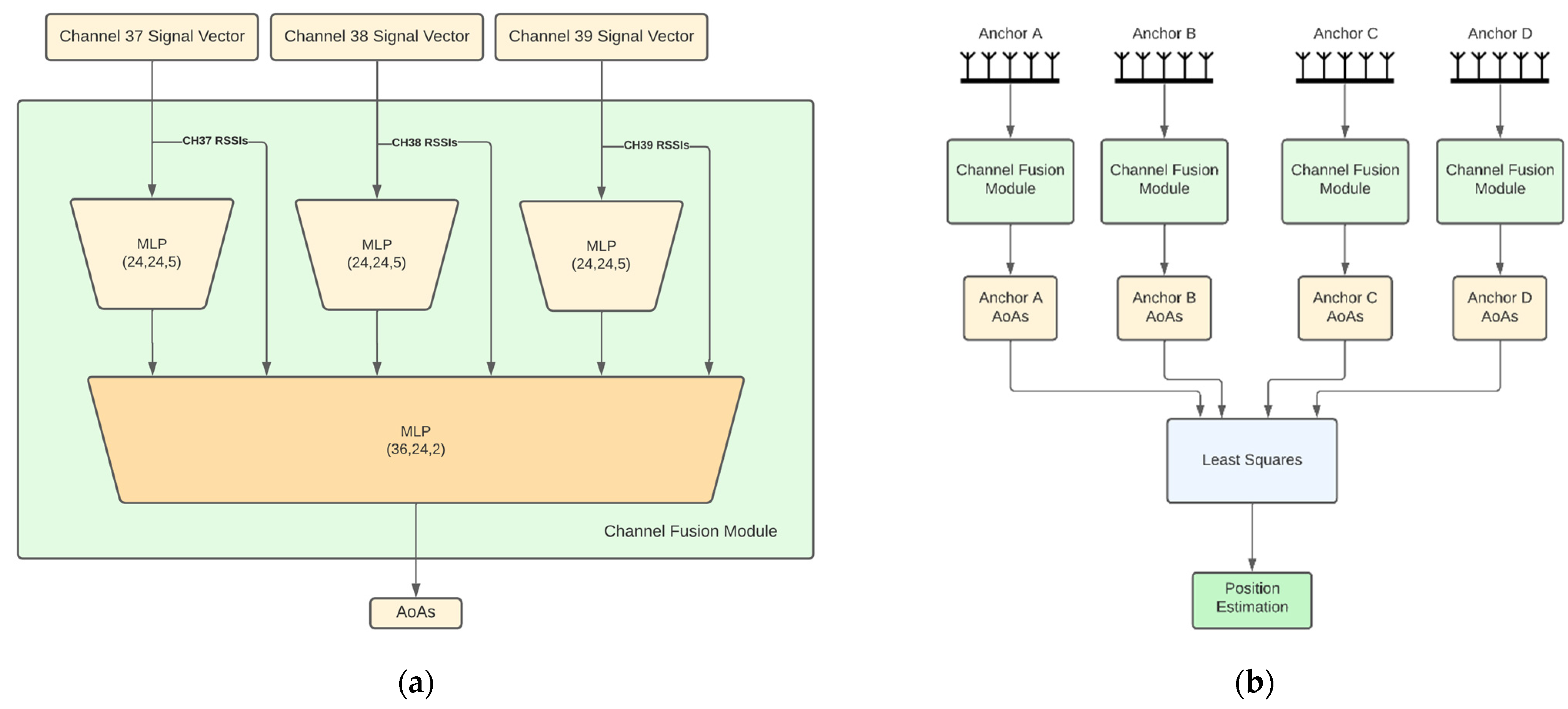
- Independent APs: In this architecture (Figure 1b), each AP has its own model for AoA estimates and the models are trained independently from each other. Each AP model input consists of three feature vectors of length 10, one per channel. Each vector consists of 9 IQ values and the channel RSSI value. This vector is hereafter referred to as channel signal vector. Each channel signal vector is fed to a different 3-layer neural network that produces a 5-dimensional latent representation. The 3 latent representations are then concatenated together with the RSSIs and fed to a 3-layer channel fusion MLP, which outputs the 2 angular directions (azimuth and elevation) of the AoA. In the sequel, we refer to this module as the channel fusion module (Figure 1a). Note that this architecture along with the ones presented later on, are directly extendable to more than 3 BLE channels and are not bound to the configuration that is chosen here for demonstration purposes. An advantage of the independent APs architecture is that the computational requirements are distributed across the anchors. However, this architecture does not exploit the fact that the APs are placed in fixed positions in a specific room, so the signal received by an AP from a tag placed anywhere in the room also conveys information about the AoA of this signal to the rest of the APs. This shortcoming is addressed by joint AP architectures discussed next.
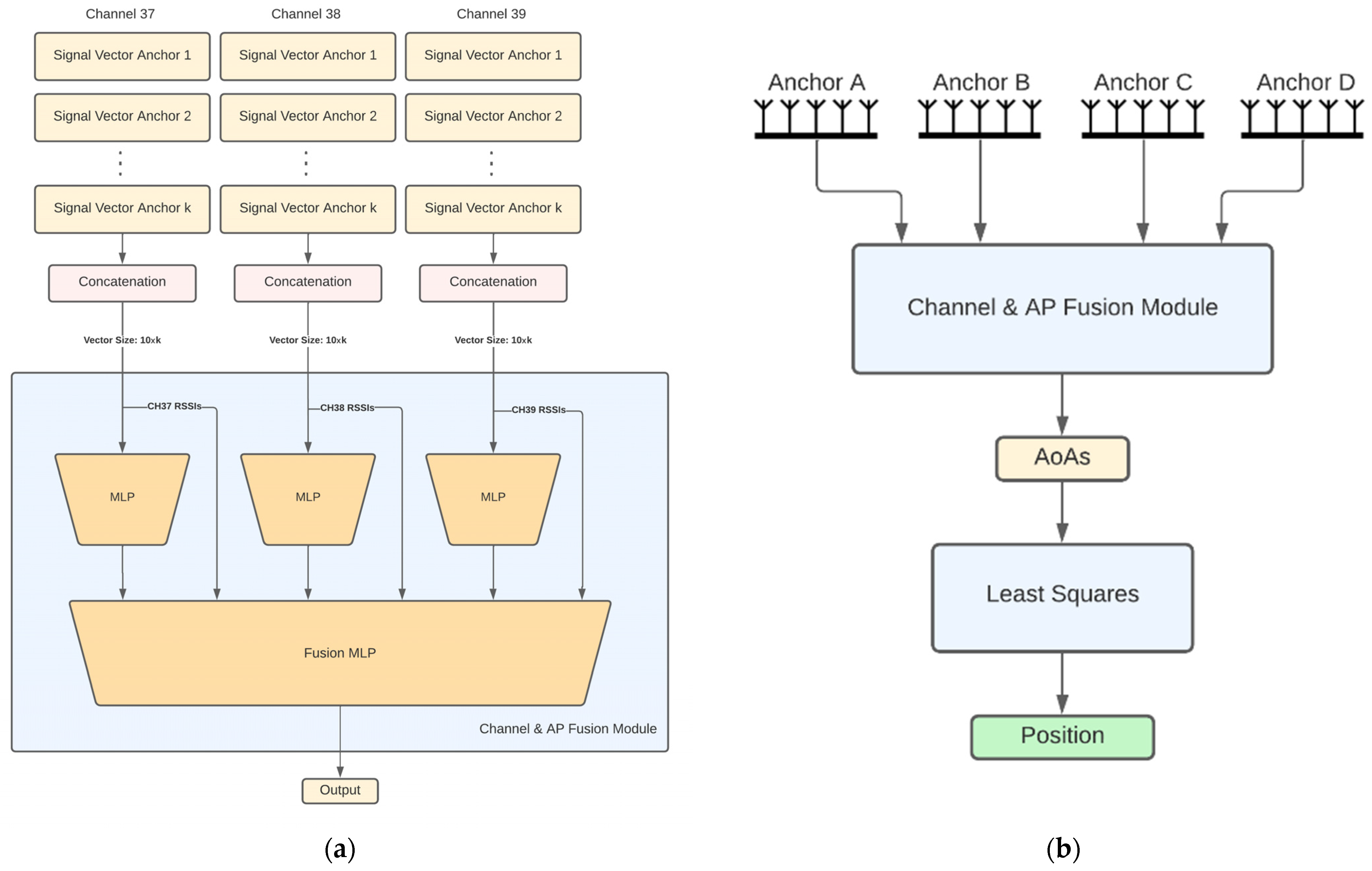
- Fully joint APs: This architecture aims to jointly estimate the AoA values of all APs using the respective received signals. Before going into the details for this architecture, let us first describe the channel and AP fusion module shown in Figure 2a, which is the main building block of this architecture and the following ones. This NN module first computes a latent representation for each channel and for a set of APs of size k, where k is a hyperparameter. To this end, the channel signal vectors of all anchors are concatenated per channel and fed as input to 3 different 3-layer MLPs with layer sizes 60, 40 and 12. Then the outputs of these MLPs are concatenated and, together with all the channel RSSIs, are fed into another 2-layer fusion MLP with layers of size 64 and 8, respectively. The fully joint AP architecture, shown in Figure 2b, is essentially the channel and AP fusion module. Accordingly, the fusion MLP output layer has 8 nodes to produce the final AoA estimates for all APs (2 angular directions per AoA × 4 APs). An advantage of this architecture compared to the independent AP one is the performance improvement, as will also be discussed in Section 3. A disadvantage is the lack of the distributed processing capability, which means that a powerful enough central computing unit is required to collect all signals and run the model.
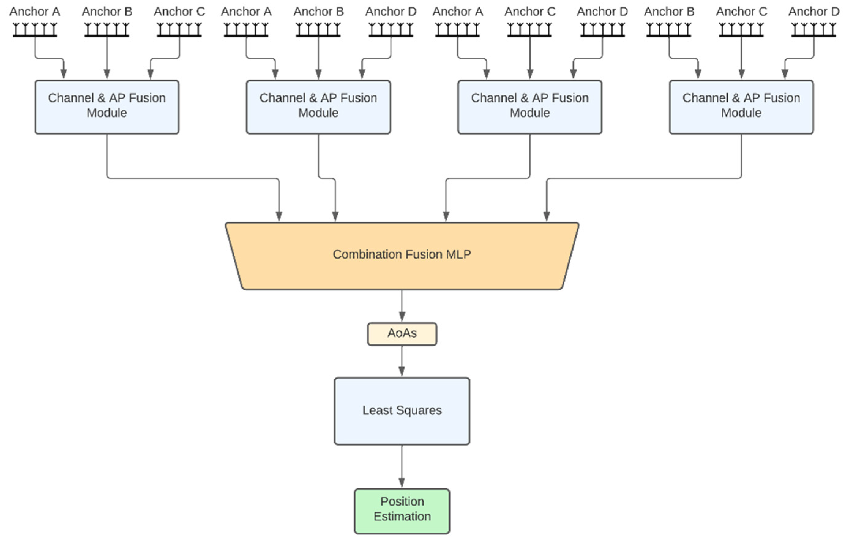
- Tuples of APs: This architecture aims to combine the best features of the two aforementioned architectures, namely, high performance and distributed computing potential. The idea is to jointly tackle k-combinations with repetition. Taking for example k = 3, exemplary possible AP combinations are ABC, ABD, ACD and BCD. Then, the corresponding triplets of APs architecture is shown in Figure 3, where the channel signal vectors of the four distinct triplets feed corresponding channel and AP fusion modules. In this case the three different MLPs of the channel and AP fusion module consist of 2-layers with sizes 24 and 9 and the Fusion MLP consists of 2-layers as well, but this time with sizes 27 and 12. Subsequently, the latent representations from the outputs of these models are concatenated and fed to a final 3-layer combination fusion MLP, with sizes 32, 16 and 8. The final output are the 8 AoA values for all 4 APs. As shown in Section 3, the performance of this architecture is similar, if not better, to that of the fully joint setup. In addition, the computational complexity can be distributed across the four APs if edge computing units embedded in the APs perform the computations of each channel and AP fusion module in parallel. The computations for the MLP that performs the final fusion along with the LS-based estimates of the positioning, still need to be performed subsequently. Similar to the triplets of APs architecture, one can also define the pairs of APs architecture.
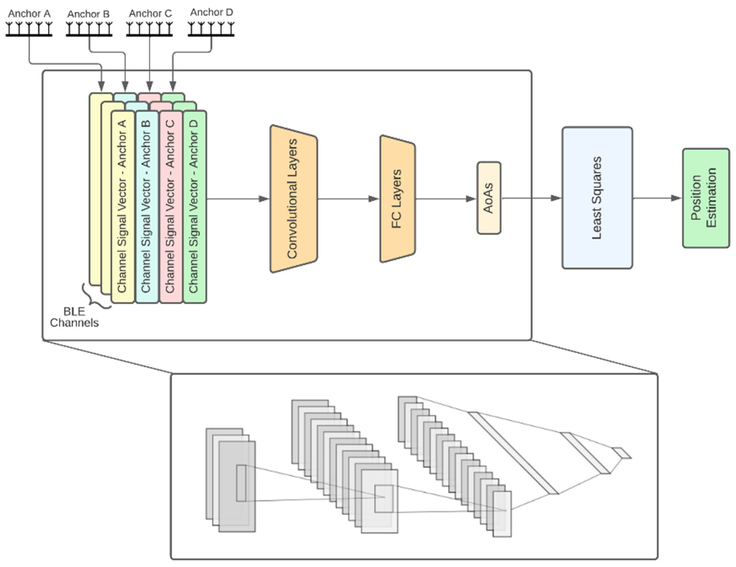
- CNN-based joint APs: This is an alternative joint architecture that operates on measurements taken from all four APs simultaneously using convolutional neural networks (CNNs), as shown in Figure 4. A major difference compared to the architecture of fully joint APs is that the channel and APs fusion module has been replaced by convolutional layers. To achieve this, the channel signal vectors are rearranged to form a 2D image-like representation of size 10 × 4 × 3, where the dimensions correspond to the APs, the channel signal vectors and the BLE channels, respectively. The 2 convolutional layers use kernels of size 4 × 1 and 3 × 2, respectively, and are followed by 3 fully connected layers, as shown in Figure 4.
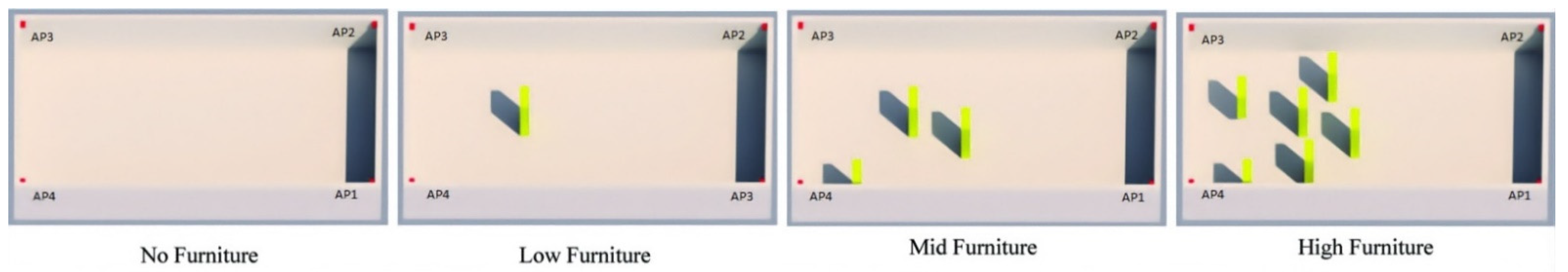
2.4. Simulation Environment
- The no LoS-blocking furniture case (referred to as “No Furniture”);
- Having one piece of LoS-blocking furniture, covering 0.5% of the room’s area (referred to as “Low Furniture”);
- Having three pieces of LoS-blocking furniture, covering 1.5% of the room’s area (referred to as “Mid Furniture”);
- Having six pieces of LoS-blocking furniture, covering 3% of the room’s area (referred to as “High Furniture”).
3. Results
3.1. Performance on a Fixed Environment
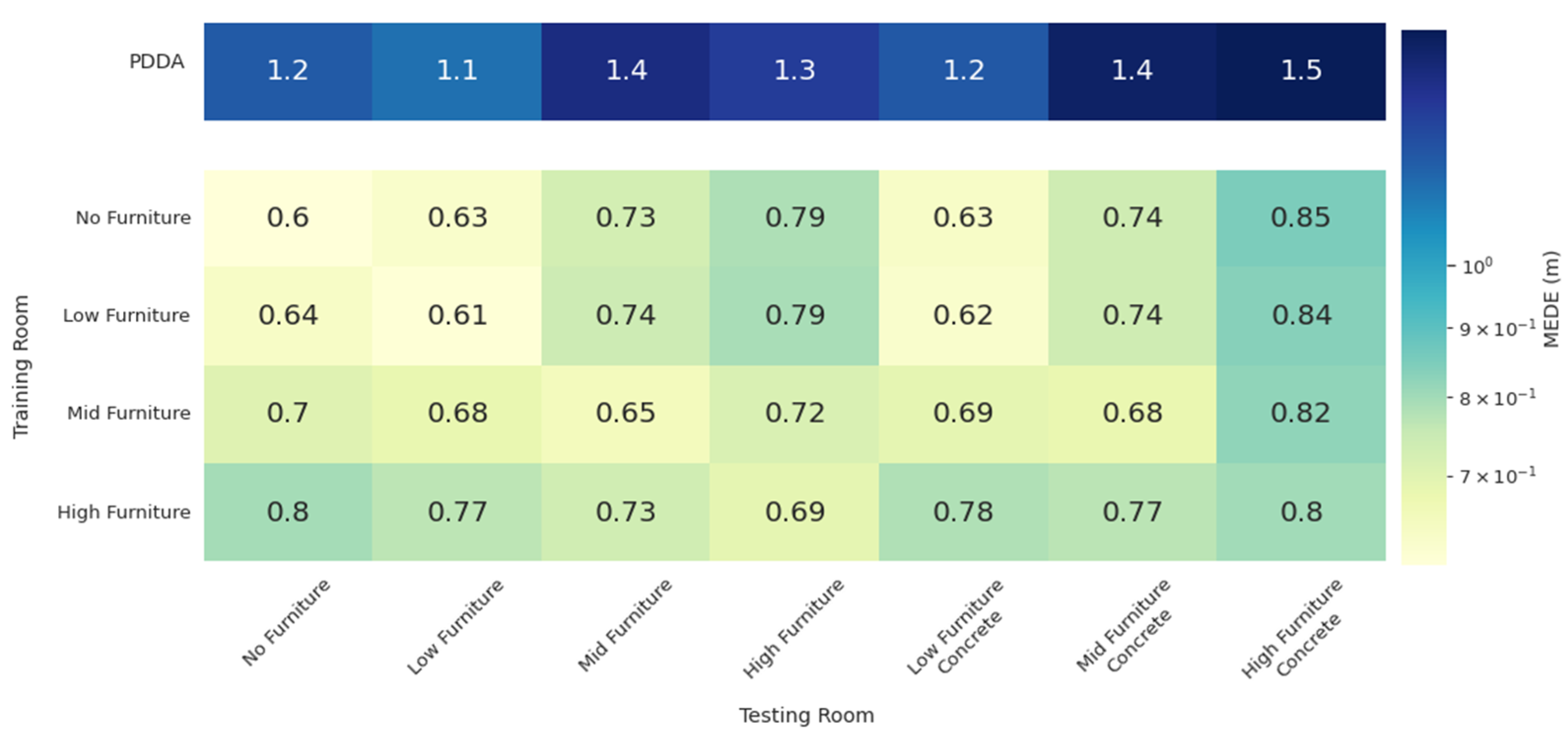
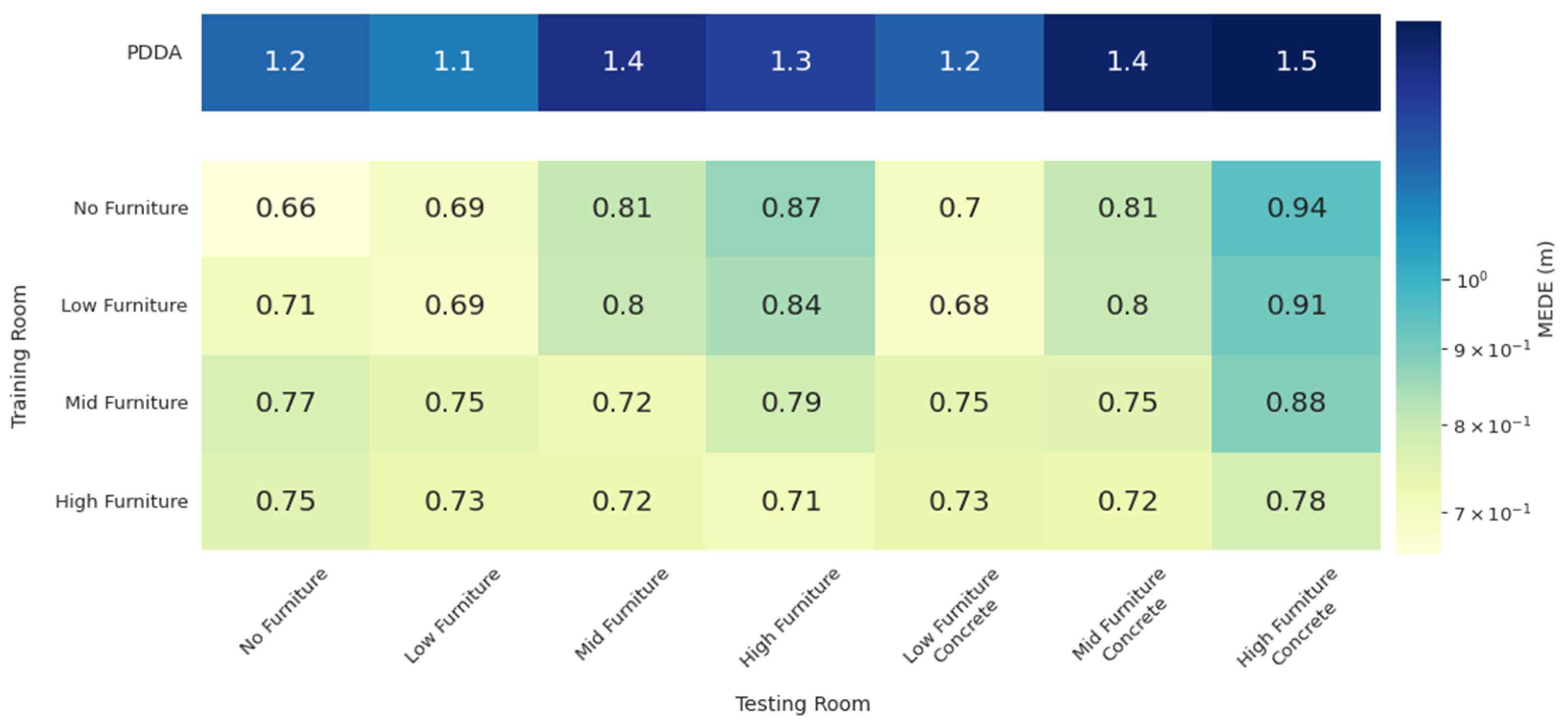
3.2. Generalization Performance on Environment Configurations Not Seen during Training
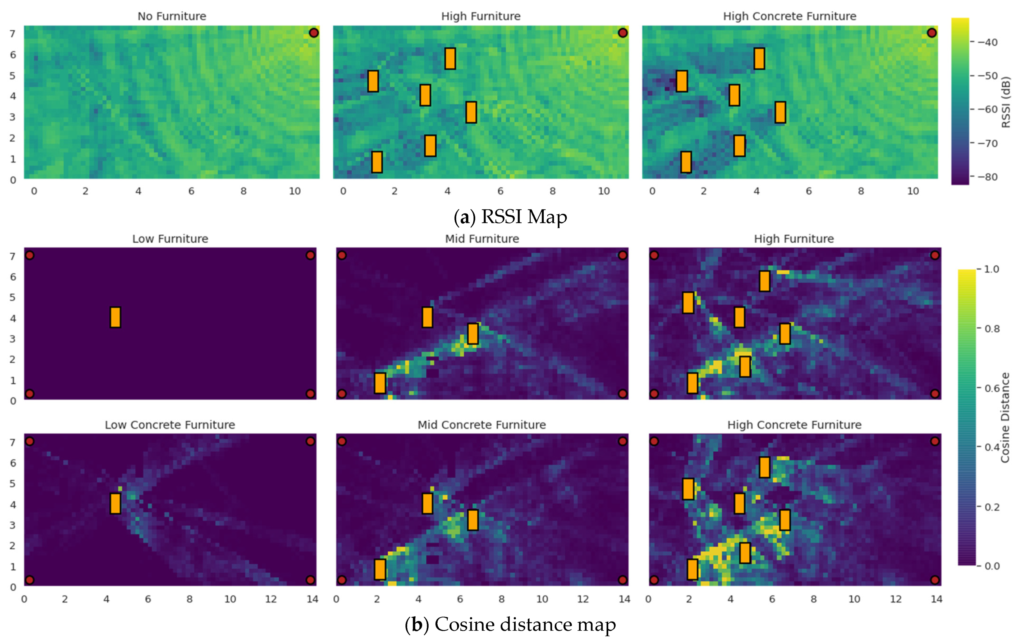
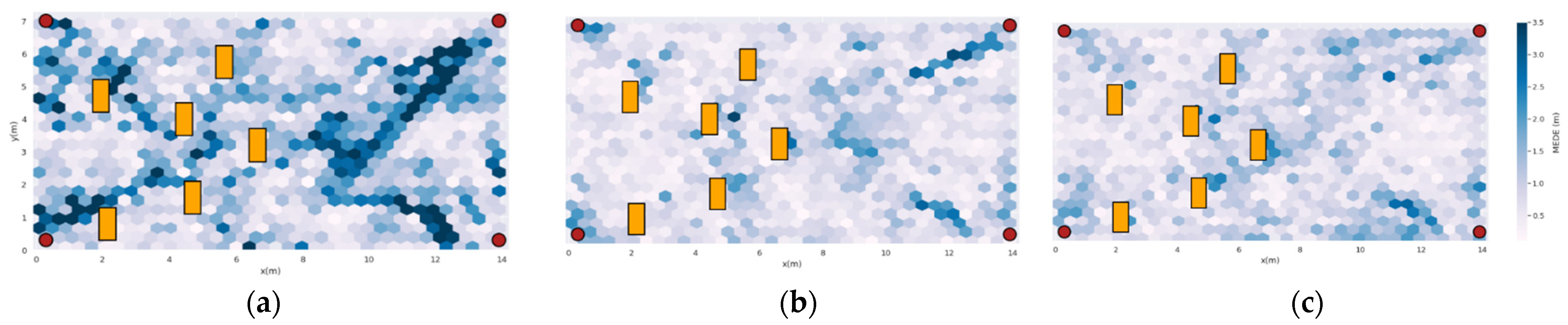
3.3. Study of the Error Spatial Distribution
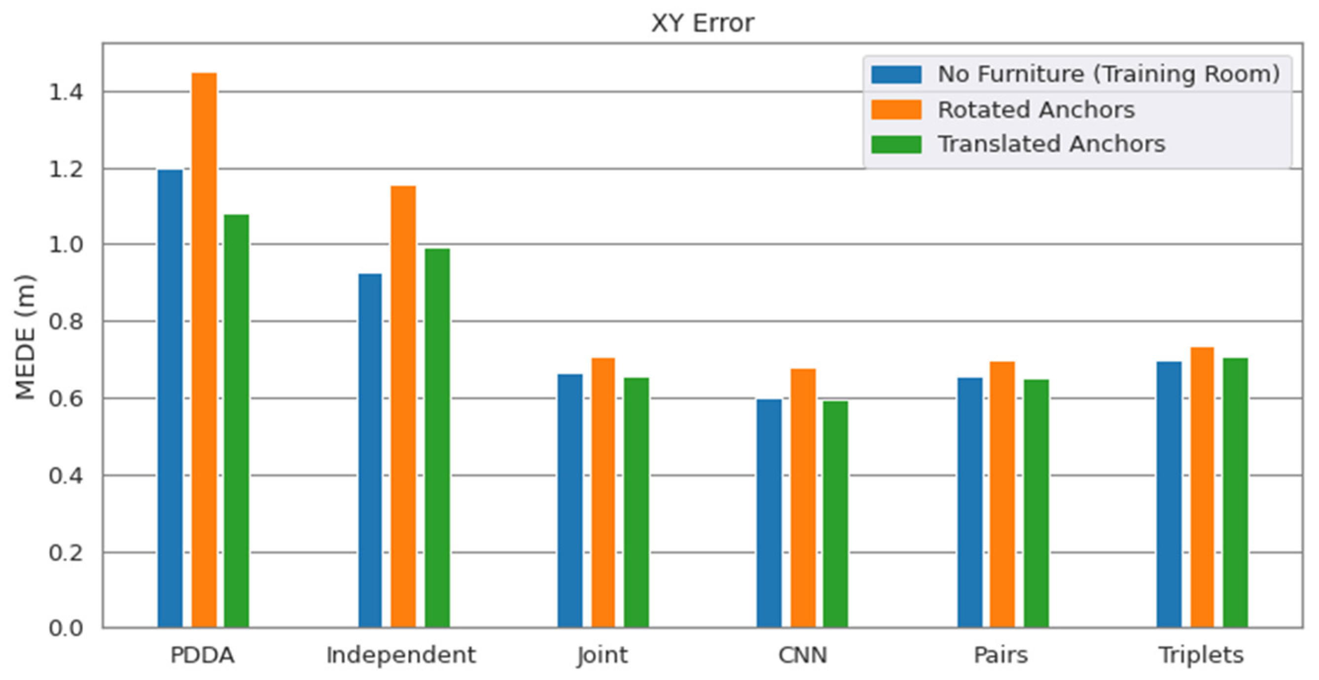
3.4. Study of Model Generalization against Moderate AP Displacements
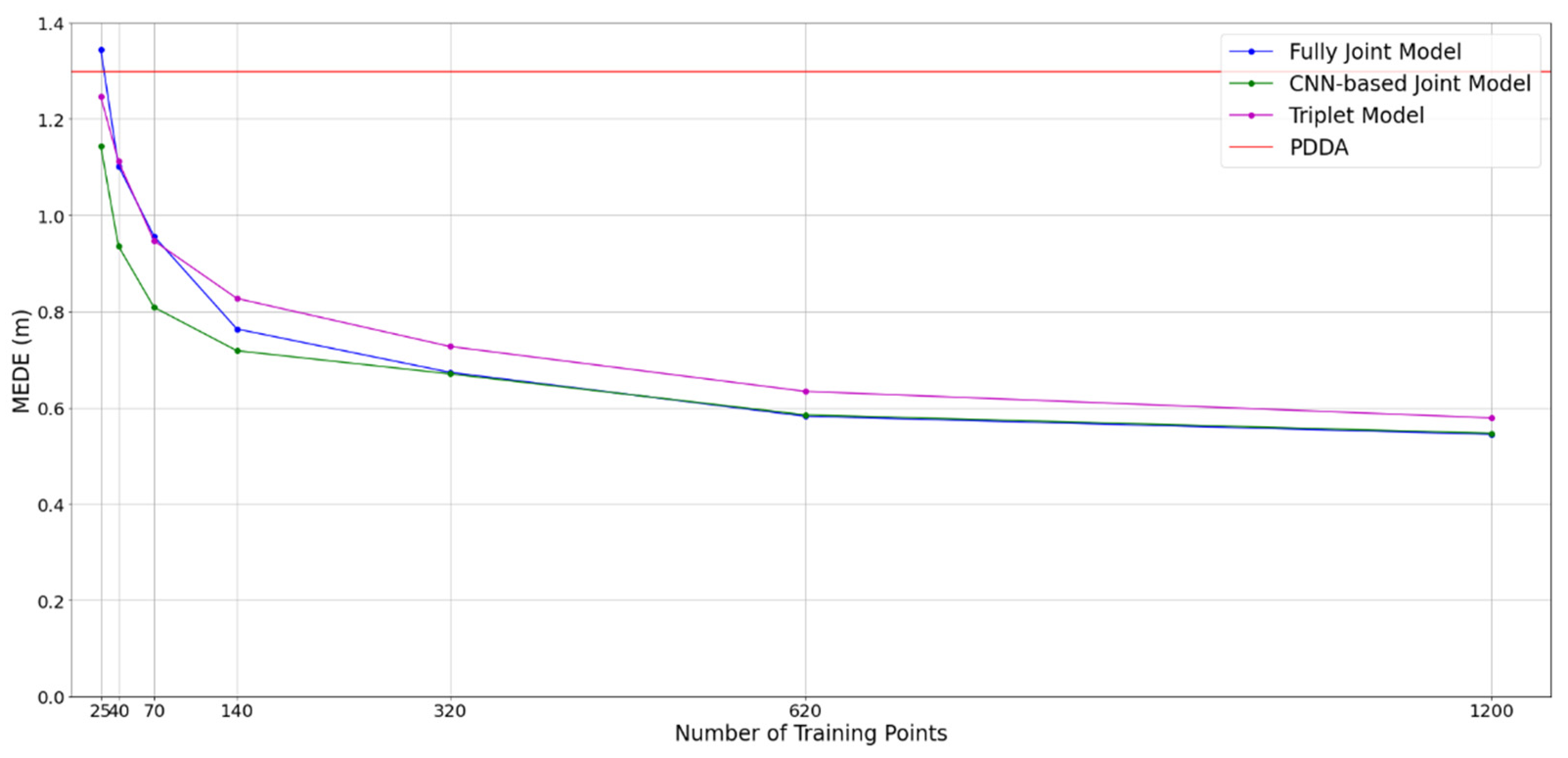
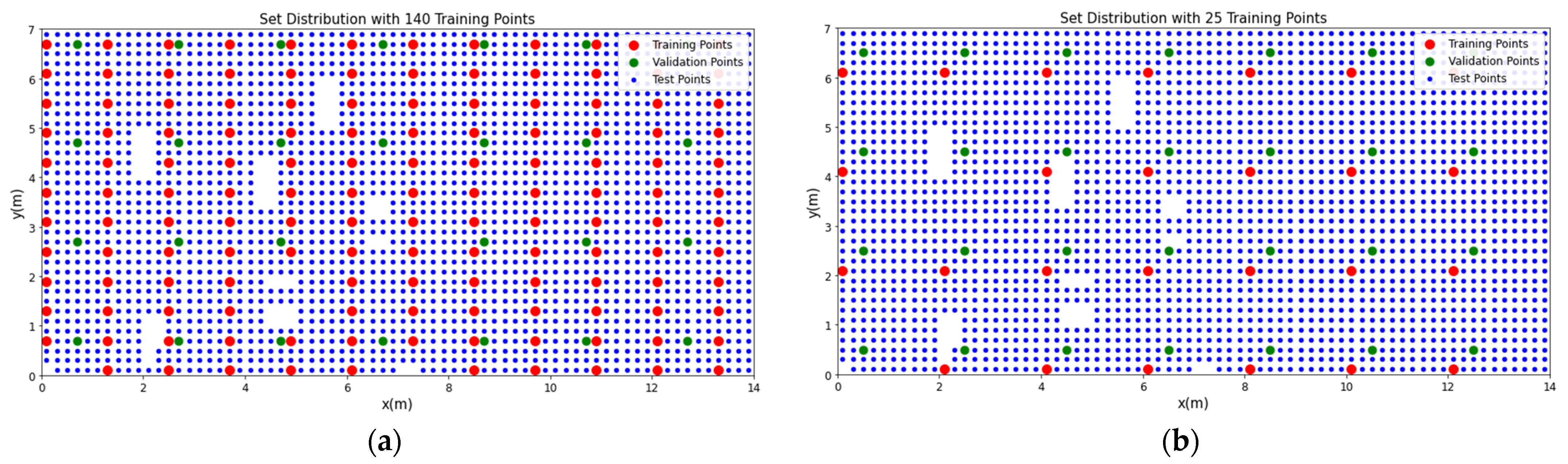
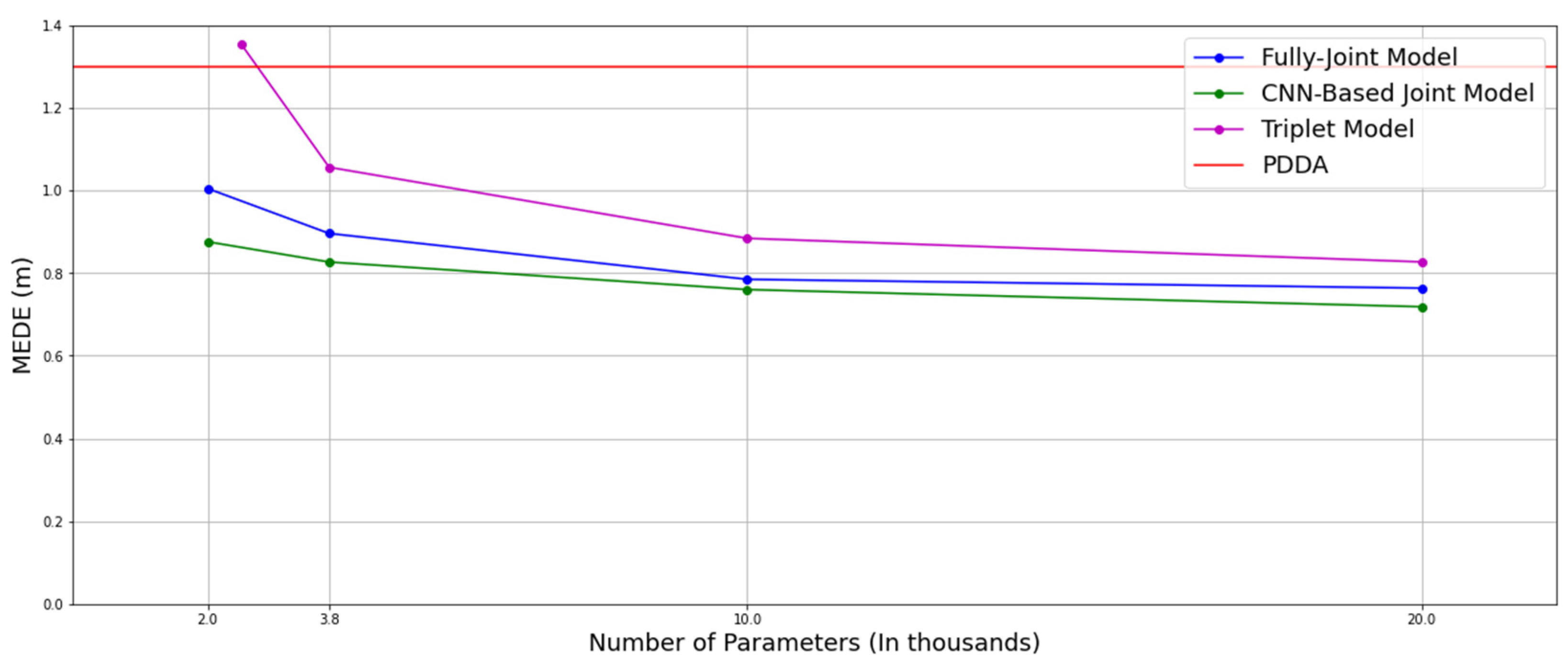
3.5. Impact of Model Size and Training Dataset Size
4. Discussion
5. Conclusions
Supplementary Materials
Author Contributions
Funding
Institutional Review Board Statement
Informed Consent Statement
Data Availability Statement
Acknowledgments
Conflicts of Interest
Abbreviations
| BLE | Bluetooth low energy |
| Τag | Transmitter |
| AP | Anchor point |
| RSSI | Received signal strength indicator |
| IQ | In-phase and quadrature-phase |
| AoA | Angle of arrival |
| ML | Machine learning |
| LS | Least squares |
| IPS | Indoor positioning system |
| UWB | Ultra-wide band |
| CTE | Constant tone extension |
| ESPRIT | Estimation of signal parameters via rotational invariance technique |
| MUSIC | Multiple signal classification |
| PDDA | Propagator direct data acquisition |
| Knn | k Nearest Neighbors |
| NN | Neural network |
| LoS | Line of sight |
| NLoS | No line of sight |
| CNN | Convolutional neural network |
| MEDE | Mean Euclidean distance error |
| MAE | Mean Absolute Error |
References
- Kim Geok, T.; Zar Aung, K.; Sandar Aung, M.; Thu Soe, M.; Abdaziz, A.; Pao Liew, C.; Hossain, F.; Tso, C.P.; Yong, W.H. Review of Indoor Positioning: Radio Wave Technology. Appl. Sci. 2021, 11, 279. [Google Scholar] [CrossRef]
- Mendoza-Silva, G.M.; Torres-Sospedra, J.; Huerta, J. A Meta-Review of Indoor Positioning Systems. Sensors 2019, 19, 4507. [Google Scholar] [CrossRef] [PubMed] [Green Version]
- Varshney, V.; Goel, R.K.; Qadeer, M.A. Indoor positioning system using Wi-Fi & Bluetooth Low Energy technology. In Proceedings of the 2016 Thirteenth International Conference on Wireless and Optical Communications Networks (WOCN), Hyderabad, India, 21–23 July 2016; pp. 1–6. [Google Scholar] [CrossRef]
- Petukhov, N.; Chugunov, A.; Zamolodchikov, V.; Tsaregorodtsev, D.; Korogodin, I. Synthesis and Experimental Accuracy Assessment of Kalman Filter Algorithm for UWB ToA Local Positioning System. In Proceedings of the 2021 3rd International Youth Conference on Radio Electronics, Electrical and Power Engineering (REEPE), Moscow, Russia, 11–13 March 2021; pp. 1–4. [Google Scholar] [CrossRef]
- Danklang, P.; Pranekunakol, T. An RSSI-based weighting with accelerometers for real-time indoor positioning. In Proceedings of the 2021 13th International Conference on Knowledge and Smart Technology (KST), Chonburi, Thailand, 21–24 January 2021; pp. 1–5. [Google Scholar] [CrossRef]
- Tekler, Z.D.; Low, R.; Gunay, B.; Andersen, R.K.; Blessing, L. A Scalable Bluetooth Low Energy Approach to Identify Occupancy Patterns and Profiles in Office Spaces. Build. Environ. 2020, 171, 106681. [Google Scholar] [CrossRef]
- Filippoupolitis, A.; Oliff, W.; Loukas, G. Occupancy Detection for Building Emergency Management Using BLE Beacons. In Computer and Information Sciences. ISCIS 2016. Communications in Computer and Information Science; Czachórski, T., Gelenbe, E., Grochla, K., Lent, R., Eds.; Springer: Cham, Switzerland, 2016; Volume 659. [Google Scholar] [CrossRef] [Green Version]
- Daniş, F.S.; Cemgil, A.T. Model-Based Localization and Tracking Using Bluetooth Low-Energy Beacons. Sensors 2017, 17, 2484. [Google Scholar] [CrossRef] [PubMed] [Green Version]
- Collotta, M.; Pau, G. A Novel Energy Management Approach for Smart Homes Using Bluetooth Low Energy. IEEE J. Sel. Areas Commun. 2015, 33, 2988–2996. [Google Scholar] [CrossRef]
- Hajiakhondi-Meybodi, Z.; Salimibeni, M.; Plataniotis, K.N.; Mohammadi, A. Bluetooth Low Energy-based Angle of Arrival Estimation via Switch Antenna Array for Indoor Localization. In Proceedings of the 2020 IEEE 23rd International Conference on Information Fusion (FUSION), Rustenburg, South Africa, 6–9 July 2020; pp. 1–6. [Google Scholar] [CrossRef]
- Gupta, P.; Verma, V.K.; Senapati, V. Angle of arrival detection by ESPRIT method. In Proceedings of the 2017 International Conference on Communication and Signal Processing (ICCSP), Chennai, India, 6–8 April 2017; pp. 1143–1147. [Google Scholar] [CrossRef]
- Schmidt, R. Multiple emitter location and signal parameter estimation. IEEE Trans. Antennas Propag. 1986, 34, 276–280. [Google Scholar] [CrossRef] [Green Version]
- Al-Sadoon, M.A.G.; Ali, N.T.; Dama, Y.; Zuid, A.; Jones, S.M.R.; Abd-Alhameed, R.A.; Noras, J.M. A New Low Complexity Angle of Arrival Algorithm for 1D and 2D Direction Estimation in MIMO Smart Antenna Systems. Sensors 2017, 17, 2631. [Google Scholar] [CrossRef] [PubMed] [Green Version]
- Ye, H.; Yang, B.; Long, Z.; Dai, C. A Method of Indoor Positioning by Signal Fitting and PDDA Algorithm using BLE AOA Device. IEEE Sens. J. 2022. [Google Scholar] [CrossRef]
- Peng, Y.; Fan, W.; Dong, X.; Zhang, X. An Iterative Weighted KNN (IW-KNN) Based Indoor Localization Method in Bluetooth Low Energy (BLE) Environment. In Proceedings of the 2016 Intl IEEE Conferences on Ubiquitous Intelligence & Computing, Advanced and Trusted Computing, Scalable Computing and Communications, Cloud and Big Data Computing, Internet of People, and Smart World Congress (UIC/ATC/ScalCom/CBDCom/IoP/SmartWorld), Toulouse, France, 18–21 July 2016; pp. 794–800. [Google Scholar] [CrossRef]
- Faragher, R.; Harle, R. Location Fingerprinting With Bluetooth Low Energy Beacons. IEEE J. Sel. Areas Commun. 2015, 33, 2418–2428. [Google Scholar] [CrossRef]
- Wang, S.; Ma, R.; Li, Y.; Wang, Q. A Bluetooth Location Method Based on kNN Algorithm. In Proceedings of the 2019 15th International Computer Engineering Conference (ICENCO), Cairo, Egypt, 29–30 December 2019; pp. 1–4. [Google Scholar] [CrossRef]
- Tasaki, K.; Takahashi, T.; Ibi, S.; Sampei, S. 3D Convolutional Neural Network-Aided Indoor Positioning Based on Fingerprints of BLE RSSI. In Proceedings of the 2020 Asia-Pacific Signal and Information Processing Association Annual Summit and Conference (APSIPA ASC), Auckland, New Zealand, 7–10 December 2020; pp. 1483–1489. [Google Scholar]
- Sun, D.; Zhang, Y.; Xia, W.; Geng, Z.; Yan, F.; Shen, L.; Gao, Y. A BLE Indoor Positioning Algorithm based on Weighted Fingerprint Feature Matching Using AOA and RSSI. In Proceedings of the 2021 13th International Conference on Wireless Communications and Signal Processing (WCSP), Changsha, China, 20–22 October 2021; pp. 1–6. [Google Scholar] [CrossRef]
- Urano, K.; Hiroi, K.; Yonezawa, T.; Kawaguchi, N. An End-to-End BLE Indoor Location Estimation Method Using LSTM. In Proceedings of the 2019 Twelfth International Conference on Mobile Computing and Ubiquitous Network (ICMU), Kathmandu, Nepal, 4–6 November 2019; pp. 1–7. [Google Scholar] [CrossRef]
- Sun, D.; Wei, E.; Ma, Z.; Wu, C.; Xu, S. Optimized CNNs to Indoor Localization through BLE Sensors Using Improved PSO. Sensors 2021, 21, 1995. [Google Scholar] [CrossRef] [PubMed]
- Kotrotsios, K.; Fanariotis, A.; Leligou, H.-C.; Orphanoudakis, T. Design Space Exploration of a Multi-Model AI-Based Indoor Localization System. Sensors 2022, 22, 570. [Google Scholar] [CrossRef] [PubMed]
- HajiAkhondi-Meybodi, Z.; Salimibeni, M.; Mohammadi, A.; Plataniotis, K.N. Bluetooth Low Energy and CNN-Based Angle of Arrival Localization in Presence of Rayleigh Fading. In Proceedings of the ICASSP 2021–2021 IEEE International Conference on Acoustics, Speech and Signal Processing (ICASSP), Toronto, ON, Canada, 6–11 June 2021; pp. 7913–7917. [Google Scholar] [CrossRef]
- Bialer, O.; Garnett, N.; Tirer, T. Performance advantages of deep neural networks for angle of arrival estimation. In Proceedings of the ICASSP 2019—2019 IEEE International Conference on Acoustics, Speech and Signal Processing (ICASSP), Brighton, UK, 12–17 May 2019. [Google Scholar]
- Khan, A.; Wang, S.; Zhu, Z. Angle-of-Arrival Estimation Using an Adaptive Machine Learning Framework. IEEE Commun. Lett. 2019, 23, 294–297. [Google Scholar] [CrossRef]
- Sayrafian-Pour, K.; Kaspar, D. Indoor positioning using spatial power spectrum. In Proceedings of the 2005 IEEE 16th International Symposium on Personal, Indoor and Mobile Radio Communications, Berlin, Germany, 11–14 September 2005; Volume 4, pp. 2722–2726. [Google Scholar] [CrossRef]
- Babakhani, P.; Merk, T.; Mahlig, M.; Sarris, I.; Kalogiros, D.; Karlsson, P. Bluetooth Direction Finding using Recurrent Neural Network. In Proceedings of the 2021 International Conference on Indoor Positioning and Indoor Navigation (IPIN), Lloret de Mar, Spain, 29 November–2 December 2021; pp. 1–7. [Google Scholar] [CrossRef]
- Merk, T.; Abou Nasa, M.; Rezai, F.; Karlsson, P.; Mahlig, M. Machine Learning calibration of Angle of Arrival methods based on different experimental Unified Linear and Rectified Array measurements. TechRxiv. Preprint. 2021. [Google Scholar] [CrossRef]
- Kim, M.; Han, D.; Rhee, J.-K.K. Multiview Variational Deep Learning With Application to Practical Indoor Localization. IEEE Internet Things J. 2021, 8, 12375–12383. [Google Scholar] [CrossRef]
- Watanabe, F. Wireless Sensor Network Localization Using AoA Measurements With Two-Step Error Variance-Weighted Least Squares. IEEE Access 2021, 9, 10820–10828. [Google Scholar] [CrossRef]

| Model | MEDE in Low Furniture (Meters) | MEDE in High Furniture (Meters) | ||
|---|---|---|---|---|
| Non-Augmented | Augmented | Non-Augmented | Augmented | |
| Independent | 1.03 ± 0.78 | 0.96 ± 0.74 | 1.10 ± 0.86 | 1.08 ± 0.86 |
| Fully Joint | 0.75 ± 0.53 | 0.65 ± 0.47 | 0.86 ± 0.60 | 0.75 ± 0.52 |
| Triplets of APs | 0.82 ± 0.52 | 0.70 ± 0.48 | 0.96 ± 0.60 | 0.84 ± 0.57 |
| Pairs of APs | 0.76 ± 0.50 | 0.69 ± 0.48 | 0.91 ± 0.57 | 0.71 ± 0.48 |
| CNN-based Joint | 0.76 ± 0.49 | 0.61 ± 0.45 | 0.87 ± 0.53 | 0.69 ± 0.50 |
| PDDA | 1.14 ± 0.95 | 1.14 ± 0.95 | 1.30 ± 1.14 | 1.30 ± 1.14 |
| Model | MAE in High Furniture (°) | |||
|---|---|---|---|---|
| AP1 | AP2 | AP3 | AP4 | |
| Independent | 5.64 ± 8.33 | 6.87 ± 7.29 | 6.27 ± 8.22 | 6.2 ± 9.37 |
| Fully Joint | 4.18 ± 7.80 | 4.44 ± 5.51 | 3.89 ± 4.79 | 4.38 ± 7.06 |
| Triplets of APs | 4.54 ± 6.96 | 4.62 ± 6.29 | 4.26 ± 5.34 | 4.82 ± 6.92 |
| Pairs of APs | 4.02 ± 7.35 | 4.25 ± 5.48 | 3.99 ± 5.15 | 4.03 ± 6.50 |
| CNN-based Joint | 4.03 ± 6.76 | 3.89 ± 4.86 | 3.50 ± 4.8 | 4.31 ± 6.98 |
| PDDA | 5.80 ± 9.14 | 8.38 ± 10.34 | 5.86 ± 9.57 | 7.40 ± 11.26 |
| Model | MEDE (m) | |
|---|---|---|
| Left Half (Furniture Dense) | Right Half (Furniture Free) | |
| Independent | 1.12 | 1.13 |
| Fully Joint | 0.80 | 0.79 |
| Triplets of APs | 0.79 | 0.88 |
| Pairs of APs | 0.80 | 0.88 |
| CNN-based Joint | 0.73 | 0.85 |
| PDDA | 1.23 | 1.36 |
| Model | Description | Advantages | Disadvantages |
|---|---|---|---|
| Independent | AoA computed independently by each AP | Simple implementation, Distributed computation | Lower accuracy compared to the rest of the models |
| Fully Joint | Joint estimation of all AoAs by a single ML model | High accuracy | All raw data need to be transferred to a central unit for computation |
| Tuples of APs | Joint estimation of AoAs by forming groups of APs | High accuracy, Distributed computation | Performance degrades faster compared to the rest of the models when lower complexity NN configurations are adopted. |
| CNN-based Joint | Joint estimation of AoAs by a single CNN | Highest accuracy, Most robust approach to complexity reduction and to smaller training size | All raw data need to be transferred to a central unit for computation |
Publisher’s Note: MDPI stays neutral with regard to jurisdictional claims in published maps and institutional affiliations. |
© 2022 by the authors. Licensee MDPI, Basel, Switzerland. This article is an open access article distributed under the terms and conditions of the Creative Commons Attribution (CC BY) license (https://creativecommons.org/licenses/by/4.0/).
Share and Cite
Koutris, A.; Siozos, T.; Kopsinis, Y.; Pikrakis, A.; Merk, T.; Mahlig, M.; Papaharalabos, S.; Karlsson, P. Deep Learning-Based Indoor Localization Using Multi-View BLE Signal. Sensors 2022, 22, 2759. https://doi.org/10.3390/s22072759
Koutris A, Siozos T, Kopsinis Y, Pikrakis A, Merk T, Mahlig M, Papaharalabos S, Karlsson P. Deep Learning-Based Indoor Localization Using Multi-View BLE Signal. Sensors. 2022; 22(7):2759. https://doi.org/10.3390/s22072759
Chicago/Turabian StyleKoutris, Aristotelis, Theodoros Siozos, Yannis Kopsinis, Aggelos Pikrakis, Timon Merk, Matthias Mahlig, Stylianos Papaharalabos, and Peter Karlsson. 2022. "Deep Learning-Based Indoor Localization Using Multi-View BLE Signal" Sensors 22, no. 7: 2759. https://doi.org/10.3390/s22072759
APA StyleKoutris, A., Siozos, T., Kopsinis, Y., Pikrakis, A., Merk, T., Mahlig, M., Papaharalabos, S., & Karlsson, P. (2022). Deep Learning-Based Indoor Localization Using Multi-View BLE Signal. Sensors, 22(7), 2759. https://doi.org/10.3390/s22072759